A Second Order Weighted Numerical Scheme on Nonuniform Meshes for Convection Diffusion Parabolic Problems

Lolugu Govindarao and Jugal Mohapatra*

Department of Mathematics, National Institute of Technology Rourkela – 769008, India

E-mail: jugal@nitrkl.ac.in

* Corresponding Author

Received 09 February 2019; Accepted 03 December 2019; Publication 14 January 2020

Abstract

In this article, a singularly perturbed parabolic convection-diffusion equation on a rectangular domain is considered. The solution of the problem possesses regular boundary layer which appears in the spatial variable. To discretize the time derivative, we use two type of schemes, first the implicit Euler scheme and second the implicit trapezoidal scheme on a uniform mesh. For approximating the spatial derivatives, we use the monotone hybrid scheme, which is a combination of midpoint upwind scheme and central difference scheme with variable weights on Shishkin-type meshes (standard Shishkin mesh, Bakhvalov-Shishkin mesh and modified Bakhvalov-Shishkin mesh). We prove that both numerical schemes converge uniformly with respect to the perturbation parameter and are of second order accurate. Thomas algorithm is used to solve the tri-diagonal system. Finally, to support the theoretical results, we present a numerical experiment by using the proposed methods.

Keywords: Singular perturbation, parabolic problems, boundary layer, monotone/weighted schemes, uniform convergence, implicit schemes.

1 Introduction

The theory of singular perturbation is a developing mathematical subject with a long history and a strong promise for continued important applications throughout science and engineering. We can find singular perturbation problems in a lot of areas of Engineering, Biological science and Applied Mathematics, e.g., Fluid mechanics, Quantum mechanics, Elasticity, Chemical reactor theory, Magneto hydrodynamics and Reaction diffusion process, etc. With immense growth of science and technology day by day, many practical problems in boundary layer theory or approximation of solution of various problems can be described by ordinary or partial differential equations. When very small parameters are involved, problems are typically termed perturbed problems. These problems are become more and more difficult to solve and we require the use of asymptotic approach. However, the theory of asymptotic analysis for differential operators has mainly been developed for regular perturbations where the perturbations are subordinate to the unperturbed operator. In some problems, the perturbations are operative over very narrow regions across which the dependent variable undergoes very rapid changes. These narrow regions known as boundary layers, frequently adjoin the boundaries of the domain of interest. Owing to the fact that the small parameter multiplies the highest derivative making the problem singularly perturbed problem (SPP). Consequently, these narrow regions referred as boundary layers in fluid mechanics, edge layers in solid mechanics, skin layers in electrical applications, transition points in quantum mechanics and Stokes lines and surfaces in Mathematics (refer ‘(Bansal et al., 2017; Shishkin & Shishkina, 2009)’ and references therein). It is known that SPPs are difficult to solve by using the standard numerical methods on uniform meshes. Due to the presence of the small parameter (ε) in these initial-boundary-value problems, standard numerical methods on uniform mesh fail to give accurate results and usually are unstable when ε tends to zero. Thus to achieve accurate numerical solution, we need large number of mesh points where the mesh size matches with the order of ε which is unacceptable due to the massive computational cost. This drawback motivates to develop ε-uniform numerical methods (refer Brandt & Yavneh (1991); Kellogg & Tsan (1978)). At the same time, we have several results which deals with the numerical solution of parabolic SPP. To cite a few on Shishkin-type meshes, graded meshes and adaptive meshes, one can refer Clavero et al. (2005); Linß et al. (2000) where the authors proposed ε-uniformly convergent finite difference schemes. Also for p-refinement, XFEM, one may refer Gartland (1988a), O’Riordan & Stynes (1991) and Guo & Stynes (1993).

The robust approximation of boundary layers requires either the use of the h version on non-uniform meshes, or the use of the high order p and hp versions on specially designed meshes Schwab et al. (1996). In both cases, the a-priori knowledge of the position of the layers is taken into account. One dimensional SPP numerically solved in Schwab et al. (1996) by using h, p, hp-refinement meshes and they have shown that solutions are more accurate on hp-refinement mesh comparing with h and p-refinement. A coupled system of singularly perturbed reaction-diffusion equations approximated by the hp-FEM in Melenk et al. (2013). Singularly perturbed boundary value problems on smooth domains and non-smooth domains solved in Xenophontos (1998a) by using h − p finite element method.

A typical transport mechanism involving time-dependent convection-diffusion, with convection being the dominant process, can be expressed as $\varphi \frac{\partial u}{\partial t}-\nabla \cdot (D\nabla u)+v\cdot \nabla u=F$. This equation is mostly used in soil science, chemical, environmental, and petroleum reservoir engineering, and water resources. Some of the known applications include the movement of ammonium or nitrate in soils ‘(Misra & Mishra, 1977)’, pesticide movement ‘(Kay & Elrick, 1967)’, the transport of radioactive waste materials. To clearly understand the phenomena of moving sharp fronts of this equation and the techniques of singular perturbation, we consider the following singularly perturbed parabolic convection-diffusion initial-boundary-value problem (IBVP) with Dirichlet boundary conditions:

$$\{\begin{array}{l}\left(\frac{\partial }{\partial t}+L_{\epsilon ,x}\right)u(x,t)=f(x,t),(x,t)\in D,\hfill \\ u(x,0)=u_0(x),u(0,t)=u(1,t)=0,t\in (0,T],x\in [0,1],\hfill \end{array}$$

(1)

where D = (0,1) × (0,T]. The operator L_ε,x is defined as: L_ε,xu(x, t) = −εu_xx(x, t) − a(x)u_x(x, t) + b(x)u(x, t), 0 < ε ≪ 1 and the coefficients a(x), b(x) are sufficiently smooth functions such that a(x) ≥ α > 0, b(x) ≥ β ≥ 0 on D. Under sufficiently smoothness and compatibility conditions on the functions u₀ and f, the IBVP (1), in general admits a unique solution u(x, t). The exact solution of (1) has a regular layer of order 𝒪(ε) located at the boundary x = 0 of D.

There are research articles which deal with various numerical methods for convection-diffusion problems. In last few decades, many researchers have developed ε-uniform numerical methods for stationary and non stationary problems; for more information, one can refer to the recent books ‘(Miller et al., 2012; Shishkin & Shishkina, 2009)’. To refer few articles; Clavero et al. in ‘(Clavero et al., 2003)’ solved the parabolic convection-diffusion equation by using the upwind scheme on a special nonuniform mesh for the spatial discretization and they shown the order of convergence is almost one. Stynes and O’Riordan in ‘(Ng-Stynes et al., 1988)’ solved the time dependent convection-diffusion equations, Stynes and Roos in (Stynes & Roos, 1997) used the midpoint upwind scheme to solve the time independent convection-diffusion problem by using the hybrid method, Mukherjee and Natesan in ‘(Mukherjee & Natesan, 2009)’ solved the time dependent convection-diffusion problem. They shown the rate of convergence is almost first order in time direction and almost second order up to a logarithm factor in spatial direction. In order to show globally the second order rate of convergence both with respect to time and space, they assumed square of number of mesh points in spatial variable equal to number of mesh points in temporal direction. Andreev and Kopteva solved the convection-diffusion problem in ‘(Andreev & Kopteva, 1998)’ using the monotone three-point finite difference scheme and shown the second order rate of convergence on a Bakhvalov mesh and the second order rate of convergence upto logarithm factor on a Shishkin mesh. Linß ‘(Linß, 2001)’ provided the sufficient condition for uniform convergence on layer-adapted grids for quasilinear convection-diffusion problems.

Here, in this work, we have solved the IBVP(1) by using the implicit Euler for descretization in time and a monotone hybrid scheme to discretize in space, which is a combination of the midpoint and the central difference scheme with variable weights on the Shishkin-type-meshes to get the optimal order of convergence. The hybrid scheme discussed in ‘(Stynes & Roos, 1997)’ is a combination of the the midpoint and the central difference scheme, where a apriori information is needed to switch from the midpoint scheme to the central difference scheme as the mesh goes from coarse to fine. But in the weighted monotone hybrid scheme discussed here, the weights are so chosen that the scheme is automatically switched from midpoint scheme to central difference scheme as the mesh goes from coarse to fine and so, having the advantage for over the hybrid scheme discussed in ‘(Stynes & Roos, 1997)’. Again, to obtain the second order accuracy with respect to time, we use the implicit trapezoidal for time discretization. The main aim in this work is to obtain a second order accuracy both with respect to time and space without the restriction mentioned earlier in ‘(Mukherjee & Natesan, 2009)’. Again for computational purpose, we use the Thomas algorithm which is more efficient and reduce the time over the usual matrix inverse method used in the earlier articles mentioned above.

This paper is organized as follows. In Section 2, we study the bounds of the solution and its derivatives. In Section 3, we describe the Shishkin-type meshes (Shishkin mesh (S-mesh), Bakhvalov-Shishkin mesh (B-S mesh) and modified Bakhvalov-Shishkin mesh (M-B-S mesh)) and the construction of the finite difference schemes. Section 4 is devoted to the study of the uniform convergence of the finite difference schemes. Numerical results are discussed in Section 5 in shapes of tables and figures.

Throughout this paper, ‘C’ denotes a generic positive constant independent of ε, the mesh points and the mesh size. The subscripted C’s are fixed constants. Here, ‖.‖ denotes the standard supremum norm, which is defined as ‖f‖_∞ = sup_(x,t)∈D |f(x, t)|, for a function f defined on some domain D.

2 Analytic Behavior of the Solution

The operator $\left(\frac{\partial }{\partial t}+L_{\epsilon ,x}\right)$ in (1) satisfies the following maximum principle:

Lemma 2.1. (Maximum principle) Suppose the function $\psi (x,t)\in C^0(\overline{D})\cap C^2(D)$, satisfies $\left(\frac{\partial }{\partial t}+L_{\epsilon ,x}\right)\psi (x,t)\ge 0$ in D, ψ(x, t) ≥ 0 on Γ. Then ψ(x, t) ≥ 0 for all $(x,t)\in \overline{D}=[0,1]\times (0,T]$.

Proof. Let $\mathrm{<mo\; stretchy="false">(</mo>}{x}^{\mathrm{<mo>*</mo>}}\mathrm{,}{t}^{\mathrm{<mo>*</mo>}}\mathrm{<mo\; stretchy="false">)</mo>}\in \overline{D}$ such that $\psi (x^{*},t^{*})={{\displaystyle \min }}_{(x,t)\in \overline{D}}\psi (x,t)$ and assume that ψ(x*, t*) < 0. Clearly, (x*, t*) ∉ Γ for (x*, t*) ∈ D. As it attains minimum at (x*, t*), we have ψ_x = 0, ψ_t = 0 and ψ_xx ≥ 0 at (x*, t*). Therefore, from (1), we have $\left(\frac{\partial }{\partial t}+L_{\epsilon ,x}\right)\psi (x^{*},t^{*})<0$, which is a contradiction as $\left(\frac{\partial }{\partial t}+L_{\epsilon ,x}\right)\psi (x,t)\ge 0$. Hence, $\psi (x,t)\ge 0\forall \mathrm{<mi>\; </mi>}(x,t)\in \overline{D}$. One can refer the book for more details ‘(Farrell et al., 2000)’.

It is known that if $u_0\in C^0(\overline{\Gamma })$, $f\in C^0(\overline{D})$ and u₀(0) = u₀(1) = 0, then $u\in C^0(\overline{D})$. The maximum principle together with ε-uniform bounds for f and u₀ give the uniform bound |u(x, t)| ≤ C for all $(x,t)\in \overline{D}$.

Lemma 2.2. The solution u(x, t) of (1) satisfies $\left|\frac{{\partial }^{i}u(x,t)}{\partial t^i}\right|\le C$, $\left(x,t\right)\in \overline{D}$, i = 1,2, 3.

Proof. First we prove for i = 1. We have u ≡ 0 on the sides x = 0 and x = 1 on $\overline{D}$, and so u_t ≡ 0. From (1), we have u(x, 0) = u₀(x) and also we know |u(x, t)| ≤ C. So for the side t = 0, we can choose C₁ sufficiently large such that |u_t| ≤ C₁ on three sides of $\overline{D}$. Consider the operator ‘L’ defined by $\mathit{Lu}=\left(\frac{\partial }{\partial t}+L_{\epsilon ,x}\right)u$, then L satisfies the maximum principle on $\overline{D}$. Now L(u_t)(x, t) = f_t so |Lu_t(x, t)| ≤ C₂. Following the idea of the proof given in Lemma 4.4 of ‘(Ng-Stynes et al., 1988)’, one can get $\left|\frac{\partial u(x,t)}{\partial t}\right|\le \mathrm{<mi>\; </mi>}C,(x,t)\in \overline{D}$. Similarly differentiating further, we can also prove for i = 2, 3. Hence, $\left|\frac{{\partial }^{i}u(x,t)}{\partial t^i}\right|\le C,(x,t)\in \overline{D}$.

2.1 Decomposition of the Solution

To obtain the ε uniform error estimate, we need more intrinsic bounds on the derivatives of the solution u(x, t) of (1). We decompose u as u = v + w, where v and w are the regular and the singular component respectively. We express the regular component v as $v(x,t)={\displaystyle {\sum }_{k=0}^4}{\epsilon }^k{v}_k(x,t)$, (x, t) ∈ D, where v_k(x, t), for k = 0, 1, 2, 3, are the solutions of the following first order PDEs (12)-(3)

$$\{\begin{array}{l}{(v_0)}_t(x,t)-a(x){(v_0)}_x(x,t)+b(x,t)(v_0)(x,t)=f(x,t),(x,t)\in D\hfill \\ (v_0)(x,t)=u(x,0),x\in (0,1),(v_0)(0,t)=0,t\in [0,T],\hfill \end{array}$$

(2)

and

$$\{\begin{array}{l}{(v_k)}_t(x,t)-a(x){(v_k)}_x(x,t)+b(x,t)(v_k)(x,t)=\frac{{\partial }^2{v}_{k-1}}{\partial x^2},(x,t)\in D\hfill \\ (v_k)(x,0)=0,x\in (0,1),k=1,2,3,\hfill \\ (v_k)(0,t)=0,t\in [0,T],\hfill \end{array}$$

(3)

the final component v₄ satisfies

$$\{\begin{array}{l}\left(\frac{\partial }{\partial t}+L_{\epsilon ,x}\right)v_4(x,t)=\frac{{\partial }^2{v}_3}{\partial x^2},(x,t)\in D\hfill \\ (v_4)(x,0)=0,x\in (0,1),(v_4)(0,t)=(v_4)(1,t)=0,t\in [0,T].\hfill \end{array}$$

(4)

The regular component v(x, t) satisfies the following problem:

$$\{\begin{array}{l}\left(\frac{\partial }{\partial t}+L_{\epsilon ,x}\right)v(x,t)=f(x,t),(x,t)\in D\hfill \\ v(x,0)=u(x,0),x\in (0,1),\hfill \\ v(0,t)={\displaystyle \sum _{k=0}^4}{\epsilon }^k{v}_k(0,t),v(1,t)=0,t\in [0,T],\hfill \end{array}$$

(5)

and the singular component w(x, t) satisfies the PDE

$$\{\begin{array}{l}\left(\frac{\partial }{\partial t}+L_{\epsilon ,x}\right)w(x,t)=0,(x,t)\in D\hfill \\ w(x,0)=0,x\in (0,1),\hfill \\ w(0,t)=u(0,t)-v(0,t),w(1,t)=0,t\in [0,T].\hfill \end{array}$$

(6)

The following theorem provides the bounds for the derivatives of the regular component and the singular component respectively.

Theorem 2.3. The solution u(x, t) of the problem (1) admits the decomposition u(x, t) = v(x, t) + w(x, t), then for all non-negative integers l, m, satisfying 0 ≤ l + m ≤ 5, the regular component v(x, t) satisfies

$$\left|\frac{{\partial }^{l+m}v}{\partial x^l\partial t^m}\right|\le C+({\epsilon }^{4-l}),$$

and the singular component w(x, t) satisfies

$$\left|\frac{{\partial }^{l+m}w}{\partial x^l\partial t^m}\right|\le C{\epsilon }^{-l}({\epsilon }^2+\exp (-\alpha x/\epsilon )),(x,t)\in D.$$

One may refer ‘(Farrell et al., 2000)’ for the proof.

3 Finite Difference Method

3.1 The Semidiscretization

For the time domain [0, T], we use the uniform time step Δt and the discretization is

$$G_t^M=\{t_n=n\Delta t,n=0\dots M,\mathrm{<mi>\; </mi>}{t}_M=T,\Delta t=T/M\},$$

where M is number of mesh subintervals for t-direction in [0, T]. To discretize (1), first we use the implicit Euler method defined as:

$$\{\begin{array}{l}{u}^{0,1}=u_0(x),\hfill \\ (I+\Delta t{L}_{\epsilon ,x})u^{n+1,1}=u^{n,1}+\Delta t{f}^{n+1},\hfill \\ u^{n+1,1}(0)=u^{n+1,1}(1)=0,\hfill \end{array}$$

(7)

and then we use the implicit trapezoidal method defined as:

$$\{\begin{array}{l}{u}^{0,2}=u_0(x),\hfill \\ \left(I+\frac{\Delta t}{2}{L}_{\epsilon ,x}\right)u^{n+1,2}=\frac{\Delta t}{2}(f^{n+1}+f^n)+\left(I-\frac{\Delta t}{2}{L}_{\epsilon ,x}\right)u^{n,2},\hfill \\ u^{n+1,2}(0)=u^{n+1,2}(1)=0.\hfill \end{array}$$

(8)

Here, I is the identity operator, fⁿ = f(x, t_n), u^n,j = u(x, t_n) for j = 1, 2 is the semidiscrete approximation to the exact solution u(x, t) of (1) at the time level t_n = nΔt. We write (7) and (8) in the following form:

$$\begin{array}{lll}\hfill u^{0,j}& \hfill =\hfill & u_0(x),\hfill \\ \hfill T{u}^{n+1,j}(x)& \hfill =\hfill & F^n(x),\hfill \\ \hfill u^{n+1,j}(0)& \hfill =\hfill & u^{n+1,j}(1)=0,0\le x\le 1,\text{for }j=1,2,\hfill \end{array}$$

where

$$T{u}^{n+1,j}(x)=-\epsilon u_{xx}^{n+1,j}(x)-a(x)u_x^{n+1,j}(x)+d(x)u^{n+1,j}(x),\text{for }j=1,2.$$ $$F^n(x)=\{\begin{array}{l}\frac{u^{n,1}(x)}{\Delta t}+f^{n+1}(x),\mathrm{for\; the\; implicit\; Euler\; method},\hfill \\ f^{n+1}(x)+f^n(x)+\frac{2u^{n,2}(x)}{\Delta t}-L_{\epsilon ,x}{u}^{n,2}(x),\hfill \\ \mathrm{for\; the\; implicit\; trapizodal\; method}.\hfill \end{array}$$

Here,

$d(x)=\{\begin{array}{l}b(x)+\frac{1}{\Delta t},\mathrm{for\; the\; implicit\; Euler\; method},\hfill \\ b(x)+\frac{2}{\Delta t},\mathrm{for\; the\; implicit\; trapizodal\; method}.\hfill \end{array}$

The local error is defined by $\Vert e_{j,n+1}\Vert =\left|u(x,t_{n+1})-{\widehat{u}}^{n+1,j}\right|$ for j = 1, 2, where ${\hat{u}}^{n+1,j}$ is solution obtained after one step of the semidiscrete scheme taking the exact value u(x, t_n), instead of u^n,1 as the starting data. Concretely, we have the implicit Euler method, given by

$$\{\begin{array}{l}(I+\Delta t{L}_{\epsilon ,x}){\widehat{u}}^{n+1,1}=u(x,t_n)+\Delta t{f}^{n+1},\hfill \\ {\hat{u}}^{n+1,1}(0)={\hat{u}}^{n+1,1}(1)=0,\hfill \end{array}$$

and then the implicit trapezoidal method as:

$$\{\begin{array}{l}\left(I+\frac{\Delta t}{2}{L}_{\epsilon ,x}\right){\hat{u}}^{n+1,2}=\frac{\Delta t}{2}(f^{n+1}+f^n)+\left(I-\frac{\Delta t}{2}{L}_{\epsilon ,x}\right)u(x,t_n),\hfill \\ {\hat{u}}^{n+1,2}(0)={\hat{u}}^{n+1,2}(1)=0.\hfill \end{array}$$

(9)

To obtain the convergence of the solution u^n,1 of the implicit Euler method (7), we study the consistency and the stability in the maximum norm. The stability of (7) follows from the maximum principle for the operator I+ ΔtL_x,ε, as ${\Vert {(I+\Delta t{L}_{x,\epsilon })}^{-1}\Vert }_{\infty }\le \frac{1}{1+\beta \Delta t}$. The consistency of the solution (7) follows from the following lemma.

Lemma 3.1. If $\left|\frac{{\partial }^i}{\partial t^i}u(x,t)\right|\le C$, for $(x,t)\in \overline{D}=[0,1]\times [0,T]$, for 0 ≤ i ≤ 2, the local error associated with scheme (7) satisfies ‖e_1,n+1‖ ≤ C (Δt)².

The proof of this lemma can be found in ‘(Clavero et al., 2003)’.

Now in order to obtain the first order convergence of the scheme (7), we need to combine the consistency and the stability results.

Theorem 3.2. Under the hypothesis of Lemma 3.1, the global error estimate E_n in the time direction at n^th level is bounded by ‖E_1,n‖_∞ ≤ CΔt, ∀n ≤ T/Δt.

Using the local error estimate up to n^th time step given in Lemma 3.1, we get the global error estimate at (n + 1)^th time step, One can find the detailed proof this theorem in ‘(Clavero et al., 2003)’.

We follow the idea given in ‘(Clavero et al., 2005; Kumar & Sekhara Rao, 2010)’, to obtain the convergence of the solution u^n,2 of the implicit trapezoidal scheme (8).

Lemma 3.3. If $\left|\frac{{\partial }^i}{\partial t^i}u(x,t)\right|\le C$, $\forall (x,t)\in \overline{D}$, for 0 ≤ i ≤ 3, the local error associated with the scheme (8) satisfies

$$\Vert e_{2,n+1}\Vert \le C{(\Delta t)}^3.$$

(10)

Proof. Using the central difference formula, we have

$$\begin{array}{l}\frac{u(x,t_{n+1})-u(x,t_n)}{\Delta t}=u_t(x,t_{n+\Delta t/2})+𝒪(\Delta t^2),\hfill \\ =-L_{\epsilon ,x}u(x,t_{n+\Delta t/2})+f(x,t_{n+\Delta t/2})+𝒪(\Delta t^2).\hfill \end{array}$$

Again, we know that $f(x,t_{n+\Delta t/2})=\frac{f^{n+1}+f^n}{2}+𝒪(\Delta t^2)$, so we can write

$$L_{\epsilon ,x}u(x,t_{n+\Delta t/2})=L_{\epsilon ,x}\frac{u(x,t_{n+1})+u(x,t_n)}{2}+𝒪(\Delta t^2).$$

It is straight forward to show that the local error ‖e_2,n+1‖ is the solution of the following BVP:

$$\{\begin{array}{l}\left(I+\frac{\Delta t}{2}{L}_{\epsilon ,x}\right)e_{2,n+1}=𝒪(\Delta t^3),\hfill \\ e_{2,n+1}(0)=0,e_{2,n+1}(1)=0.\hfill \end{array}$$

Then, using the maximum principle for the operator $\left(I+\frac{\Delta t}{2}{L}_{\epsilon ,x}\right)$ proves the desired result. One can refer ‘(Clavero et al., 2005)’ for the details of the argument.

Let E_2,n+1 = |u(x, t_n+1) − u^n+1,2(x)| be the global error associated with the scheme (8). Then it can be written as E_2,n+1 = e_n+1 + RE_2,n, where

$$R={\left(I+\frac{\Delta t}{2}{L}_{\epsilon ,x}\right)}^{-1}\left(I-\frac{\Delta t}{2}{L}_{\epsilon ,x}\right)$$

is the transition operator defined as follows: RE_2,n is the result obtained after one time step of (8) using uⁿ = E_2,n as the starting data, null boundary condition and zero source term f. Using this we get the recurrence relation $E_{2,n+1}={\displaystyle {\sum }_{k=0}^n}{R}^{n-k}{e}_{2,k+1}$ Thus, if the power of the transition operator R preserves the uniform bounded ness behaviour, that is,

$${\Vert R^j\Vert }_{\infty }\le C\forall j=0,1,\dots ,n,$$

(11)

then it immediately follows that sup_nΔt≤T ‖E_2,n+1‖_∞ ≤ C(Δt)², i.e, the semidiscrete scheme (8) is parameter uniformly convergent and is second order accurate. Note that (11) is typically a stability condition. The stability condition (11) has been proven in detail in the appendix at the end of this paper.

Theorem 3.4. The solution u of(1) satisfies

$$\left|\frac{{\partial }^{i}u}{\partial x^i}\right|\le C\left(1+{\epsilon }^{-i}\exp (-\alpha /\epsilon )\right),x\in \overline{D},i=0,1,2,3,4.$$

(12)

One can prove the above theorem by the idea of proof given in ‘(Vulanović, 1989)’.

3.2 The Space Discretization

Here, we discretize the IBVP (1) using the monotone hybrid method on the Shishkin type meshes as discussed in (Linß , 2001). First, let us discuss briefly about the Shishkin-type meshes.

3.2.1 Shishkin-type meshes

Let ‘σ’ denotes a mesh transition parameter defined by $\sigma =\frac{2\epsilon }{\alpha }\ln (N)$. We divide the domain [0, 1] into two sub-domains as [0,1] = [0, σ] ∪ [σ, 1]. Denoting the spatial grid by

$${\Omega }_x^N=\{0=x_0,x_1,\dots x_{N/2}=\sigma ,\dots x_N=1\},$$

which is equidistant in [x_N/2, 1] but graded in [0, x_N/2], N is an even positive integer (N ≥ 4). The mesh on the domain [0, σ] is given by the generating mesh function ξ with ξ(0) = 0 and ξ(1/2) = ln N, which is continuous, monotonically increasing, and piecewise continuously differentiable. Then our mesh is

$$x_i=\{\begin{array}{ll}\frac{2\epsilon }{\alpha }\ln (N)\xi (z_i),\hfill & \text{for }{z}_i=i/Ni=0,\dots N/2,\hfill \\ 1-(1-\sigma )\frac{2(N-i)}{N},\hfill & i=\frac{N}{2}+1\dots N,\hfill \end{array}$$

We take a new function φ, which is monotonically decreasing with φ(0) = 0 and φ(1/2) = N⁻¹, then we define ξ = − ln φ. Now, through the mesh characterizing function φ, the standard Shishkin mesh (S-mesh) is given by φ(z) = exp(−2(ln N)z), (refer ‘(Linß et al., 2000)’), for the B-S-mesh is given by φ(z) = 1 − 2(1 − N⁻¹)z, (refer ‘(Linß, 2001)’), for the M-B-S-mesh mesh (in the sense of Vulanović) is given by $\phi (z)=\text{exp}\left(\frac{-z}{q-z}\right)$ with, $q=\frac{1}{2}+\frac{1}{2\ln N}$. Now, we have

$$\max \left|{\phi }^{\prime }\right|\le \{\begin{array}{ll}C\ln N,\hfill & \text{on}(\text{S-mesh})\hfill \\ C,\hfill & \text{on}(\text{B-S-mesh and M-B-S mesh}).\hfill \end{array}$$

One can refer ‘(Vulanović, 2001)’ for more details of these type of meshes.

3.2.2 Monotone Hybrid Scheme

Consider the finite difference approximation for (1) on the domain ${\Omega }_x^N$. Denote h_j = x_j − x_j–1. Given a mesh function ϕ_j, define the forward, the backward and the central difference operators as

$$D_x^{+}{\varphi }_j^n=\frac{{\varphi }_{j+1}^n-{\varphi }_j^n}{h_{j+1}},D_x^{-}{\varphi }_j^n=\frac{{\varphi }_j^n-{\varphi }_{j-1}^n}{h_j},D_x^0{\varphi }_j^n=\frac{{\varphi }_{j+1}^n-{\varphi }_{j-1}^n}{h_{j+1}+h_j},$$

respectively, and the second order approximation for operator by

$$D_x^{+}{D}_x^{-}{\varphi }_j^n=\frac{2}{h_j+h_{j+1}}\left(\frac{{\varphi }_{j+1}^n-{\varphi }_j^n}{h_{j+1}}-\frac{{\varphi }_j^n-{\varphi }_{j-1}^n}{h_j}\right).$$

Also define the backward difference operator in time by $D_t^{-}{\varphi }_j^n=\frac{{\varphi }_j^n-{\varphi }_j^{n-1}}{\Delta t}$, where ${\varphi }_j^n=\varphi (x_j,t_n)$. The monotone hybrid scheme is combination of the central difference scheme and the midpoint upwind scheme with variable weights on Shishkin-type meshes. We propose the following two type of numerical schemes to solve IBVP (1):

(i) The implicit Euler method for the time derivative, and the monotone hybrid scheme for the spatial derivatives, which is defined as:

$$D_t^{-}{U}_{\rho ,i-1/2}^{n+1,1}+L_{\epsilon }{U}_i^{n+1,1}=f_{\rho ,i-1/2}^{n+1},\text{for }i=1,2,\dots N-1.$$

(13)

(ii) The implicit trapezoidal method for the time derivative, and the monotone hybrid scheme for the spatial derivatives, which is defined as:

$$2D_t^{-}{U}_{\rho ,i-1/2}^{n+1,2}+L_{\epsilon }{U}_i^{n+1,2}=f_{\rho ,i-1/2}^n+f_{\rho ,i-1/2}^{n+1}-L_{\epsilon }{U}_i^{n,2},$$

(14)

$$\text{for }i=1,2,\dots N-1,$$

(15)

where

$$\begin{array}{l}{L}_{\epsilon }{U}_i^{n,j}=-\frac{{[A^n{U}^{n,j}]}_{i+1}-{[A^n{U}^{n,j}]}_i}{{\overline{h}}_{\rho ,i}}+b_{\rho ,i-1/2}{U}_{\rho ,i-1/2}^{n,j},\text{for}j=1,2,\hfill \\ f_{\rho ,i-1/2}^n=(f^n(x_{i-1}+{\rho }_i{h}_i)+f^n(x_i+{\rho }_{i+1}{h}_{i+1}))/2,\hfill \\ U_{\rho ,i-1/2}^{n,j}=(U^{n,j}(x_{i-1}+{\rho }_i{h}_i)+U^{n,j}(x_i+{\rho }_{i+1}{h}_{i+1}))/2.\hfill \end{array}$$

Here, ${[A^n{\varphi }^n]}_i=\epsilon D_x^{-}{\varphi }_i^n+{\rho }_i{a}_i{\varphi }_i^n+(1-{\rho }_i)a_{i-1}{\varphi }_{i-1}^n$ and ${\overline{h}}_{\rho ,i}=(1-{\rho }_i)h_i+{\rho }_{i+1}{h}_{i+1}$. One can choose ρ in many ways (refer ‘(Andreev & Kopteva, 1998; Linß, 2001)’), but here we choose ρ such a way that

$${\rho }_i=\{\begin{array}{ll}\frac{1}{2},\hfill & \text{if }\frac{1}{2}\ge 1-\frac{\epsilon }{h_i{a}_{i-1}},\hfill \\ 1,\hfill & \text{if }\frac{1}{2}<1-\frac{\epsilon }{h_i{a}_{i-1}},\text{for }i=1,2,\dots N.\hfill \end{array}$$

For ${\rho }_i=\frac{1}{2}$, we recover the central difference scheme, while for ρ_i = 1 the midpoint-upwind scheme is obtained for the Equations (13) and (14). For both the cases, the resulting scheme satisfies the discrete maximum principle.

3.3 Fully Discrete Schemes

3.3.1 Implicit Euler scheme

Combining the time semidiscretization scheme (7) and after rearranging the terms in the Equation (13), the following fully discrete scheme is deduced.

$$\{\begin{array}{l}{U}_i^{0,1}=U_0(x_i),\text{for }i=0,1,2,\dots N,\hfill \\ r_i^{-}{U}_{i-1}^{n+1,1}+r_i^o{U}_i^{n+1,1}+r_i^{+}{U}_{i+1}^{n+1,1}\hfill \\ =U_{\rho ,i-\frac{1}{2}}^{n,1}+\Delta t{f}_{\rho ,i-\frac{1}{2}}^{n+1},i=1,2,\dots ,N-1,\hfill \\ U_0^{n+1,1}(0)=U_N^{n+1,1}(1)=0,\hfill \end{array}$$

(16)

3.3.2 Implicit trapezoidal scheme

Secondly for the time semidiscretization, consider the scheme (8) and after rearranging the terms in (14), the fully discrete scheme obtained is given by,

$$\{\begin{array}{l}{U}_i^{0,2}=U_0(x_i),\text{for }i=0,1,2,\dots N,\hfill \\ \frac{1}{2}\left(r_i^{-}{U}_{i-1}^{n+1,2}+r_i^o{U}_i^{n+1,2}+r_i^{+}{U}_{i+1,1}^{n+1}\right)\hfill \\ =U_{\rho ,i-1/2}^{n,2}+\frac{\Delta t}{2}(f_{\rho ,i-1/2}^n+f_{\rho ,i-1/2}^{n+1})-\hfill \\ \frac{1}{2}\left(r_i^{-}{U}_{i-1}^{n,2}+r_i^o{U}_i^{n,2}+r_i^{+}{U}_{i+1}^{n,2}\right),\text{for }i=1,2,\dots N-1,\hfill \\ U_0^{n+1,2}(0)=U_N^{n+1,2}(1)=0,\hfill \end{array}$$

(17)

where,

$$\begin{array}{l}{r}_i^{-}=\Delta t\left(-\frac{1}{{\overline{h}}_{\rho ,i}}\left(\frac{\epsilon }{h_i}-(1-{\rho }_i)a_{i-1}\right)+\frac{b_{i-1}}{2}(1-{\rho }_i)\right)+\frac{1}{2}(1-{\rho }_i),\hfill \\ r_i^o=\Delta t\left(\frac{1}{{\overline{h}}_{\rho ,i}}\left(\frac{\epsilon }{h_i}+\frac{\epsilon }{h_{i+1}}+{\rho }_i{a}_i-(1-{\rho }_{i+1})a_i\right)+\frac{b_i}{2}{\rho }_{i+1}\right)+\frac{1}{2}{\rho }_{i+1}.\hfill \\ r_i^{+}=\Delta t\left(-\frac{1}{{\overline{h}}_{\rho ,i}}\left(\frac{\epsilon }{h_{i+1}}+{\rho }_{i+1}{a}_{i+1}\right)+\frac{b_{i+1}}{2}({\rho }_i+1-{\rho }_{i+1})\right)\hfill \\ +\frac{1}{2}({\rho }_i+1-{\rho }_{i+1}).\hfill \end{array}$$

The tri-diagonal systems (16) and (17) have the following properties:

$$r_i^{-}<0,\mathrm{<mi>\; </mi>}{r}_i^o>0,\mathrm{<mi>\; </mi>}{r}_i^{+}<0\text{for }i=1,\dots ,N-1.$$

These matrixes have the diagonal predominance with respect to columns. Therefore, the tri-diagonal matrix of (16) and (17) are M-matrices.

4 Convergence Analysis

For our analysis, the schemes (13) and (14) can be write in the following form for the central difference, for j = 1, 2

$$\begin{array}{l}{T}_{ce}{U}_i^{n+1,j}=\frac{-2\epsilon }{h_i+h_{i+1}}\left(D^{+}{U}_i^{n+1,j}-D^{-}{U}_i^{n+1,j}\right)\hfill \\ -\frac{\left(a_{i+1}{U}_{i+1}^{n+1,j}-a_{i-1}{U}_{i-1}^{n+1,j}\right)}{h_i+h_{i+1}}+d_i{U}_i^{n+1,j}.\hfill \end{array}$$

For the upwind scheme, the Equations (13) and (14) are reduced to

$$\begin{array}{l}{T}_{up}{U}_i^{n+1,j}=-\frac{\epsilon }{h_{i+1}}\left(D^{+}{U}_i^{n+1,j}-D^{-}{U}_i^{n+1,j}\right)\hfill \\ -\frac{\left(a_{i+1}{U}_{i+1}^{n+1,j}-a_i{U}_i^{n+1,j}\right)}{h_{i+1}}+d_i{U}_{i-1/2}^{n+1,j}.\hfill \end{array}$$

and at the transition point, we have

$$\begin{array}{l}{T}_t{U}_i^{n+1,j}=-\frac{\epsilon }{\frac{h_i}{2}+h_{i+1}}\left(D^{+}{U}_i^{n+1,j}-D^{-}{U}_i^{n+1,j}\right)\hfill \\ -\frac{\left(a_{i+1}{U}_{i+1}^{n+1,j}-\left[a_i{U}_i^{n+1,j}+a_{i-1}{U}_{i-1}^{n+1,j}\right]/2\right)}{\frac{h_i}{2}+h_{i+1}}\hfill \\ +d_i\frac{U_{i+1}^{n+1,j}+U_{i-1/2}^{n+1,j}}{2}.\hfill \end{array}$$

Here, we assume that 2ε/β ≤ N⁻¹, since in general ε ≪ N⁻¹ for the discretizations of convection-dominated problems. There exists a unique index μ = μ(N) ≤ N/2 such that

$$T_h{U}_i^j=\{\begin{array}{ll}{T}_{ce}{U}_i^{n+1,j}\hfill & \text{for }i=1,2,\dots ,\mu (N-1),\hfill \\ T_t{U}_i^{n+1,j}\hfill & \text{for }i=\mu (N),\hfill \\ T_{up}{U}_i^{n+1,j}\hfill & \text{for }i=\mu (N)+1,\dots ,N-1.\hfill \end{array}$$

Now, our proposed scheme is

$$\begin{array}{c}{T}_h{U}_i^j=F_i\text{for}i=1,2,\dots ,N-1,U^0=u_0,\\ U_0^n=U_1^n=0,\text{for}j=1,2,\end{array}$$

where for the implicit Euler scheme, F_i and d_i are given by:

$$\begin{array}{c}{F}_i=\{\begin{array}{ll}{f}_i^n+\frac{U_i^{n,1}}{\Delta t}\hfill & \text{for }i=1,2,\dots ,\mu (N-1),\hfill \\ (f_{i+1}^n+f_{i-1/2}^n)/2+\frac{U_{i+1}^{n,1}+U_{i-1/2}^{n,1}}{2\Delta t}\hfill & \text{for }i=\mu (N),\hfill \\ f_{i-1/2}^n+\frac{U_{i-1/2}^{n,1}}{\Delta t}\hfill & \text{for }i=\mu (N)+1,\dots ,N-1,\hfill \end{array}\\ d_i=\{\begin{array}{ll}{b}_i+\frac{1}{\Delta t}\hfill & \text{for }i=1,2,\dots ,\mu (N-1),\hfill \\ (b_{i+1}+b_{i-1/2})/2+\frac{1}{2\Delta t}\hfill & \text{for }i=\mu (N),\hfill \\ b_{i-1/2}+\frac{1}{\Delta t}\hfill & \text{for }i=\mu (N)+1,\dots ,N-1.\hfill \end{array}\end{array}$$

and for the implicit trapezoidal scheme, we have

$$F_i=\{\begin{array}{ll}{(f^n+f^{n+1})}_i+\frac{2U_i^{n,2}}{\Delta t}-L_{ce,\epsilon }{U}_i^{n,2}\hfill & \text{for }i=1,2,\dots ,\mu (N-1),\hfill \\ ({(f^n+f^{n+1})}_{i+1}\hfill & \text{for }i=\mu (N),\hfill \\ +{(f^n+f^{n+1})}_{i-1/2})/2\hfill & \hfill \\ +\frac{U_{i+1}^{n,2}+U_{i-1/2}^{n,2}}{\Delta t}-L_{t,\epsilon }{U}_i^{n,2}\hfill & \hfill \\ {(f^n+f^{n+1})}_{i-1/2}+\frac{2U_{i-1/2}^{n,2}}{\Delta t}\hfill & \text{for }i=\mu (N)+1,\dots ,N-1,\hfill \\ -L_{up,\epsilon }{U}_i^{n,2}\hfill & \hfill \end{array}$$

and d_i is the same as for the implicit Euler scheme. We replace Δt by Δt/2 and here L_ce,ε is the central difference, L_up,ε is the upwind difference, L_t,ε is the scheme at the transition point. For any mesh function W^N, we use ‖.‖_inf for standard maximum norm and we have the discrete L₁ norm defined by ${\Vert W^N\Vert }_1={\displaystyle {\sum }_{i=1}^{N-1}}{h}_i^{*}{W}_i^N$, where

$$h_i^{*}=\{\begin{array}{ll}(h_{i+1}+h_i)/2,\hfill & \text{for }i=1,2,\dots ,\mu (N)-1,\hfill \\ \frac{h_i}{2}+h_{i+1},\hfill & \text{for }i=\mu (N),\hfill \\ h_{i+1}\hfill & \text{for }i=\mu (N)+1,\dots ,N-1.\hfill \end{array}$$

Let τ_i denotes the truncation error of our schemes, i.e., ${\tau }_i=T_h{u}_i^j-F_i$. The following lemma gives the truncation error.

Lemma 4.1. Assuming the Theorem 3.4 holds, then we have the following bounds:

$$h_i^{*}|{\tau }_i|\le \{\begin{array}{ll}C\{(h_{i+1}^2-h_i^2)(1+{\epsilon }^{-2}{e}^{-\beta x_i/\epsilon })\hfill & \hfill \\ +h_{i+1}^3(1+{\epsilon }^{-3}{e}^{-\beta x_{i-1}/\epsilon })\},\hfill & \text{for }i=1,2,\dots ,\mu (N)-1,\hfill \\ C\{h_{i+1}^2+e^{-\beta x_{i-1}/\epsilon })\},\hfill & \text{for }i=\mu (N),\dots ,N/2,\hfill \\ C\{N^{-3}+{(\epsilon N)}^{-3}{e}^{-\beta x_{i-1}/\epsilon })\},\hfill & \text{for }i=N/2+1,\dots ,N-1.\hfill \end{array}$$

(18)

Proof. For i = 1, 2 ..., μ(N) − 1, using a Taylor’s expansion at x = x_i, we get

$$\begin{array}{l}{h}_i^{*}{T}_h{u}_i^j=-\epsilon \left[h_i^{*}{u}_i{}^{\prime \text{}\prime }+\frac{h_{i+1}^2-h_i^2}{6}{{u^{″}}^{\prime }}_i+𝒪((h_{i+1}^3+h_i^3)\Vert u^{(4)}\Vert b[x_i,x_{i-1}])\right]-\hfill \\ h_i^{*}a{(x{)}^{\prime }}_i{u^{\prime }}_i+\frac{h_{i+1}^2-h_i^2}{4}a{(x{)}^{″}}_i{u^{″}}_i𝒪((h_{i+1}^3+h_i^3)\Vert {{u^{″}}^{\prime }}_i\Vert b[x_i,x_{i-1}])+h_i^{*}{d}_i{u}_i.\hfill \end{array}$$

Now combining (1) with Theorem 3.4, we get first inequality of (18). Similarly for i = N/2 + 1, ..., N − 1, we get the last inequality of (18) by using Taylor’s expansion at x = x_i+1/2 and Theorem 3.4, since i > N/2, we have h_i = h_i+1 = 𝒪(N⁻¹). For more details on this arguments, refer ‘(Linß, 2001)’.

Lemma 4.2. Let the mesh characterizing function ξ satisfies ξ′(1/2) ≤ CN. Then, the error in the solution U¹, U² of the finite difference schemes (16) and (17) satisfies the following estimate:

$${\Vert (u-U^j)\Vert }_{\infty }\le C{(N^{-1}\max {\phi }^{\prime })}^2,$$

(19)

for j = 1, 2 respectively.

Proof. For our analysis we make assumption that ε ≤ CN⁻¹. ξ′(1/2) ≤ CN is implies that the maximum step size inside the layer is of order ε. We have

$${\xi }^{\prime }(1/2)\le CN\Rightarrow h_i\le C\epsilon \Rightarrow e^{\beta h_i/\epsilon }\le C,\text{for }i=1,2,\dots ,N/2.$$

(20)

Using this, we have $\frac{\beta h_i}{2\epsilon }={\displaystyle {\int }_{t_{i-1}}^{t_i}}{\xi }^{\prime }(\zeta )d\zeta ={\displaystyle {\int }_{t_{i-1}}^{t_i}}\frac{{\phi }^{\prime }(\zeta )}{\phi (\zeta }d\zeta$, and min_{[ti−1, ti]} φ = φ(t_i) = e^−βx_i/2ε. So, we get $\frac{h_i}{2}{e}^{-\beta x_i/2\epsilon }\le N^{-1}\max \left|{\phi }^{\prime }\right|$ for i = 1, 2, ..., N/2. It is enough to show that

$${\Vert \tau \Vert }_1={\displaystyle \sum _{i=1}^{N-1}}{h}_i^{*}|{\tau }_i|\le C{(N^{-1}\max {\phi }^{\prime })}^2.$$

(21)

Now, we derive the bounds of ${\displaystyle \sum }{h}_i^{*}\left|{\tau }_i\right|$ on various subregions of ${\Omega }_x^N$. Inside the layer region, for i = 1, 2, ..., μ(N) − 1, we use first inequality of (18) to bound the truncation error. So

$${\displaystyle \sum _{i=1}^{\mu (N)-1}}(h_{i+1}^2-h_i^2+h_{i+1}^3)\le C{N}^{-2},$$

(22)

and

$$\begin{array}{l}{\displaystyle \sum _{i=1}^{\mu (N)-1}}(h_{i+1}^2-h_i^2)e^{-\beta x_i/\epsilon }=-h_1{e}^{-\beta x_1/\epsilon }\hfill \\ +{\displaystyle \sum _{i=2}^{\mu (N)-1}}{h}_i^2(e^{-\beta x_{i-1}/\epsilon }-e^{-\beta x_i/\epsilon })\hfill \\ +h_{N/2}{e}^{-\beta x_{\mu (N)-1}/\epsilon }.\hfill \end{array}$$

Applying the mean value theorem implies that $\left|e^{-\beta x_{i-1}/\epsilon }-e^{-\beta x_i/\epsilon }\right|\le h_i\frac{\beta }{\epsilon }{e}^{-\beta x_{i-1}/\epsilon }$, and using (19), we get

$${\displaystyle \sum _{i=1}^{\mu (N)-1}}(h_{i+1}^2-h_i^2)e^{-\beta x_i/\epsilon }\le C{\epsilon }^2{(N^{-1}\max {\phi }^{\prime })}^2.$$

(23)

Again, using the above and from (19), we get the following bound:

$${\displaystyle \sum _{i=1}^{\mu (N)-1}}(h_{i+1}^3+h_i^3)e^{-\beta x_i/\epsilon }\le C{\epsilon }^3{(N^{-1}\max {\phi }^{\prime })}^2.$$

(24)

Combining (22), (23) and (24) with (18), we get

$${\displaystyle \sum _{i=1}^{\mu (N)-1}}{h}_i^{*}\left|{\tau }_i\right|\le C{(N^{-1}\max {\phi }^{\prime })}^2,$$

(25)

and for i = μ(N), ..., N/2 + 1, on (18), we have

$${\displaystyle \sum _{i=\mu (N)}^{N/2+1}}{h}_i^{*}\left|{\tau }_i\right|\le C{N}^{-2}.$$

(26)

For i = N/2 + 1, ..., N − 1, on (18), we get

$${\displaystyle \sum _{i=\mu (N/2+1)}^{N-1}}{h}_i^{*}\left|{\tau }_i\right|\le C{N}^{-2}.$$

(27)

So combining (25), (26), and (27) we get (21). Therefore, the error of the difference schemes satisfies, form ‘(Kopteva & Linß, 2001)’

$${\Vert (u-U^j)\Vert }_{\infty }\le C{\left(N^{-1}\max {\phi }^{\prime }\right)}^2,\text{for }j=1,2.$$

(28)

Again, we know

$$\max \left|{\phi }^{\prime }\right|\le \{\begin{array}{ll}C\ln N,\hfill & (\mathrm{S-mesh})\hfill \\ C.\hfill & (\mathrm{B-S-mesh\; and\; M-B-S\; mesh\; }).\hfill \end{array}$$

Combining with (28), finally we reach out

$$\{\begin{array}{ll}\underset{i,n}{{\displaystyle \max }}\left|(u-U^j)(x_i,t_n)\right|\le C{(N^{-1}\ln N)}^2,\hfill & \mathrm{for\; S-mesh},\hfill \\ \underset{i,n}{{\displaystyle \max }}\left|(u-U^j)(x_i,t_n)\right|\le C{N}^{-2},\hfill & \mathrm{for\; B-S-mesh\; and}\hfill \\ \hfill & \mathrm{M-B-S-mesh,\; with}j=1,2.\hfill \end{array}$$

The following theorem gives the bound for the implicit Euler and the monotone hybrid scheme on Shishkin-type meshes.

Theorem 4.3. Let u and U¹ be the solutions of (1) and (16) respectively, satisfying the compatibility conditions. Then, the error of the finite difference scheme (16) satisfies the following estimate

• (i) $\underset{i,n}{{\displaystyle \max }}|(u-U^1)(x_i,t_n)|\le C{(N^{-1}\ln N)}^2+C\Delta t$, (S-mesh)
• (ii) $\underset{i,n}{{\displaystyle \max }}|(u-U^1)(x_i,t_n)|\le C{N}^{-2}+C\Delta t$, (B-S-mesh and M-B-S mesh)

where

$$U^1(x_i,t_n)=U_i^{n,1}\text{for }{x}_i,t_n)\in D^N.$$

Proof. On S-mesh, we have the following bound:

$$\begin{array}{l}\Vert u(x_i,t_{n+1})-U^{n+1,1}(x_i)\Vert \hfill \\ =\Vert u(x_i,t_{n+1,1})-u^{n+1,1}(x_i)+u^{n+1,1}(x_i)-U^{n+1,1}(x_i)\Vert ,\hfill \\ \le \Vert u(x_i,t_{n+1})-u^{n+1,1}(x_i)\Vert +\Vert u^{n+1,1}(x_i)-U^{n+1,1}(x_i)\Vert ,\hfill \\ \le \underset{i,n}{{\displaystyle \max }}|(u-U^1)(x_i,t_n)|\le C{(N^{-1}\ln N)}^2+C\Delta t,\hfill \end{array}$$

Similarly, on the B-S-mesh and on the M-B-S mesh, we get

$$\Vert u(x_i,t_{n+1})-U^{n+1,1}(x_i)\Vert \le \underset{i,n}{{\displaystyle \max }}\left|(u-U^1)(x_i,t_n)\right|\le C{N}^{-2}+C\Delta t.$$

Combining Theorem 3.2, Lemma 4.1, the desired bound is obtained.

Theorem 4.4. Let u and U² be respectively be the solution of (1) and (17), satisfying the compatibility conditions at the corners. Then, the error in the solution U² of the finite difference scheme (17) satisfies the following estimate for (x_i, t_n) ∈ D^N:

• (i) $\underset{i,n}{{\displaystyle \max }}\left|(u-U^2)(x_i,t_n)\right|\le C{(N^{-1}\ln N)}^2+C{(\Delta t)}^2$, (S-mesh)
• (ii) $\underset{i,n}{{\displaystyle \max }}\left|(u-U^2)(x_i,t_n)\right|\le C{N}^{-2}+C{(\Delta t)}^2$, (B-S-mesh and M-B-S mesh)

Proof. First, we prove the estimate on S-mesh. Let $\Vert e_{n+1}\Vert =|u(x,t_{n+1})-{\hat{u}}^{n+1,2}|$ be the local error considered in time semidiscretization and let $\Vert d_{n+1}\Vert \mathrm{<mo>=</mo><mo>|</mo>}{\hat{u}}^{n+\mathrm{1,2}}\mathrm{<mo\; stretchy="false">(</mo>}x\mathrm{<mo\; stretchy="false">)</mo>}-{\hat{U}}^{n+\mathrm{1,2}}\mathrm{<mo>|</mo>}$ be the local error considered in spatial semidiscretization, where ${\hat{U}}^{n,2}$ is the discrete solution of (9). We split the the global error |u(x, t_n+1) − U^n+1,2| at time t_n+1 in the form

$$\begin{array}{l}\Vert u(x_i,t_{n+1})-U_i^{n+1,2}\Vert \hfill \\ =\Vert u(x_i,t_{n+1})-{\hat{u}}^{n+1,2}(x_i)+{\hat{u}}^{n+1,2}(x_i)-{\hat{U}}_i^{n+1,2}\hfill \\ +{\hat{U}}_i^{n+1,2}-U^{n+1,2}(x_i)\Vert \hfill \\ \le \Vert u(x_i,t_{n+1})-{\hat{u}}^{n+1,2}(x_i)\Vert +\Vert {\hat{u}}^{n+1,2}(x_i)-{\hat{U}}_i^{n+1,2}\Vert \hfill \\ +\Vert {\hat{U}}_i^{n+1,2}-U_i^{n+1,2}\Vert ,\hfill \end{array}$$

(29)

To bound the middle term, the following bound is required ‘(Salama & Al-Amerya, 2017)’ if we take N^−q ≤ CΔt for some constant 0 < q < 1, then from estimate (19) we obtain

$$\left|{\hat{u}}^{n+1,2}(x_i)-{\hat{U}}_i^{n+1,2}\right|\le C\Delta t\left(N^{-2+q}{(\max {\phi }^{\prime })}^2\right),$$

here the constant q is used only for a theoretical purpose to prove appropriate bound for the global error of the fully discrete method. This is apparently a theoretical reduction of order of convergence but in practice this reduction is not observed, as shown in the numerical results.

Combining the results from Lemma 3.3 and Lemma 4.2 with (29), we get

$$\begin{array}{l}\Vert u(x_i,t_{n+1})-U_i^{n+1,2}\Vert =C\Delta t\ln N^2{N}^{-2}+C{(\Delta t)}^3\hfill \\ +\Vert {\hat{U}}_i^{n+1,2}-U_i^{n+1,2}\Vert .\hfill \end{array}$$

To bound the term $\Vert {\hat{U}}_i^{n+1,2}-U_i^{n+1,2}\Vert$, we consider that $[{\hat{U}}_i^{n+1,2}-U_i^{n+1,2}]$ as solution of (17) with starting value $[u(x_i,t_n)-U_i^{n,2}]$. Taking the source term f equal to zero together with zero boundary conditions, it follows that

$${\hat{U}}_i^{n+1,2}-U_i^{n+1,2}=R_N(u(x_i,t_n)-U_i^{n,2}),$$

(30)

where R_N is a linear operator, called the transition operator associated with the fully discrete scheme (16). From (30), we obtain a recursive argument as

$$\Vert u(x_i,t_{n+1})-U_i^{n+1,2}\Vert \le {\displaystyle \sum _{k=1}^n}\Vert R_N^{n-k}\Vert (C\Delta t\ln N^2{N}^{-2}+C{(\Delta t)}^3).$$

To get the required result for the uniform convergence of the fully discrete scheme, a sufficient condition is that

$${\Vert R_N^j\Vert }_{\infty }\le C,\forall j=0,1,\dots ,n,$$

(31)

Now by considering that the powers of R_N of the fully discrete scheme $R_N^j$ preserve the uniform boundedness behaviour observed for R^j in (11), the required results immediately holds from (30) and (31).

Following the above idea, on B-S-mesh and M-B-S mesh, one can have

$$\Vert u(x_i,t_{n+1})-U^{n+1,2}(x_i)\Vert \le \underset{i,n}{{\displaystyle \max }}|(u-U^2)(x_i,t_n)|\le C{N}^{-2}+C{(\Delta t)}^2,$$

which is the desired estimate.

5 Numerical Results and Discussion

In this section, we present the numerical results obtained by the proposed schemes, (16) and (17) for two test problems on the piecewise-uniform rectangular mesh $D^N={\Omega }_x^N\times {\Omega }_t^M$.

Example 5.1. Consider the following singularly perturbed parabolic IBVP:

$$\{\begin{array}{l}{u}_t-\epsilon u_{xx}-u_x=f(x,t),(x,t)\in (0,\mathrm{<mi>\; </mi>1})\times (0,\mathrm{<mi>\; </mi>1}),\hfill \\ u(x,0)=0,u(0,t)=\mathit{sin}(2t),u(1,t)=0.\hfill \end{array}$$

The source function is given by

$$\begin{array}{l}f(x,t)=\frac{\exp (-x/\epsilon )-m_1}{m_2}2\cos (2t)+2x\cos (\frac{\pi x}{2})\cos (t)\hfill \\ +\left[\left(\frac{\epsilon {\pi }^2}{2}-1\right)\cos \left(\frac{\pi x}{2}\right)+\pi (2\epsilon +x)\sin \left(\frac{\pi x}{2}\right)\right]\sin (t).\hfill \end{array}$$

The exact solution of Example 5.1 is $u(x,t)=\frac{\exp (-x/\epsilon )-m_1}{m_2}\sin (2t)+2x\cos \left(\frac{\pi x}{2}\right)\mathit{sin}(t)$, where m₁ = exp(−1/ε) and m₂ = 1 − m₁. We calculate the maximum pointwise error by

$$E_{\epsilon }^N=\underset{(x_i,t_n)\in D^N}{{\displaystyle \max }}|u(x_i,t_n)-U^{N,\Delta t}(x_i,t_n)|,$$

where u(x_i, t_n) and U^NN,Δt(x_i, t_n) denote the exact and the numerical solution obtained on the mesh D^N with N mesh intervals in the spatial direction and M mesh intervals in the t-direction. Here Δt = T/M is the uniform time step. We determine the corresponding order of convergence by $P_{\epsilon }^N={\mathit{log}}_2(\frac{E_{\epsilon }^{N,\Delta t}}{E_{\epsilon }^{2N,\Delta t/2}})$.

Example 5.2. Consider the following singularly perturbed parabolic IBVP:

$$\{\begin{array}{l}{u}_t-\epsilon u_{xx}-(1+x)u_x=16x^2{(1-x)}^2,(x,t)\in (0,\mathrm{<mi>\; </mi>1})\times (0,\mathrm{<mi>\; </mi>1}),\hfill \\ u(x,0)=0,u(0,t)=0,u(1,t)=0,x\in [0,\mathrm{<mi>\; </mi>1}],\mathrm{<mi>\; </mi>}t\in [0,\mathrm{<mi>\; </mi>1}].\hfill \end{array}$$

As the exact solution of Example 5.2 is unknown, to obtain the pointwise errors and to verify the ε-uniform convergence of the proposed scheme, we use the double mesh principle which is described as below: Let Ũ(x_i, t_n) be the numerical solution obtained on the fine mesh ${\tilde{D}}^{2N}={\tilde{\Omega }}_x^{2N}\times {\tilde{\Omega }}_t^{2M}$ with 2N mesh intervals in the spatial direction and 2M mesh intervals in the t-direction, where ${\tilde{\Omega }}_x^{2N}$ is piecewise-uniform Shishkin mesh as like ${\Omega }_x^N$ with the same transition parameter. Now for each ε, we calculate the maximum point wise error by ${\tilde{E}}_{\epsilon }^{N,\Delta t}=\underset{(x_i,t_n)\in D^N}{\max }|U(x_i,t_n)-{\tilde{U}}^{N,\Delta t}(x_i,t_n)|$, and the corresponding order of convergence by ${\tilde{P}}_{\epsilon }^{N,\Delta t}={\mathit{log}}_2\left(\frac{{\tilde{E}}_{\epsilon }^{N,\Delta t}}{{\tilde{E}}_{\epsilon }^{2N,\Delta t/2}}\right)$.

Figures 1(a) and 1(b) represents the numerical solution of Example 5.1 using the scheme (16) for N = 64 on S-mesh and B-S-mesh respectively. Similarly, using the scheme (17), the solution is plotted in Figure 3(c) for B-S-mesh and in Figure 3(d) for M-B-S-mesh. These figures confirm the existence of the regular layer near x = 0. In all the cases, we perform the numerical experiments by taking σ₀ = 2/α = 4.3 and the time step Δt = 1/N. The calculated maximum pointwise errors $E_{\epsilon }^N$ and the rate of convergence $P_{\epsilon }^N$ for Example 5.1 by using the monotone hybrid scheme on space and the implicit Euler method on time scale is presented in Table 1. Clearly, it shows the dominance of the time derivative which results the first order convergence. Here, we have not used the relation Δt = Δx². Now using Δt = Δx², the corresponding results are presented in Table 2, where one can observe the second order convergence. The error due to the monotone hybrid scheme on space and the implicit trapezoidal method on time is presented in Table 3 on Shishkin-type-meshes, for various values of ε and N. Here, we have obtained the second order convergence without any restriction discussed above (refer ‘(Mukherjee & Natesan, 2009)’). We compare the computational cost in seconds by using Thomas algorithm ‘(Raji Reddy & Mohapatra, 2015)’ with the matrix inverse algorithm generated on Shishkin-type-meshes for both the schemes (16) and (17) in Tables 4 and 5 respectively with ε = 10⁻⁴. Clearly, these results indicate the advantage of using the Thomas algorithm over the matrix inversion method. The calculated maximum pointwise errors ${\tilde{E}}_{\epsilon }^N$ and the rate of convergence ${\tilde{P}}_{\epsilon }^N$ for Example 5.2 by using the monotone hybrid scheme on space and the implicit trapezoidal method on time scale is presented in Table 6, which clearly shows that the second order convergence.

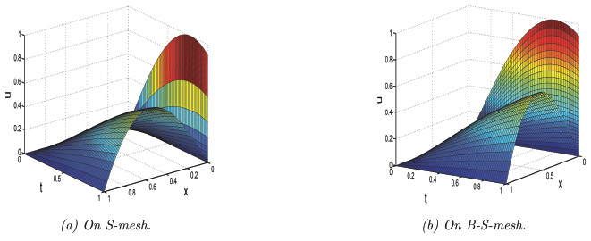
Figure 1 Numerical solution using the implicit Euler scheme for Example 5.1.

Table 1 $E_{\epsilon }^N$ and $P_{\epsilon }^N$ using the implicit Euler scheme for Example 5.1

	Number of Intervals N (Δt)
	32 (1/32)	64 (1/64)	128 (1/128)	256 (1/256)	512 (1/512)
S-mesh	1e − 4	5.0600e-03 0.7219	3.0677e-03 0.8373	1.7169e-03 0.91216	9.1234e-04 0.95546	4.7047e-04
	1e − 6	5.0776e-03 0.7220	3.0782e-03 0.8374	1.7227e-03 0.9122	9.1537e-04 0.9555	4.7201e-04
	1e − 8	5.0778e-03 0.7220	3.0783e-03 0.8374	1.7228e-03 0.9122	9.1540e-04 0.9555	4.7203e-04
B-S-mesh	1e − 4	5.3394e-03 0.7993	3.0681e-03 0.8374	1.7171e-03 0.9122	9.1238e-04 0.9554	4.7049e-04
	1e − 6	5.3448e-03 0.7960	3.0782e-03 0.8374	1.7227e-03 0.9122	9.1537e-04 0.9555	4.7201e-04
	1e − 8	5.3449e-03 0.7960	3.0783e-03 0.837	1.7228e-03 0.9122	9.1540e-04 0.9555	4.7203e-04
M-B-S-mesh	1e − 4	5.4471e-03 0.8226	3.0685e-03 0.8374	1.7173e-03 0.9122	9.1242e-04 0.9554	4.7050e-04
	1e − 6	5.4443e-03 0.8226	3.0782e-03 0.8374	1.7227e-03 0.9122	9.1537e-04 0.9555	4.7201e-04
	1e − 8	5.4442e-03 0.8226	3.0783e-03 0.8374	1.7228e-03 0.9122	9.1540e-04 0.9555	4.7203e-04

To visualize the numerical order of convergence, the maximum pointwise errors is plotted in log-log scale in Figure 2 for Example 5.1 using the implicit Euler scheme (16) on B-S-mesh. The maximum pointwise errors are plotted in log-log scale in Figure 4(e) and Figure 4(f) for Example 5.1 using implicit trapezoidal scheme(17) on S-mesh and M-B-S-mesh respectively. Figures 5(g) and 5(h) represent the numerical solution of Example 5.2 using the scheme (16) for N = 64 on S-mesh and B-S-mesh respectively. On B-S-mesh and M-B-S-mesh, the proposed numerical scheme (16) is of first order in the temporal and second order in the spatial variable, i.e., of order 𝒪(Δt + N⁻²) which is optimal for the scheme (16). While the second scheme (17) is of second order both in temporal and spatial variable i.e., of order 𝒪(Δt² + N⁻²) which is also optimal for the scheme (17). Numerical results confirm the theoretical error estimate. Hence, we have shown that the proposed scheme is a second order on both time and space without taking any restriction discussed earlier.

Table 2 $E_{\epsilon }^N$ and $P_{\epsilon }^N$ using the implicit Euler scheme for Example 5.1

	Number of Intervals N (Δt)
	32 (1/322)	64 (1/642)	128 (1/1282)	256 (1/2562)	512 (1/5122)
S-mesh	1e − 4	1.8153e-2 1.5065	6.3890e-3 1.5813	2.1351e-3 1.6023	7.0323e-4 1.6578	2.3521e-4
	1e − 6	1.8155e-2 1.5062	6.3913e-3 1.5807	2.1367e-3 1.6017	7.0405e-4 1.6567	2.3565e-4
	1e − 8	1.8155e-2 1.5062	6.3913e-3 1.5807	2.1367e-3 1.6017	7.0405e-4 1.6567	2.3565e-4
B-S-mesh	1e − 4	1.6622e-3 1.9293	4.3641e-4 1.9831	1.1039e-4 2.0115	2.7379e-5 2.0475	6.6228e-6
	1e − 6	1.6641e-3 1.9231	4.3881e-4 1.9694	1.1205e-4 1.9843	2.8321e-5 1.9921	7.1191e-6
	1e − 8	1.6641e-3 1.9233	4.3884e-4 1.9693	1.1207e-4 1.9840	2.8327e-05 1.9965	7.1240e-6
M-B-S-mesh	1e − 4	1.4020e-3 1.9836	3.5450e-4 1.9219	9.3553e-5 1.9306	2.4541e-5 1.9717	6.2568e-6
	1e − 6	1.3977e-3 1.9961	3.5036e-4 1.8756	9.5477e-5 1.8967	2.5640e-5 1.9201	6.7751e-6
	1e − 8	1.3976e-3 1.9962	3.5032e-4 1.8752	9.5494e-5 1.8964	2.5650e-5 1.9195	6.7808e-6

Table 3 $E_{\epsilon }^N$ and $P_{\epsilon }^N$ using the implicit trapezoidal scheme for Example 5.1

	Number of Intervals N (Δt)
	ε	32 (1/32)	64 (1/64)	128 (1/128)	256 (1/256)	512 (1/512)
S-mesh	1e − 4	1.8111e-2 1.5057	6.3779e-3 1.5807	2.1322e-3 1.6017	7.0256e-4 1.6575	2.2270e-4 1.6944
	1e − 6	1.8115e-2 1.5055	6.3804e-3 1.5802	2.1338e-3 1.6010	7.0338e-4 1.6564	2.2314e-4 1.6927
	1e − 8	1.8115e-2 1.5055	6.3804e-3 1.5802	2.1338e-3 1.6010	7.0338e-4 1.6564	2.2314e-4 1.6927
B-S-mesh	1e − 4	1.6183e-3 1.9293	4.2489e-4 1.9826	1.0751e-4 2.0109	2.6676e-5 2.0293	6.5351e-6 1.8433
	1e − 6	1.6203e-3 1.9228	4.2736e-4 1.9686	1.0919e-4 1.9832	2.7618e-5 1.9921	6.9422e-6 1.9969
	1e − 8	1.6203e-3 1.9227	4.2738e-4 1.9685	1.0921e-4 1.9829	2.7627e-5 1.9916	6.9470e-6 1.9958
M-B-S-mesh	1e − 4	1.4724e-3 1.9850	3.7195e-4 1.9738	9.4693e-5 1.9501	2.4506e-5 1.9075	6.5321e-6 1.8435
	1e − 6	1.4681e-3 1.9958	3.6810e-4 1.9964	9.2256e-5 1.9003	2.4714e-5 1.9239	6.5130e-6 1.9473
	1e − 8	1.4677e-3 1.9969	3.6770e-4 1.9962	9.2169e-5 1.8929	2.4817e-05 1.9176	6.5690e-6 1.9351

Table 4 Time comparison using the scheme (16) for Example 5.1

Meshes	Thomas Algorithm			Matrix Inverse Algorithm
	128	256	512	128	256	512
S-mesh	116.677	106.083	801.951	1275.027	1268.127	65293.353
B-S-mesh	266.191	186.234	1503.081	1275.027	1268.127	69493.567
M-B-S-mesh	263.086	186.789	1503.781	1275.354	1267.982	69443.367

Table 5 Time comparison using the scheme (17) for Example 5.1

Meshes	Thomas Algorithm			Matrix Inverse Algorithm
	128	256	512	128	256	512
S-mesh	0.997	4.495	22.032	5.463	169.871	3767.312
B-S-mesh	1.657	6.988	33.681	6.526	176.550	4012.327
M-B-S-mesh	1.673	7.022	33.796	6.734	176.745	4012.234

Table 6 ${\tilde{E}}_{\epsilon }^N$ and ${\tilde{P}}_{\epsilon }^N$ using the implicit trapezoidal scheme for Example 5.2

	Number of Intervals N (Δt)
	ε	32 (1/32)	64 (1/64)	128 (1/128)	256 (1/256)	512 (1/512)
S-mesh	1e − 4	5.7945e-03 1.5341	2.0009e-03 1.5981	6.6093e-04 1.6186	2.1523e-04 1.6640	6.7917e-05
	1e − 6	5.8005e-03 1.5343	2.0026e-03 1.5982	6.6144e-04 1.6190	2.1534e-04 1.6642	6.7941e-05
	1e − 8	5.8006e-03 1.5343	2.0026e-03 1.5982	6.6144e-04 1.6190	2.1534e-04 1.6642	6.7942e-05
B-S-mesh	1e − 4	9.3641e-4 1.9343	2.4501e-4 1.9760	6.2279e-5 1.9854	1.5728e-5 2.0406	3.8228e-6
	1e − 6	9.3636e-4 1.9330	2.4521e-4 1.9694	6.2262e-5 1.9848	1.5730e-5 2.0403	3.8242e-6
	1e − 8	9.3636e-4 1.9330	2.4521e-4 1.9694	6.2262e-5 1.9848	1.5730e-5 2.0403	3.8242e-6
M-B-S-mesh	1e − 4	6.3641e-4 1.9650	1.6301e-4 1.9815	4.1279e-5 2.0464	9.9928e-6 2.0442	2.4228e-6
	1e − 6	6.3661e-4 1.9628	1.6331e-4 1.9825	9.5487e-5 2.0465	2.5660e-5 2.0443	6.7791e-6
	1e − 8	6.3661e-4 1.9628	1.6331e-4 1.9825	9.5487e-5 2.0465	2.5660e-5 2.0443	6.7791e-6

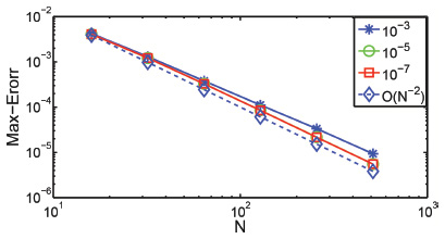
Figure 2 Loglog plot on B-S-mesh by the implicit Euler scheme for Example 5.1.

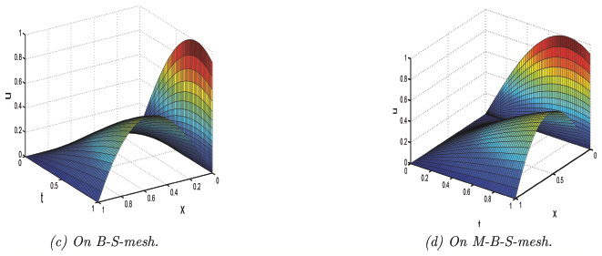
Figure 3 Numerical solution by the implicit trapezoidal scheme for Example 5.1.

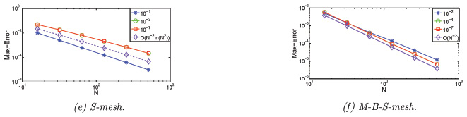
Figure 4 Loglog plot by the implicit trapezoidal scheme for Example 5.1.

In this article, we propose two numerical methods to solve one-dimensional singularly perturbed parabolic convection-diffusion problem. First, we use implicit Euler method for the temporal and a monotone hybrid scheme for the spatial variable. For the monotone hybrid scheme discussed here, the weights are so chosen that the scheme automatically switched from midpoint upwind scheme to central difference scheme as the mesh goes from coarse to fine. We obtain parameter uniform convergent solution and of order 𝒪(Δt + N⁻²). In order to increase the accuracy, we have also used the implicit trapezoidal scheme for the temporal variable which increases the order of accuracy from first order in time to second order in time 𝒪(Δt² + N⁻²). We derived ε-uniform error estimate for the proposed schemes. Also, Thomas algorithm is used which takes less time than the matrix inversion method. Numerical results are carried out to show the efficiency and accuracy of the method.

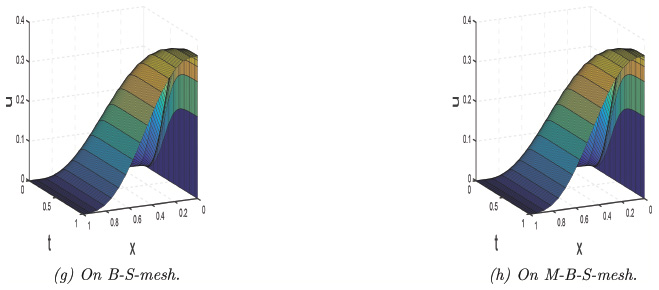
Figure 5 Numerical solution by the implicit Euler scheme for Example 5.2.

Acknowledgement

The authors express their thanks to unknown reviewers for valuable remarks and comments which improved the paper. The financial support received from SERB, Govt. of India via the research grant number EMR/2016/005805 is gratefully acknowledged.

Appendix

A similar result is established in ‘(Palencia, 1993)’ for any operator R of the form R(L_x), where R(z) is a rational A-acceptable function and L_x is any operator that generates an analytic semigroup e^−tLx. In ‘(Palencia, 1993)’, R(z) is the amplification function of the Crank-Nicolson scheme and L_x is the Laplacian operator. To prove (11), we need to show that L_x,ε is ε-uniformly sectorial. Assume that (X, ‖.‖_X) and (Y, ‖.‖_Y) be two Banach spaces and let L(X, Y) be the space of bounded linear operators from X into Y equipped with the natural norm ‖A‖_L(X,Y) = sup_x∈X,x≠0 ‖Ax‖_Y/‖X‖_X. A linear operator A : D(A) ⊂ X → X is said to be sectorial operator in X if there exits a constant w ∈ ℝ, θ ∈ (π/2, π) and M > 0 such that the following holds:

• (1) ${\displaystyle {\sum }_{\theta ,w}}:=\left\{z\in C:z\ne w,\left|\mathit{arg}(z-w)\right|<\theta \right\}\subset \rho (A)$, the resolvent set of A, and
• (2) ${\Vert {(zI-A)}^{-1}\Vert }_X\le \frac{M}{z-w}$ for $z\in {\displaystyle {\sum }_{\theta ,w}}$.

A details of this argument is given in ‘(Kumar & Sekhara Rao, 2010; Lunardi, 1995)’. If ‘A’ is sectorial, then ‘A’ generates an analytic semigroup S(t) = e^tA ∀t ≥ 0. The operator ‘A’ is said to be ?-uniformly sectorial if we choose the Banach space X equipped with the sup norm ‖.‖_∞ and the constant M is independent of ε. Let X = C(Ω) where Ω ⊂ ℝ and is equipped with the sup norm. Now consider the linear operator L_x,ε : C²(Ω) ⊂ C(Ω) → C(Ω), defined by $L_{x,\epsilon }=-\epsilon \frac{{\partial }^{2}u}{\partial x^2}-a(x)\frac{\partial u}{\partial x}+b(x)u$, which we decomposed as L_x,ε := S₁+S₂, The operator S₁ : C²(Ω) ⊂ C(Ω) → C(Ω), is defined by $S_{1}u=-\epsilon \frac{{\partial }^{2}u}{\partial x^2}$, and the operator S₂ : C(Ω) → C(Ω) is defined by $S_{2}u=-a(x)\frac{\partial u}{\partial x}+b(x)u$. The corollary (3.1.9) in ‘(Lunardi, 1995)’ with the property that sectors are invariant under the dilations gives that S₁ is ε-uniformly sectorial. Using this with S₂, ∈ L(X, X), the proposition (2.4.1) of ‘(Lunardi, 1995)’ concludes that L_x,ε is ε-uniformly sectorial, which is our desired result.

References

Andreev, V. B. & Kopteva, N. V. (1998). On the convergence, uniform with respect to a small parameter, of monotone three- point finite difference approximation. Journal of Difference Equations, 34, pp. 921–929.

Bansal, K., Rai, P. & Sharma, K. K. (2017). Numerical treatment for the class of time dependent singularly perturbed parabolic problems with general shift arguments. Differential Equations and Dynamical Systems, 25(2), pp. 327–346.

Brandt, A. & Yavneh, I. (1991). Inadequacy of first-order upwind difference schemes for some recirculating flows. Journal of Computational Physics, 93, pp. 128–143.

Clavero, C., Gracia, J. L. & Jorge, J. C. (2005). High-order numerical methods for one-dimensional parabolic singularly perturbed problems with regular layers. Numerical Methods Partial Differential Equations, 21, pp. 148–169.

Clavero, C., Jorge, J. C. & Lisbona, F. (2003). A uniformly convergent scheme on a nonuniform mesh for convection-diffusion parabolic problems. Journal of Computational Methods in Applied Mathematics, 154, pp. 415–429.

Farrell, P. A., Hegarty, A. F., Miller, J. J. H., O’Riordan, E. & Shishkin, G. I. (2000) Robust Computational Techniques for Boundary Layers. Chapman & Hall/CRC Press, Boca Raton, FL.

Gartland, E. C. (1988). An analysis of a uniformly convergence finite difference or finite element scheme for a model singular-perturbation problem. Mathematics of Computation, 51(183), pp. 93–106.

Gartland, E. C. (1988a). Graded-mesh difference schemes for singularly perturbed two-point boundary value problem. Mathematics of Computation, 51(184), pp. 631–657.

Guo, W. & Stynes, M. (1993). Finite element analysis of exponentialy fitted lumped schemes for time-dependent convection-diffusion problems. Numerische Mathematik, 66, pp. 347–371.

Kay, B. D. & Elrick, D. E. (1967). Absorption and movement of lindane in soils. Soil Science, 104, pp. 314–22.

Kellogg, R. B. & Tsan, A. (1978). Analysis of some diffenece approximations for a singularly perturbed problem without turning points. Mathematics of Computation, 32, pp. 1025–1039.

Kumar, M. & Sekhara Rao, S. C. (2010). High order parameter-robust numerical method for time dependent singularly perturbed reaction-diffusion problems. Computing, 90(1–2), pp. 15–38.

Linß, T., Roos, H.-G. & Vulanović, R. (2000). Uniform pointwise convergence on Shishkin-type meshes for quasi-linear convection-diffusion problems. SIAM Journal on Numerical Analysis, 38, pp. 897–912.

Linß, T. (2001). Sufficient conditions for uniform convergence on layer-adapted grids. Applied Numerical Mathematics, 37, pp. 241–255.

Linß, T. (2001). Uniform second-order pointwise convergence of a finite difference discretization for a quasilinear problem. Zhurnal Vychislitel’noi Matematiki i Matematicheskoi Fiziki, 41(6), pp. 947–958.

Lunardi, A. (1995). Analytic Semigroups and Optimal Regularity in Parabolic Problems. Progress in nonlinear differential equations and their applications, 16. Birkhäuser, Basel.

Kopteva, N. & Linß, T. (2001). Uniform second-order pointwise convergence of a central difference approximation for a quasilinear convection-diffusion problem. Journal of Computational Methods in Applied Mathematics, 137, pp. 257–267.

Melenk, J. M., Xenophontos, C. & Oberbroeckling, L. (2013). Robust exponential convergence of hp FEM for singularly perturbed reaction-diffusion systems with multiple scales. IMA Journal of Numerical Analysis, 33(2), pp. 609–628.

Miller, J. J. H., O’Riordan, E. & Shishkin, G. I. (2012). Fitted Numerical Methods for Singular Perturbation Problems, Revised Edition. World Scientific, Singapore.

Misra, C. & Mishra, B. K. (1977). Miscible displacement of nitrate and chloride under field conditions. Soil Science Society of America Journal, 41, pp. 496–499.

Mukherjee, K. & Natesan, S. (2009). Parameter-uniform hybrid numerical scheme for time-dependent convection-dominated initial-boundary-value problems. Computing, 84, pp. 209–230.

Ng-Stynes, M. J., O’Riordan, E. & Stynes, M. (1988). Numerical methods for time-dependent convection-diffusion equations. Journal of Computational Methods in Applied Mathematics, 21, pp. 289–310.

O’Riordan, E. & Stynes, M. (1991). A globally uniformly convergent finite element method for a singularly perturbed elliptic problem in two dimensions. Mathematics of Computation, 51, pp. 47–62.

Palencia, C. (1993). A stability result for sectorical operators in Banach spaces. SIAM Journal on Numerical Analysis, 30, 1373–1384.

Raji Reddy, N. & Mohapatra, J. (2015). An efficient numerical method for singularly perturbed two point boundary value problems exhibiting boundary Layers. National Academy Science Letters, 38(4), pp. 355–359.

Salama, A. A. & Al-Amerya, D. G. (2017). A higher order uniformly convergent method for singularly perturbed delay parabolic partial differential equations. International Journal of Computer Mathematics, 12(94), 2520–2546.

Schwab, C., Suri, M. & Xenophontos, C. A. (1996). Boundary layer approximation by spectral/hp methods. Houston Journal of Mathematics Spec. Issue of ICOSAHOM, 95, pp. 501–508.

Shishkin, G. I. & Shishkina, L. P. (2009). Difference Methods for Singular Perturbation Problems. CRC Press, Boca Raton.

Stynes, M. & Roos, H. G. (1997). The midpoint upwind scheme. Applied Numerical Mathematics, 23, pp. 361–374.

Vulanović, R. (1989). A uniform method for quasilinear singular perturbation problems without turning points. Computing, 4(1), pp. 97–106.

Vulanović, R. (2001). A priori meshes for singularly perturbed quasilinear two-point boundary value problems. IMA Journal of Numerical Analysis, 21(1), pp. 349–366.

Xenophontos, C. (1998). The h-p finite element method for singularly perturbed boundary value problems on smooth domains. Math. Models and Methods in Applied Sciences, 8, pp. 69–79.

Xenophontos, C. (1998). The h-p finite element method for singularly perturbed problems on non-smooth domains. Numerical Methods for Partial Differential Equations, 16, 1–28.

Biographies

Lolugu Govindarao received M.Sc. and M.Phil from Pondichery University, India. Currently he is pursuing Ph.D. at Department of Mathematics, National Institute of Technology Rourkela, India. His research interests include numerical methods for singular perturbation problems.

Jugal Mohapatra Ph.D. from Indian Institute of Technology Guwahati, India. He is currently working at Department of Mathematics, National Institute of Technology Rourkela. His research interest is Numerical Analysis mainly finite difference methods for singularly perturbed differential equations.

European Journal of Computational Mechanics, Vol. 28_5, 467–498.
doi: 10.13052/ejcm2642-2085.2854
© 2020 River Publishers