Material Model Calibration Using Machine Learning: A Comparative Study
Mariana Seabra* and Ana Costa
University of Porto Faculty of Engineering, Porto, Portugal
E-mail: marianas@fe.up.pt
*Corresponding Author
Received 02 March 2022; Accepted 11 April 2022; Publication 06 May 2022
Abstract
A methodology based on Machine Learning, namely Fully Connected Neural Networks, is proposed to replace traditional parameter calibration strategies. In particular, the relation between hardness, yield strength and tensile strength is explored. The proposed methodology is used to predict the yield strength and the tensile strength of a Super Duplex Stainless Steel that was not included in the neural network training data base. Moreover, it is also used to determine such material parameters for individual microstructural phases, which feed a multiscale Finite Element simulation. The methodology is experimentally validated.
Keywords: Neural network, hardness, yield strength, tensile strength, Duplex Stainless Steel.
1 Introduction
Traditionally, the design of new steel alloys and components relies on trial-error procedures, which involve exhaustive experimental testing [1]. Numerical methods, in particular the Finite Element Method (FEM) (e.g. [45, 10]) and its various developments have contributed to lessen such testing. Using FEM, service performance and/or production stages of components may be simulated in a virtual environment and optimization procedures may be executed during design stage. Nevertheless, material models used in conjunction with the FEM still require experimental calibration procedures, involving extensive work hours and generating considerable quantities of waste. Notwithstanding, a substantial amount of data regarding alloys characterization has been collected throughout the years making it possible to avoid costly experimental characterizations by combining currently available information and machine learning.
Machine learning (ML) employs algorithms and statistical models to analyze and draw inferences from patterns in data [21]. Neural Network (NN) is one of the most famous methods in this field inspired by the sophisticated functionality of human brains. In the field of Material Science, it can be used to obtain an optimal target material property without solving physical or chemical fundamental equations [29]. It substantially reduces computational costs and shortens development cycles. Additionally, it may reach a higher prediction accuracy when compared with conventional calculations based on first principles[1, 2, 29]. However, the success of this approach lies in the ability of the system to learn descriptors of data with different levels of abstraction, without human intervention, which generates a considerable degree of epistemic opacity [41]. Consequently, as the learned relations are not explicitly available to the user, NN are often used as black-boxes, which may result in mere correlations without causal significance. As a result, physics-driven information has to be incorporated with NN to ensure reliability.
The application of NN in the field of material science is fairly recent, and concerns mainly the discovery of new materials. In general, prospective chemical compositions are screened to find a target material property, such as thermal conductivity, tensile strength, corrosion resistance, and so forth [4, 38, 44]. Nevertheless, it has been reported in the literature [15, 43, 29] that pure data-driven approaches often lead to misleading conclusions or have poor predictive performance, especially when considering chemical composition alone as input. Moreover, insufficient size of the training sets, corrupted entries in the data bases, extremely high dimensional target spaces and lack of exploitation of correlations among different material properties are also pointed as causes of such ill performance. Therefore, to improve accuracy NN have been combined with other strategies: Conduit et al. [7] developed a computational tool that combines experimental data, computational thermodynamic calculations and a 2-layer NN to discover new nickel alloys; Kailkhura et al. [15] assembled simple machine learning modules and proposed a transference of learning technique from one module to the next, in order to increase control over the process; Xiong et al. [43] compared five different machine learning algorithms and used symbolic regression techniques to retrieve the explicit mathematical equations that describe the influence of each feature in the mechanical properties of steels. However, benchmarking strategies for the use of NN in material science are still lacking and little information is available on the influence of the NN hyperparameters (e. g. number of layers and nodes) in the final outcome.
In this work, instead of using NN abilities to discover a new alloy composition, the potentialities of NN are used to replace tedious experimental procedures required for material model calibration, especially when using the FEM. The final properties of an alloy depend on various factors beyond its chemical composition such as forming processes or thermal treatments. These factors may be considered exploring the relation between properties. In particular, the relation between hardening and yield strength and the relation between hardening and tensile strength are good candidates, as empirical and semi-empirical laws relating these properties have been proposed, e.g. [6, 5, 26, 23].
Hardening tests are relatively simple to execute when compared with other types of essays, such as tensile tests. Additionally, hardening tests are non-destructive, as only a small indentation is required, and thus are susceptible to be used in quality control. As a result, researchers have tried to establish a relation between hardness and other relevant material properties. Nevertheless, up to date, this relation has been searched in relatively small data sets and using relatively simple techniques such as linear regression, restricting its application to particular steel grades [26, 23, 37].
In this work, the relation between hardening and yield/tensile strength is established using NN. Different NN structures are explored in a comparative study to illustrate the influence of the various NN hyperparameters in the final result. As it will be explained in the forthcoming sections of this paper, the methodology is successful across different steel grades, performing better than the existing empirical/semi-empirical approaches.
Then, the best performing NN structures are used to calculate the yield strength and the tensile strength of a Super Duplex Stainless Steel (SDSS) that was not included in the NN training data-base, and results are experimentally validated. DSS and SDSS exhibit a favorable combination of mechanical and corrosion resistance properties due to their microstructure composed approximately by equal parts of austenite and ferrite. Notwithstanding, when DSS and SDSS are subjected to thermal cycles, secondary phases may arise, in particular the sigma phase [25, 34]. These secondary phases may detiorate the mechanical response of the material and therefore they have to be considered when characterizing the material, which is often done through multiscale FEM simulations. Here, the developed NN approach is used to replace the experimental characterization of the individual microstructural phases, which feed a multiscale FEM simulation.
As a result, the methodology developed in this work reduces the amount of experimental procedures that have to be carried every time a new alloy is developed. Moreover, it may be used to test prospect compositions prior to production. In terms of numerical simulation, it was used to retrieve the material parameters required for an elasto-plastic material model and it has the potential to be extended to other models (e.g. GTN [13, 39]), as long as the relevant data is available. Finally, this paper also contributes for the general development of the use of NN in material science by giving some hints on the influence of NN hyperparameters in the final results.
This paper is organized as follows. In Section 2 the NN approach is developed concerning theoretical aspects and the application to the particular problem of predicting yield strength and tensile strength of a steel alloy. The methodology is applied to a steel alloy not included in the training data base in Section 3 and results are experimentally validated. Finally, in Section 4 the final conclusions are outlined and future work is proposed.
2 Methods
2.1 Fully Connected Neural Network
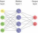
NN are one of the most used methods within the machine learning community but only in the last couple of years it became significant in the field of material science and engineering [29]. It falls in the category of supervised learning methods in which a set of labelled training data is used to find the function that connects inputs and outputs. It mimics the human brain and therefore is constituted by layers of neurons or nodes. In a fully connected network all the neurons of one layer are connected to the neurons of the subsequent layer (as schematically represented in Figure 1) and therefore such NN is structure agnostic, meaning that no particular assumptions have to be made about the inputs [16]. In this way, they constitute a good starting point for exploratory approaches and thus are employed in this work. Moreover, fully connected NN are trained in a reasonable time.
Figure 1 Scheme of a fully connected neural network (produced by the authors using latex code).
Structurally, the neurons of layer are connected to the neurons of the previous layer , through the relation:
| (1) |
where and are the vectors containing the nodal values and bias of the neurons in layers and , respectively, is the weight matrix and is the activation function. Traditionally, the Sigmoid Function is employed as activation function [18], nevertheless, it leads to vanishing gradients in the training process. Therefore, in this work the Rectified Linear Unit Function, defined as follows, is employed:
| (2) |
The weight matrices contain the parameters that have to be fitted during training, which in this work is done through the backpropagation method in a Gradient Descent fashion [27]. In brief, the output of the NN is compared with the target output, originating an error function, , which depends on the weights and biases of the network. Then, weights and biases are updated according to the following equation:
| (3) |
where and are the vectors containing all the weights and biases of the NN, at time instants and respectively, is the gradient of the error function in respect to the weights and biases vector, and is the learning rate, which, in this work, was set to 0.03. Equation (3) may be enhanced with terms depending on the previous modification values of the weights, in order to increase the convergence rate [27]. Finally, the error is evaluated through a Loss function. In this work, Smooth L1 Function was selected due to its reduced sensitivity to outliers and ability to prevent exploding gradients, when compared to alternatives [12]. It is defined as follows:
| (4) |
where and are the vectors containing the actual output and the predicted output, respectively, is a hyperparameter, that was set equal to the learning rate, .
Besides the Loss functions, which is used in the backpropagation algorithm, further metrics may be used to evaluate the performance of a NN. In this work, three additional metrics were selected, namely, Root Mean Square Error (RMSE), Mean Absolute Error (MAE) and R-squared Score (R2 Score).
RMSE is given by the following equation:
| (5) |
again, and are the vectors containing the actual output and the predicted output, respectively, and is the number of samples. RMSE is a measure of how concentrated the data is around the line of best fit. On the other hand, MAE is simply the mean deviation of all samples:
| (6) |
Finally, R2 Score measures the percentage of correct predictions given by the model:
| (7) |
where is the mean of all actual values. These three metrics are used to find an optimal network structure for the problem in hands, that is, to calculate yield/tensile strength of a material given its hardness and chemical composition.
2.2 Applying NN to Model the Relation Between Hardness and Yield/Tensile Strength
The development of a NN for a particular problem concerns the choice of several hyperparameters as outlined in Section 2.1. As referred, the Rectified Linear Unit Function was chosen as activation function, the Smooth L1 Function was chosen as Loss function and RMSE, MAE and R2 Score were selected as further metrics. Still, the hyperparameters related to structure the NN have to be set, namely the number of layers and the number of neurons in each layer. There is no unified way to define a good structure, as it depends strongly on the problem to solve. Therefore, the problem context is presented in the following section.
2.2.1 Modeling the relation between hardness and yield/tensile strength
The simplicity of execution of hardening tests has been one of the main reasons for searching a relation between hardness and other mechanical properties, in particular yield strength and tensile strength. Cahoon et al. [6, 5] proposed the following law to calculate the yield strength, , as a function of hardness, :
| (8) |
where is the strain-hardening exponent, which may be retrieved from uniaxial tensile tests or from Meyers index of empirical methods [36]. In terms of tensile strength, TS, the relation reads:
| (9) |
This method is particularly good for ferritic steels reaching an accuracy of 2%, nevertheless it looses performance in other grades.
Alternatively, Pavlina and Tyne [26] have proposed a linear relation between hardness and tensile strength, based on least-squares linear regression for a data collection of 165 points:
| (10) |
which performs well for non-austenitic hypoeutectoid steels. Finally, Rodriguez et al. [28] have updated the values of the slope and intercept of the aforementioned linear relation, when nano-hardness tests are used instead of regular hardness tests.
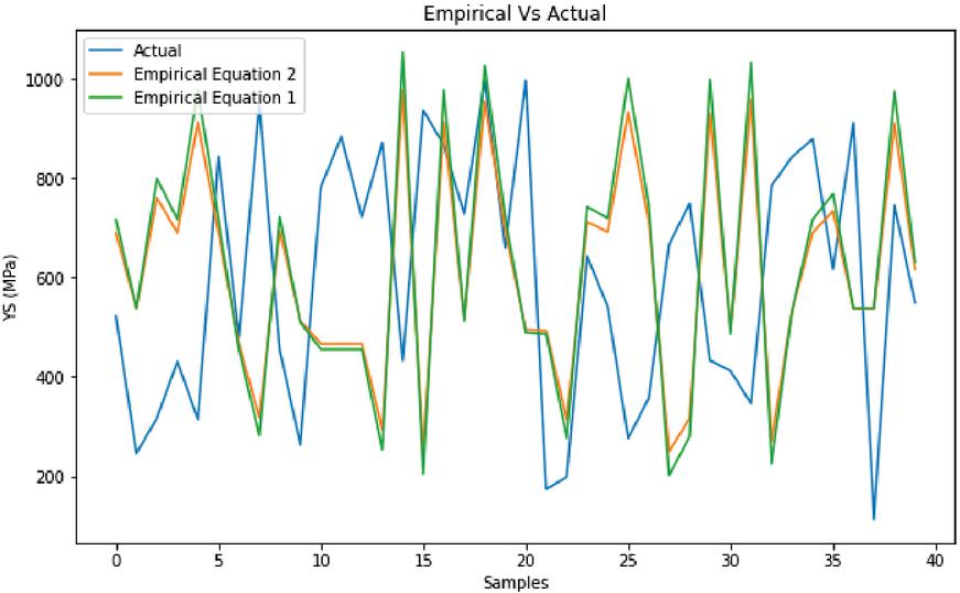
One of the main drawbacks of the stated empirical relation is their limited applicability to particular steel grades. It is difficult to compare results with the existing literature due to the difficulty in recovering the data bases used in different works. Notwithstanding, for illustration purposes, YS was calculated using Equations (8) and (10) for a random selection of 40 different steel alloys of the data base used in this work (Section 2.2.2) and plotted against the tabled values in Figure 2.
Figure 2 Measured and calculated values of the yield strength of a random sample of 40 steel alloys, using equations 8 (Empirical Equation 1) and 10 (Empirical Equation 2).
The yield strength is related to the presence strengthening alloying elements in solid solution, however most empirical equations are provided for low alloy carbon steels, loosing performance for high alloy steels, which explains the differences shown in Figure 2.
Acknowledging the importance of alloying elements is essential to model the relation between hardness and yield/tensile strength. As a result, the inputs and outputs of the NN were selected accordingly. Additionally, in order to have a better control on the performance of the NN model, yield strength and tensile strength were handled separately. Thus, two families of NN were created in this work, the first one has as inputs hardness and weight percentage of the various alloying elements, namely C, Si, Mn, P, S, Cr, Mo, Ni, N, Cu, W, V, Be, Fe, Nb, Ti, Al, Cu, La, Ce, Zr and Mg, and yield strength as output; the second family has the same inputs and tensile strength as output.
2.2.2 Data set
An adequate data set is essential for the success of fully connected neural networks training under backpropagation algorithms. Therefore, a data base containing chemical composition, hardness, yield strength and tensile strength for different steel alloys was compiled. Data was retrieved from the website steel-grades.com [30]. Corrupted entries in the data base are one of the main sources of failure, therefore, the data base was manually inspected before use, resulting in 70 different steel alloys. From the total number of data points, 80% was used to training. Subsequently, the remaining 20% were used in an inference step, where the calculated values were compared with the actual values, using the selected metrics. As the data base is relatively small, training included over-sampling, that is, some of the data points were showed more than once to the NN, resulting in a total of 200 data points. It has been demonstrated that this procedure improves training speed and generalization abilities of NN [31].
2.2.3 Network structure
After defining inputs and outputs and collecting data, the structure of the hidden layers of the NN has to be defined. Although there are some techniques which can aid in the optimization of the hyperparameters (e.g. dropout [35], batch normalization [14]), a departure structure is in general determined by trial-error, especially in fields where the use of NN is still under development. Therefore, in this work, the number of hidden layers was added iteratively, until a reasonable performance was achieved.
The performance of each NN is evaluated through the values of the loss function and the values of the selected metrics, defined in Section 2.1. The loss function is evaluated in the training and inference steps, while the remaining metrics are only evaluated in the inference step. Results for each particular NN structure are displayed in Tables 1 and 2, regarding yield strength and tensile strength, respectively.
Table 1 NN metrics when calculating yield strength. Each NN structure is defined by the number of hidden layers/total number of hidden neurons. Training consisted of 80% of data and the remaining 20% was used for inference
| Training | Inference | RMSE | MAE | R2 | |
| NN Structure | Loss (MPa) | Loss (MPa) | (MPa) | (MPa) | Score |
| 2/96 | 35 | 46 | 101 | 46 | 0.843 |
| 3/112 | 25 | 39 | 95 | 40 | 0.862 |
| 3/224 | 19 | 33 | 67 | 33 | 0.931 |
| 4/240 | 22 | 34 | 72 | 34 | 0.920 |
| 4/120 | 29 | 32 | 60 | 32 | 0.944 |
| 5/248 | 36 | 40 | 72 | 40 | 0.898 |
Table 2 NN metrics when calculating tensile strength. Each NN structure is defined by the number of hidden layers/total number of hidden neurons. Training consisted of 80% of data and the remaining 20% was used for inference
| Training | Inference | RMSE | MAE | R2 | |
| NN Structure | Loss (MPa) | Loss (MPa) | (MPa) | (MPa) | Score |
| 3/224 | 29 | 48 | 119 | 49 | 0.774 |
| 4/240 | 36 | 49 | 114 | 50 | 0.793 |
| 4/120 | 44 | 63 | 107 | 63 | 0.818 |
| 5/248 | 32 | 52 | 126 | 53 | 0.749 |
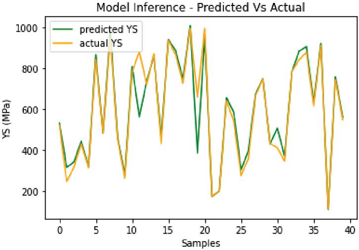
Figure 3 Yield Strength of different steel grades calculated by NN 4HL/240HN and respective tabled values.
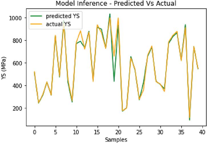
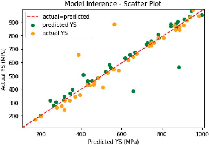
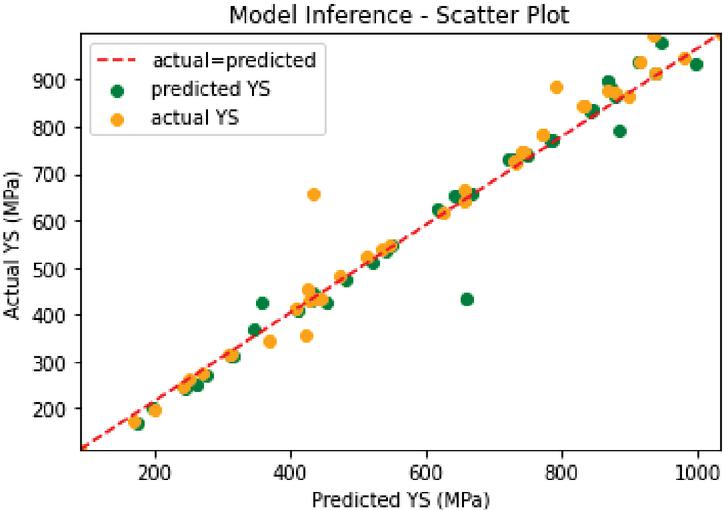
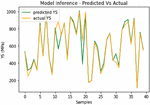
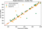
In terms of yield strength, NN 3 hidden layers (HL) and 224 hidden neurons (HN) neurons, NN 4HL/240HN and NN 4HL/120HN exhibited the best performance. In NN 3HL/224HN inference loss is significantly larger than its training loss, which may suggest that this NN tends to memorize the database, loosing generalization power, while NN 4HL/120HN exhibits slightly better metrics than the other two. Adding one addtional hidden layer worsens the results, suggesting that 4 hidden layers is the optimal number of layers for this problem. The calculated value of the yield strength during the inference stage is plotted against the actual value in Figures 3 and 4 for NN 4HL/240HN and NN 4HL/120HN, respectively. In Figures 5 and 6 results are displayed in scatter form.
Figure 4 Yield Strength of different steel grades calculated by NN 4HL/120HN and respective tabled values.
Figure 5 Scatter of calculated yield Strength of different steel grades using NN 4HL/240HN.
Figure 6 Scatter of calculated yield Strength of different steel grades using NN 4HL/120HN.
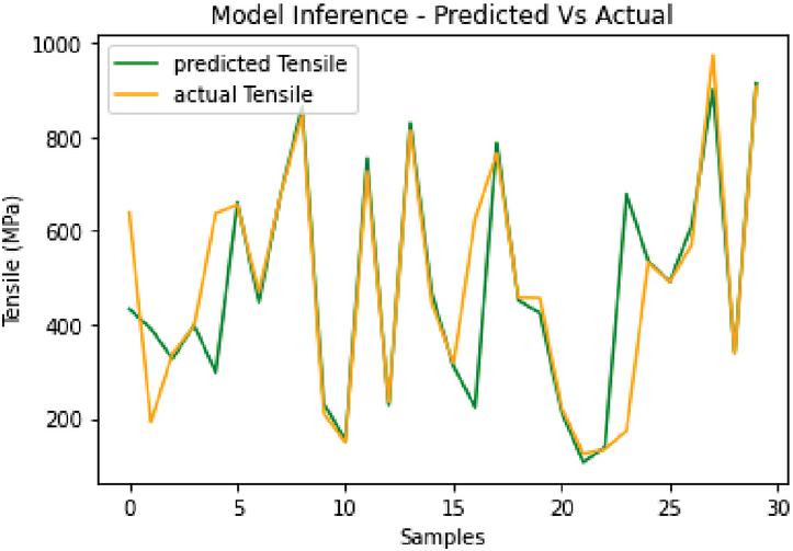
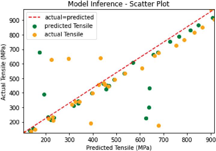
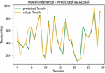
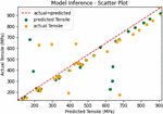
In terms of tensile strength, the results were less good, but still satisfactory, as tensile strength was correctly predicted for approximately 80% of the data points not used for training. NN 4HL/120HN exhibited the best performance and thus its results are displayed in graphic form in Figures 7 and 8.
Figure 7 Tensile strength of different steel grades NN 4HL/120HN.
Figure 8 Tensile strength of different steel grades NN 4HL/120HN. Results are displayed in the scatter form.
Table 3 NN Metrics when calculating tensile strength. Each NN structure is defined by the number of hidden layers/total number of hidden neurons. Training consisted of 85% of data and the remaining 15% was used for inference
| Training | Inference | RMSE | MAE | R2 | |
| NN Structure | Loss (MPa) | Loss (MPa) | (MPa) | (MPa) | Score |
| 3/224 | 45 | 70 | 122 | 71 | 0.748 |
| 4/224 | 46 | 65 | 115 | 65 | 0.777 |
| 4/120 | 33 | 67 | 144 | 68 | 0.648 |
| 5/248 | 35 | 60 | 137 | 60 | 0.684 |
An additional strategy to improve a NN performance is the increase of training time. Therefore, as an attempt to improve the calculation of tensile strength, the most promising NN structures were retrained using an additional 5% of data and results are displayed in Table 3. NN 4HL/120HN significantly lost performance, that is, lost ability to accommodate new data points. On the contrary, NN 4HL/240HN showed approximately the same performance, indicating a good generalization ability for new data. This NN has more hidden nodes than data points provided during training, which is often beneficial as it has been reported in the literature [20, 19]. Backpropagation training algorithms often result in sub-optimal solutions. The extra degrees of freedom can aid convergence as they decrease the chance of being stuck in local minima, when updating the network weights. Consequently, NN are not as prone to over-fitting as conventional types of interpolation, such as polynomial interpolation. Nevertheless, there is still a trade-off between over-fitting and poor approximation. The worst performance of the NN with 5 hidden layers is a indicator that over-fitting may be occurring. As a result, the NN with 4 hidden layers and a total of 240 nodes exhibited the overall best performance.
In the following section, the developed NN strategy is applied to the characterization of the mechanical behaviour of a particular still alloy, not included in the training or inference sets.
3 Results
In this section, the NN strategy developed in Section 2 is used to characterize the mechanical properties of SDSS 25Cr-7Ni-Mo-N. Casting DSS and SDSS have received less attention in the literature, when compared to wrought DSS and SDSS [17, 34]. As cast SDSS and DSS are still in a characterization stage, they are one of the material classes that may take significant advantages from the proposed methodology. Firstly, the bulk material is characterized in Section 3.1 and next, in Section 3.2, the material is characterized in microstructural terms, employing a multisclale FEM simulation.
3.1 Bulk Material
SDSS 25Cr-7Ni-Mo-N was not part of the training set or inference set of the developed NN. Therefore, the best performing networks defined in Section 2.2.3 are used to predict the yield strength and tensile strength of this material, given its chemical composition and hardness. The chemical composition is presented on Table 4, while hardness was experimentally measured as 279 HV, through a standard Vickers test HV 20. Calculated values for the yield strength and tensile strength are displayed on Table 5 and compared with the actual values of MPa and MPa. The actual values were experimentally determined in a tensile test, whose details are provided in Section 3.2.2.
Table 4 Chemical composition of the 25Cr-7Mo-Ni-N SDSS (wt%)
| C | Si | Mn | Ni | Mo | Cr | Cu | W | N |
| 0.02 | 0.7 | 0.7 | 7.9 | 3.8 | 25.3 | 0.9 | 0.7 | 0.2 |
Table 5 Calculated values of the yield strength and the tensile strength of SDSS 25Cr-7Ni-Mo-N and relative error in respect of the actual value, which was experimentally determined
| Yield | Relative | Tensile | Relative | |
| NN Structure | Strength (MPa) | Error % | Strength (MPa) | Erros % |
| 3/224 | 542 | 1.3 | 896 | 1.2 |
| 4/224 | 561 | 2.2 | 902 | 0.6 |
| 4/120 | 546 | 0.6 | 915 | 0.9 |
| 5/248 | 529 | 3.6 | 887 | 2.2 |
All selected NN were able to calculate the yield strength and the tensile strength of SDSS 25Cr-7Ni-Mo-N with good accuracy. In particular, NN with 4 hidden layers exhibited the best performance, as it was expected considering the analysis presented in Section 2.2.3. Next, the developed NN approach is used to determine the yield strength and tensile strength of the individual microstructural phases of SDSS 25Cr-7Ni-Mo-N.
3.2 SDSS Microstructure
It is well known that mechanical properties of DSS and SDSS are dependent on the amount of secondary phases [24, 17, 34]. Nevertheless, such dependence is specific for each particular alloy. Different chemical compositions combined with particular thermal cycles lead to different stereological parameters (e.g. grain size, distribution of microstructural phases), therefore, a relation between micro-properties and macro-properties has to be established. The Representative Volume Element (RVE) [3, 11] has been one of the leading approaches in this respect and thus it is applied in this work. As it requires the identification of the yield strength of individual phases, NN are applied for this purpose in Section 3.2.1. Section 3.2.2 furnishes the details of the experimental tensile essay, and finally in Section 3.2.3 the RVE based FEM multiscale simulation is compared with the experimental tensile curve.
3.2.1 Mechanical properties of ferrite, austenite and sigma
The neural network with 4 hidden layers and 240 hidden nodes was used to calculate the yield strength of ferrite (-phase), austenite (-phase) and sigma phase (-phase). This NN was selected due to its overall good performance. The chemical composition of each individual phase was obtained through SEM-EDS, as part of a thesis work within the project this paper is inserted [33]. It is presented in Table 6. Element C was also considered as input and was obtained calculating the difference to 100% from the other elements. Hardness was measured through micro-indentation tests, employing a load of 25gf. Results are displayed in Table 7.
Table 6 Chemical composition of each individual phase (wt%) obtained by SEM-EDS
| Phase | Fe | Cr | Ni | Mo | W | Mn | Cu | Si |
| -phase | 60.0 | 23.0 | 9.3 | 3.3 | 1.3 | 0.7 | 1.6 | 0.9 |
| -phase | 59.8 | 26.7 | 5.1 | 4.4 | 1.6 | 0.4 | 1.0 | 1.0 |
| -phase | 53.1 | 29.3 | 4.7 | 8.0 | 2.6 | 0.4 | 0.6 | 1.2 |
Table 7 Hardness measure and calculated value for the yield strength of each individual phase
| Phase | Hardness (HV) | Calculated Yield Strength (MPa) |
| -phase | 332 | 714 |
| -phase | 387 | 640 |
| -phase | 558 | 1313 |
The values obtained for the yield strength of each individual phase are similar to the ones obtained by reference [23]. Although they were not experimentally determined, they feed a multiscale FEM simulation, which reproduced well the experimental stress-strain curve, as explained in the following sections.
3.2.2 Tensile test
The yield strength and the tensile strength of casting SDSS 25Cr-7Ni-Mo-N were experimentally determined through a tensile test. In the following paragraphs the essential features of the essay are provided. The detailed experimental procedures related to this work will be presented in a dedicated forthcoming paper by the same authors.
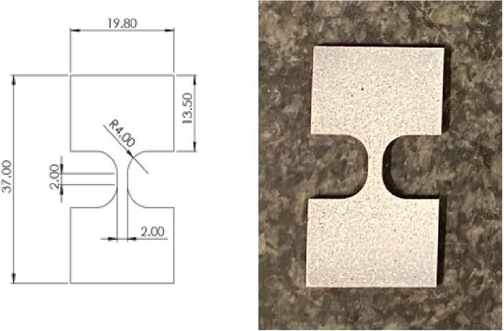
Specimens were extracted from a cast part, cutting on a milling machine, grounding and cutting by EDM. Their dimensions are shown in Figure 9. Their thickness is approximately 1.5 mm and their uniform zone measures 22 mm.
Figure 9 a – Dimensions of specimens, b – Specimens
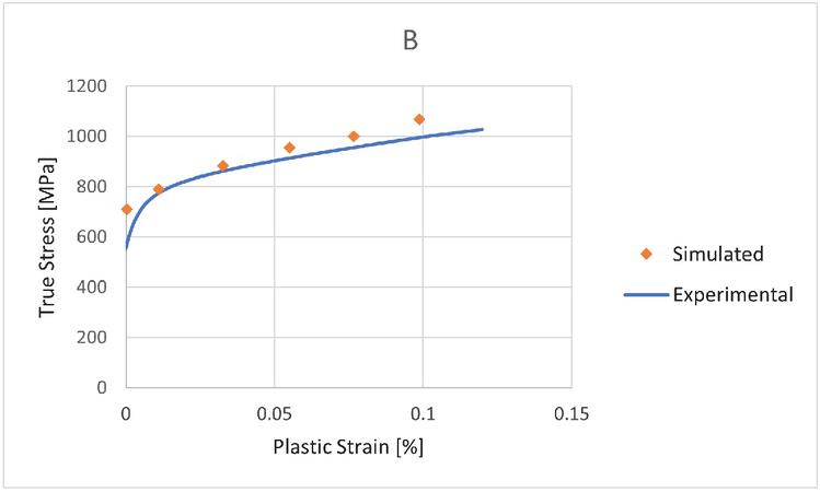
Real extension of the specimens was measured by image correlation with software V IC-2D TM (parameters displayed on Table 8). Thus, specimens were painted in white color and speckle. The machine used for the test was a prototype developed in U. Porto and INEGI especially for mini specimens [9]. The capacity of test equipment is 2,5 KN, and the test speed was set to 1 mm/min. Results are presented in Table 9 and the curve is displayed in Figure 14.
Table 8 Parameters software V IC-2D
| Correlation criteria | Normalizes Squared Differences |
| Interpolation method | Optimized 8-tap |
| Subset weights | Gaussian |
| Subset size | 29 pixel |
| Seteup size | 5 pixel |
| Low-pass filter images | yes |
| Incremental correlation | yes |
| Maximum pixel confidence | 0,05 pixel |
| Epipolar threshold | 0,5 pixel |
Table 9 Tensile test results: young modulus, yield strength, tensile strength, uniform elastic elongation, uniform plastic elongation and total elongation
| Results | |
| E (MPa) | 170 |
| YS (MPa) | 549 |
| TS (Mpa) | 907 |
| e0 (%) | 0.5 |
| eu (%) | 13.3 |
| et (%) | 26.9 |
3.2.3 Multiscale FEM simulation
In this section a RVE approach [3, 11, 8] is used to relate micro-properties and macro-properties of the SDSS 25Cr-7Ni-Mo-N. As previously referred, the optimal properties of SDSS and DSS are due to the duplex microstructure of austenite and ferrite, which is affected by the presence of the sigma phase. However, the length-scale of loads to which a SDSS is subjected is significantly larger than the characteristic length-scale of these microstructural features. Therefore, the macro behaviour of SDSS and DSS may be determined by solving a fine-scale problem over a region that contains enough statistical information about the heterogeneous medium, that is, over the Representative Volume Element (RVE).
In this work, a three step approach was used to determine the macro behaviour of SDSS 25Cr-7Ni-Mo-N. The first step consists of discretizing the RVE in a finite element mesh that can be used by commercial software Abaqus [32]. Secondly, the micro problem is solved with this software, and finally an homogenization step is taken to retrieve the macro behavior.
RVE finite element mesh
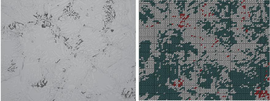
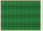
The RVE for this particular problem was generated from optical micrographs (OM), using an in-house image segmentation software [42] coded in Matlab [22]. Two threshold values are defined in the grey scale of the OM, the lowest corresponds to the limit of the -phase, and the highest to the limit of the -phase. Then the relevant micrograph is divided in a structured mesh of triangular elements, and according to the number of pixels below each threshold, a new color is attributed to the triangular element. Therefore, elements having the highest number of pixels below the first threshold are colored red, corresponding to the -phase, elements having the highest number of pixels between both thresholds are colored green, corresponding to the -phase and the remaining elements are colored grey, corresponding to the -phase. The optical micrograph and the respective RVE finite element mesh used in this work are displayed in Figure 10 (dimensions: 864 648 ). A bright -phase, a light-grey -phase, and dark-grey particles of can be observed, corresponding, respectively to grey, green and red finite elements.
Figure 10 Optical microscopy image of SDSS 25Cr-7Ni-Mo-N and respective RVE finite element mesh.
Subsequently, the created mesh is imported to Abaqus through a Python script [40], which creates typical FEM matrices with nodal coordinates and nodes belonging to each element. An additional name tag accompanies each element, which in the original mesh corresponds to one of the colors (red, green or grey) and in the new mesh corresponds to a material group (sigma, ferrite and austenite).
Micro-Problem
After importing the finite element mesh, constituted of 7200 elements, Abaqus is used to solve the elasto-plastic micro problem. Element type CPS3 was selected, and plastic behavior was modelled through a power law, as follows:
| (11) |
where , represents the real stress, represents the yield stress, represents the hardening constant, represents the real strain and represents the hardness exponent. was set to 1400, according to reference [2] for stainless steel, and the hardening exponent was set to 0.6, which is accordance with the experimental curve. The remaining material parameters are presented in Table 10, recalling that the values for the yield strength were calculated using the NN approach. Young modulus and poisson coefficient were taken from reference [23].
Table 10 Material parameters used in the FEM simulation
| Phase | Young’s Modulus (GPa) | Poisson’s Ratio | Yield Strength (MPa) |
| -phase | 189 | 0.3 | 714 |
| -phase | 220 | 0.3 | 640 |
| -phase | 201 | 0.3 | 1313 |
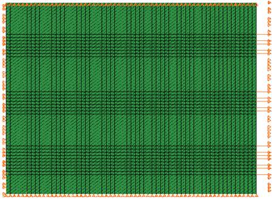
Figure 11 Boundary conditions imposed to the RVE.
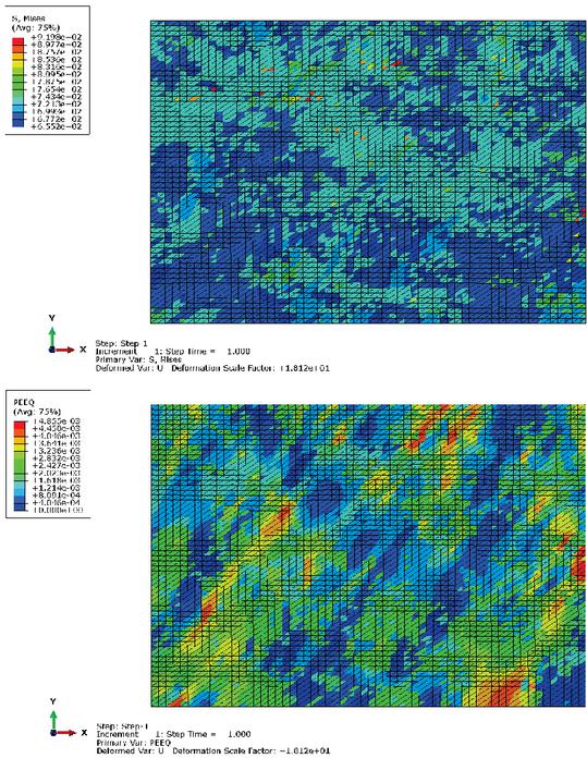
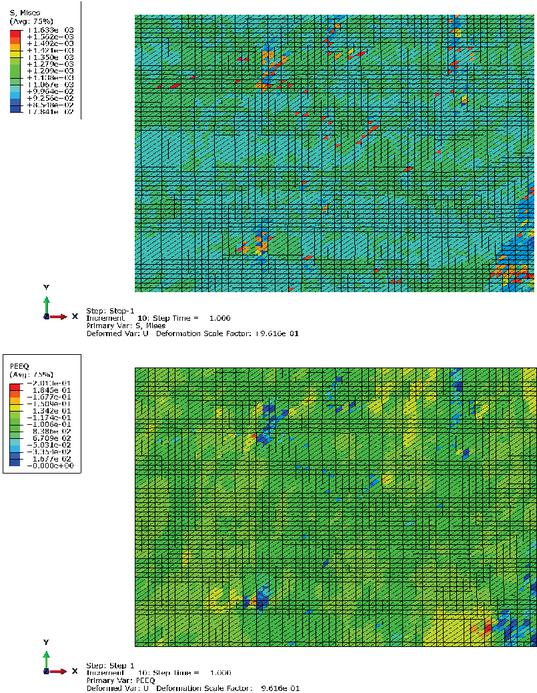
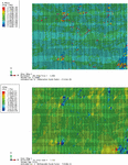
After homogenization, each micro-problem will correspond to a point in the macro tensile curve. Therefore, six different micro problems were solved, under plane stress assumption. For each problem a dislocation was imposed in the direction of the tensile test, as depicted in Figure 11. Results for the first and the last micro problems are displayed in Figures 12 and 13, where dislocations of 4.7 and 88.0 have been applied, respectively.
Figure 12 Von Mises stress and equivalent plastic strain for the first micro problem.
Figure 13 Von Mises stress and equivalent plastic strain for the last micro problem.
Figure 14 Tensile test.
Homogenization
The transition from the micro problem to the macro problem is done assuming an uniform essential boundary condition by which the micro problem displacement corresponds to the macro problem displacement, obtained by integrating the macro strain. This choice has proven to be successful in a similar analysis performed by Tao et al. [37], although it excluded the presence of sigma phase.
Macro stress, , corresponding is obtained by homogenizing the von Mises stresses of the micro problem , collected at each gauss point, as follows:
| (12) |
where and correspond to weight and jacobian of each gauss point, is total number of gauss points and is the volume of the RVE. This calculation in performed with Matlab, using the outputs written in the .obd file from Abaqus. Finally, the macro strain-stress points are compared with the experimental curve in Figure 14. There is a good correlation between numerical and experimental results, showing that the NN approach was successful in predicting the material parameters required for the multiscale elastoplastic simulation.
4 Conclusions
The NN model developed in this work predicted successfully the yield strength and tensile strength based on chemical composition and hardness of various steel alloys. In general, the overall performance was superior to the existing empirical laws, independently of the steel grade.
Different NN structures were tested and the best results were obtained when using 4 hidden layers and a number of hidden neurons slightly superior to the number of data points. In particular, the NN with a total o 240 hidden nodes was able to capture the non-linearities associated with the problem and generalize well for new data. A higher number of hidden layers seemed to lead to over-fitting.
The implemented NN strategy was able to predict accurately the yield strength and tensile strength of the cast SDSS 25Cr-7Ni-Mo-N, which was not including in the training data base of the NN. Additionally, it was adequate to determine the material properties of individual microstructural phases. Thus, results indicate that NN may be used to replace experimental characterization procedures, for both bulk material and microstructure.
The parameters calculated by the NN fed a multiscale FEM simulation, which correlated well with experiments. A simple elastoplastic model based on a power law was employed, however results suggest that other material models could benefit from this approach. The main difficulty in extending the proposed approach to more complex material models is the collection of data. As most authors publish parameters for only one particular alloy, each paper has to be screened individually in order to construct a data base.
Therefore, one of the main future tasks is the extension of the data base used in this work. Additionally, feature selection techniques will be employed to determine which of the inputs are most determinant for the output.
Acknowledgements
Authors gratefully acknowledge the funding of Project NORTE-01-0145-FEDER-032419 – msCORE – Multiscale methodology with model order reduction for advanced materials and processes, co-financed by Programa Operacional Regional do Norte (NORTE2020), through Fundo Europeu de Desenvolvimento Regional (FEDER) and by Fundação para a Ciência e Tecnologia through its component of the state budget. They also acknowledge the funding of the doctoral grant 2021.05067.BD by Fundação para a Ciência e Tecnologia, through the national budget and Community budget from European Social Fund (ESF).
References
[1] The high-throughput highway to computational materials design.
[2] I Arrayago, E Real, and Leroy Gardner. Description of stress–strain curves for stainless steel alloys. Materials & Design, 87:540–552, 2015.
[3] T Belytschko and R. de Borst. Multiscale methods in computational mechanics. Int. J. Numer. Meth. Eng, pages 939–1271, 2010.
[4] Giorgos Borboudakis, Taxiarchis Stergiannakos, Maria Frysali, Emmanuel Klontzas, Ioannis Tsamardinos, and George E Froudakis. Chemically intuited, large-scale screening of mofs by machine learning techniques. npj Computational Materials, 3(1):1–7, 2017.
[5] JR Cahoon. An improved equation relating hardness to ultimate strength. Metallurgical and Materials Transactions B, 3(11):3040–3040, 1972.
[6] JR Cahoon, WH Broughton, and AR Kutzak. The determination of yield strength from hardness measurements. Metallurgical transactions, 2(7):1979–1983, 1971.
[7] BD Conduit, Nick G Jones, Howard J Stone, and Gareth John Conduit. Design of a nickel-base superalloy using a neural network. Materials & Design, 131:358–365, 2017.
[8] APO Costa, RO Sousa, LMM Ribeiro, AD Santos, and JMA César de Sá. Multiscale modeling for residual stresses analysis of a cast super duplex stainless steel. Materials Design and Applications III, pages 47–63, 2021.
[9] Daniel Jácome da Cruz. Ensaios mecânicos de tração-compressão em provetes metálicos miniaturizados desenvolvimento de um equipamento especializado. 2019.
[10] Eduardo A de Souza Neto, Djordje Peric, and David RJ Owen. Computational methods for plasticity: theory and applications. John Wiley & Sons, 2011.
[11] Jacob Fish. Practical multiscaling. John Wiley & Sons, 2013.
[12] Ross Girshick. Fast r-cnn. In Proceedings of the IEEE international conference on computer vision, pages 1440–1448, 2015.
[13] A. L. Gurson. Continuum theory of ductile rupture by void nucleation and growth: Part I-Yield criteria and flow rules for porous ductile media. J. Engng.Mat. Tech,, 99:2–15, 1977.
[14] Sergey Ioffe and Christian Szegedy. Batch normalization: Accelerating deep network training by reducing internal covariate shift. In International conference on machine learning, pages 448–456. PMLR, 2015.
[15] Bhavya Kailkhura, Brian Gallagher, Sookyung Kim, Anna Hiszpanski, and T Han. Reliable and explainable machine-learning methods for accelerated material discovery. npj Computational Materials, 5(1):1–9, 2019.
[16] Aarti M Karande and DR Kalbande. Weight assignment algorithms for designing fully connected neural network. International Journal of Intelligent Systems and Applications, 10(6):68, 2018.
[17] Yoon-Jun Kim. Phase transformations in cast duplex stainless steels. Technical report, Ames Lab., Ames, IA (United States), 2004.
[18] John F Kolen and Stefan C Kremer. A field guide to dynamical recurrent networks. John Wiley & Sons, 2001.
[19] Ben Kröse, Ben Krose, Patrick Van der Smagt, and Patrick Smagt. An introduction to neural networks. 1993.
[20] Steve Lawrence, C Lee Giles, and Ah Chung Tsoi. Lessons in neural network training: Overfitting may be harder than expected. In AAAI/IAAI, pages 540–545. Citeseer, 1997.
[21] Pierre Lison. An introduction to machine learning. Language Technology Group (LTG), 1(35):1–35, 2015.
[22] MATLAB. version 7.10.0 (R2010a). The MathWorks Inc., Natick, Massachusetts, 2010.
[23] C Meena and V Uthaisangsuk. Micromechanics based modeling of effect of sigma phase on mechanical and failure behavior of duplex stainless steel. Metallurgical and Materials Transactions A, 52(4):1293–1313, 2021.
[24] J-O Nilsson. Super duplex stainless steels. Materials science and technology, 8(8):685–700, 1992.
[25] J-O Nilsson, P Kangas, A Wilson, and T Karlsson. Mechanical properties, microstructural stability and kinetics of -phase formation in 29cr-6ni-2mo-0.38 n superduplex stainless steel. Metallurgical and materials Transactions A, 31(1):35–45, 2000.
[26] EJ Pavlina and CJ Van Tyne. Correlation of yield strength and tensile strength with hardness for steels. Journal of materials engineering and performance, 17(6):888–893, 2008.
[27] Ning Qian. On the momentum term in gradient descent learning algorithms. Neural networks, 12(1):145–151, 1999.
[28] R Rodrıguez and I Gutierrez. Correlation between nanoindentation and tensile properties: influence of the indentation size effect. Materials Science and Engineering: A, 361(1-2):377–384, 2003.
[29] Jonathan Schmidt, Mário RG Marques, Silvana Botti, and Miguel AL Marques. Recent advances and applications of machine learning in solid-state materials science. npj Computational Materials, 5(1):1–36, 2019.
[30] S&G. Steel grades, 2021 [Online].
[31] Andrew JR Simpson. Over-sampling in a deep neural network. arXiv preprint arXiv:1502.03648, 2015.
[32] Michael Smith. ABAQUS/Standard User’s Manual, Version 6.9. Dassault Systèmes Simulia Corp, United States, 2009.
[33] Ricardo Sousa. Phase Transformations and Modelling of Thermal Stresses in a Cast Super Duplex Stainless Steel. PhD thesis, University of Porto, Faculty of Engineering, 2021.
[34] RO Sousa, P Lacerda, PJ Ferreira, and LMM Ribeiro. On the precipitation of sigma and chi phases in a cast super duplex stainless steel. Metallurgical and Materials Transactions A, 50(10):4758–4778, 2019.
[35] Nitish Srivastava. Improving neural networks with dropout. University of Toronto, 182(566):7, 2013.
[36] David Tabor. A simple theory of static and dynamic hardness. Proceedings of the Royal Society of London. Series A. Mathematical and Physical Sciences, 192(1029):247–274, 1948.
[37] Ping Tao, Jian-ming Gong, Yan-fei Wang, Yong Jiang, Yang Li, and Wei-wei Cen. Characterization on stress-strain behavior of ferrite and austenite in a 2205 duplex stainless steel based on nanoindentation and finite element method. Results in Physics, 11:377–384, 2018.
[38] Sherif Abdulkader Tawfik, Olexandr Isayev, Michelle JS Spencer, and David A Winkler. Predicting thermal properties of crystals using machine learning. Advanced Theory and Simulations, 3(2):1900208, 2020.
[39] V. Tvergaard and A. Needleman. Analysis of the cup-cone fracture in a round tensile bar. Acta Metallurgica, 32(1):157–169, 1984.
[40] Guido Van Rossum and Fred L Drake Jr. Python reference manual. Centrum voor Wiskunde en Informatica Amsterdam, 1995.
[41] Alfredo Vellido, José David Martín-Guerrero, and Paulo JG Lisboa. Making machine learning models interpretable. In ESANN, volume 12, pages 163–172. Citeseer, 2012.
[42] João Pedro Portella Guedes Visconti. A simple image segmentation approach to overcome microstructure analysis and homogenization problems. to decide, 2021.
[43] Jie Xiong, TongYi Zhang, and SanQiang Shi. Machine learning of mechanical properties of steels. Science China Technological Sciences, 63(7):1247–1255, 2020.
[44] Qionghua Zhou, Shuaihua Lu, Yilei Wu, and Jinlan Wang. Property-oriented material design based on a data-driven machine learning technique. The journal of physical chemistry letters, 11(10):3920–3927, 2020.
[45] Olek C Zienkiewicz, Robert L Taylor, and Jian Z Zhu. The finite element method: its basis and fundamentals. Elsevier, 2005.
Biographies

Mariana Seabra is an Invited Auxiliary Professor at the Faculty of Engineering, University of Porto. Her research career has been devoted to numerical methods, in particular the Finite Element Method applied to ductile damage, fracture and fatigue problems. More recently it has been focused on machine learning methods and its application to structural mechanics and material science. She is also a member of the LAETA research group.

Ana Costa is a PhD student at the Faculty of Engineering, University of Porto, working on material science, machine learning methods and its application to structural mechanics. Her research career started as a volunteer work at a physics laboratory and, later, in a mechanical construction materials laboratory. During her degree period, she also worked as an intern at FCA Fiat Chrysler Automóveis. Finally, she enrolled the project of Multi-Scale Methodologies with Order Reduction Models for Advanced Materials and Processes as a research fellow at INEGI during her master’s degree.
European Journal of Computational Mechanics, Vol. 31_1, 127–154.
doi: 10.13052/ejcm2642-2085.3115
© 2022 River Publishers

