Computation of Second-order Design Sensitivities for Steady State Incompressible Laminar Flows Using the Extended Complex Variables Method

Mahdi Hassanzadeh

Department of Mechanical Engineering, Gorgan Branch, Islamic Azad University, Gorgan, Iran

Email: hassanzadeh3000@yahoo.com

Received 08 February 2020; Accepted 15 April 2020; Publication 11 May 2020

Abstract

In the current paper, the general procedure of the first and second-order sensitivity analysis is presented using the extended complex variables method (ECVM). In the traditional complex variables method, only the imaginary step is used for sensitivity analysis. However, in the ECVM, both of the real and imaginary parts are employed to improve the efficiency of the method. To show this, the ECVM is applied to the steady state incompressible laminar flow around a cylinder. The governing Navier-Stokes equations are solved by the finite element method and then the ECVM is employed. The results are validated through comparing with those of obtained by an analytical as well as the finite difference methods and the convergence rate is investigated. It is illustrated that the first-order sensitivity analysis is not influenced by the change of the step length for both of the traditional and extended complex variables methods. However, it is shown that unlike the traditional complex variables method, the ECVM is less dependent on the step size for calculating the second-order sensitivity. This can be considered as an enhancement in the efficiency of this method. Hence, the ECVM is suggested as an appropriate technique for calculating simultaneously the first and second-order sensitivities with high accuracy as well as low computational cost. The proposed method is applicable to a wide range of problems having simple or complex parameters.

Keywords: First and second-order sensitivities analysis, extended complex variable method (ECVM), Navier-Stokes equations, finite element method (FEM).

1 Introduction

Sensitivity analysis may be regarded as a relatively new and powerful tool in computational fluid dynamics (CFD). Sensitivity (first derivative of a function with respect to a design parameter) demonstrates how a dependent variable responds to the design parameter changes. Furthermore, it has numerous applications including the extraction of optimization algorithms [1, 2], and an estimation of the uncertainty estimates of the solution [3]. In the same way, since sensitivity can be used to find the flow response with respect to the design parameter changes, it may be applicable in the field of flow control.

Various methods such as finite difference method (FDM), continuous sensitivity method (CSM) [4, 5], discrete sensitivity method (DSM) [6, 7], and complex variable method (CVM) [8, 9] can be incorporated in order to determine sensitivity. The CVM has been recently used in different studies and research due to its significant advantages. The complex variable method was first developed by Lyness and Moler [10] and Lyness [11]. The derivatives of real functions were determined by Squire and Trapp, using CVM [12]. In the field of aeronautics, Martins et al. [13] utilized a CVM solver in order to determine the sensitivity for design optimization in 3D aerospace structures. In addition, Martins et al. [14] used this method to calculate the sensitivity in 2D computational fluid dynamics. Moreover, Anderson et al. [9] made use of this method to determine the sensitivity derivatives of turbulent flows. Rodriguez [15] took advantage of the complex variable method to obtain the necessary gradients for a nonlinear optimization algorithm, coupled with the Navier-Stokes equations of the flow, in order to design aircraft inlet ducts. The complex variable method is independent of step size when is applied for calculating the first-order sensitivity. Therefore, highly accurate design variables derivatives can be obtained using this method if it is implemented properly [16].

For a great majority of engineering applications, an approximation of the complex step is extracted and used only for the first-order derivatives. Also, extracting an approximation of the second-order derivative is straightforward using an imaginary complex step. However, like the finite difference method, rounding error arises when step size is reduced due to subtraction error. On the other hand, as the step size increases, the accuracy of the calculations decreases due to the truncation error. Therefore, there is a limited region in which by reducing the step size the accuracy increases. Thus, a tradeoff should be considered between the rounding error and truncation one when determining the second-order sensitivity.

Extended Taylor series with an imaginary complex step can be considered as the traditional method for the extraction of first-order derivatives. Lai and Crassidis [17] replaced this imaginary step with an imaginary as well as a real complex step. The complex numbers can be described by the Euler’s formula in terms of trigonometry functions. Therefore, the complex Taylor series can also be extended in terms of angle. In order to derive the first and second-order derivatives, a pair of Taylor series with the phase difference of 180-degree was utilized to obtain more accurate relations for the sensitivity analysis [17]. Similar to the traditional complex variables method, rounding error was not present in the new approximation of the first-order derivative; however, truncation error was improved using this method. Furthermore, the second-order derivative offers a better approximation regarding the rounding error. To the best of the author’s knowledge, the extracted formulas have not been yet utilized in engineering applications and the present work aims to fill this gap promptly.

This paper aims to present a new application of the extended complex variable method for the first and the second-order sensitivity analysis of the steady state incompressible laminar flow around a cylinder. Firstly, the flow regime is modeled using a nonlinear finite element method. Then, the first and the second-order sensitivities are calculated using the extended complex variables method. A comparison has been made between the proposed method and the other common methods for various step sizes and its advantages are discussed in details.

2 Navier-Stokes Equations

The laminar incompressible flow regime is modeled by momentum and continuity equations as follows [18]:

$$\rho \frac{\mathrm{\partial }\mathbf{u}}{\mathrm{\partial }t}+\rho \mathbf{u}\cdot \mathrm{\nabla }\mathbf{u}=-\mathrm{\nabla }P+\mathbf{f}+\mathrm{\nabla }\cdot [2\mu \gamma (\mathbf{u})]$$

(1)

$$\mathrm{\nabla }\cdot \mathbf{u}=0$$

(2)

Where ρ is the density, u is the velocity, P is the pressure, μ is the viscosity, t represents time, γ(u) = (∇u + ∇u^T)/2 is the shear rate tensor and f is the body force. Equations (1) and (2) are associated with the initial conditions:

$$\mathbf{u}(\mathbf{x},t=0)={\mathbf{U}}_0(\mathbf{x})\mathrm{i}\mathrm{n}\mathrm{\Omega }$$

(3)

And the Dirichlet and Neumann boundary conditions:

$$\mathbf{u}(\mathbf{x},t)={\mathbf{U}}_D(\mathbf{x},t)\mathrm{o}\mathrm{n}{\mathrm{\Gamma }}_D$$

(4)

$$\mathbf{T}=[-P\mathbf{I}+2\mu \gamma (\mathbf{u})]\cdot \hat{\mathbf{n}}={\mathbf{F}}^N\mathrm{o}\mathrm{n}{\mathrm{\Gamma }}_N$$

(5)

In which, U₀ is the initial velocity on domain Ω, U_D is the velocity imposed along the boundary Γ_D, I is the identity tensor and F^N is the imposed boundary value of the surface traction force T. For the steady-state flows, the first term in the left side of Equation (1) is vanished.

3 The Pressure-Velocity Finite Element Model

The finite element method is based on this idea that each system physically is composed from various pieces and therefore its solution can be expressed for these pieces. For a two dimensional problem, the weight integral of Equations (1) and (2) over a typical element by considering the integration by part for the pressure and velocity terms is obtained as follows [18]:

$${\int }_{{\mathrm{\Omega }}^e}Q(\frac{\mathrm{\partial }{v}_x}{\mathrm{\partial }x}+\frac{\mathrm{\partial }{v}_y}{\mathrm{\partial }y})dxdy=0$$

(6)

$$\begin{array}{c}{\int }_{{\mathrm{\Omega }}^e}\left(\begin{array}{l}{\displaystyle w_x\rho (v_x\frac{\mathrm{\partial }{v}_x}{\mathrm{\partial }x}+v_y\frac{\mathrm{\partial }{v}_x}{\mathrm{\partial }y})+2\mu \frac{\mathrm{\partial }{w}_x}{\mathrm{\partial }x}\frac{\mathrm{\partial }{v}_x}{\mathrm{\partial }x}+}\\ {\displaystyle \mu \frac{\mathrm{\partial }{w}_x}{\mathrm{\partial }y}(\frac{\mathrm{\partial }{v}_x}{\mathrm{\partial }y}+\frac{\mathrm{\partial }{v}_y}{\mathrm{\partial }x})+\frac{\mathrm{\partial }{w}_x}{\mathrm{\partial }x}P-w_x{f}_x}\end{array}\right)\hfill \\ dxdy-{\oint }_{{\mathrm{\Gamma }}^e}{w}_x{T}_{x}ds=0\hfill \end{array}$$

(7)

$$\begin{array}{c}{\int }_{{\mathrm{\Omega }}^e}\left(\begin{array}{l}{\displaystyle w_y{\rho }_0(v_x\frac{\mathrm{\partial }{v}_y}{\mathrm{\partial }x}+v_y\frac{\mathrm{\partial }{v}_y}{\mathrm{\partial }y})+2\mu \frac{\mathrm{\partial }{w}_y}{\mathrm{\partial }y}\frac{\mathrm{\partial }{v}_y}{\mathrm{\partial }y}+}\\ {\displaystyle \mu \frac{\mathrm{\partial }{w}_y}{\mathrm{\partial }x}(\frac{\mathrm{\partial }{v}_x}{\mathrm{\partial }y}+\frac{\mathrm{\partial }{v}_y}{\mathrm{\partial }x})+\frac{\mathrm{\partial }{w}_y}{\mathrm{\partial }y}P-w_y{f}_y}\end{array}\right)\hfill \\ dxdy-{\oint }_{{\mathrm{\Gamma }}^e}{w}_y{T}_{y}ds=0\hfill \end{array}$$

(8)

where, T_x and T_y are the boundary traction stress components with the following expressions:

$$T_x=(2\mu \frac{\mathrm{\partial }{v}_x}{\mathrm{\partial }x}-P)n_x+\mu (\frac{\mathrm{\partial }{v}_x}{\mathrm{\partial }y}+\frac{\mathrm{\partial }{v}_y}{\mathrm{\partial }x})n_y$$

(9)

$$T_y=\mu (\frac{\mathrm{\partial }{v}_x}{\mathrm{\partial }y}+\frac{\mathrm{\partial }{v}_y}{\mathrm{\partial }x})n_x+(2\mu \frac{\mathrm{\partial }{v}_y}{\mathrm{\partial }y}-P)n_y$$

(10)

In above equations, n_x and n_y are the components of the unit normal vector $\hat{n}$ on the boundary Γ^e. Also, the dependent variables (v_x, v_y, P) are approximated using the following series

$$v_x(x,y)=\sum _{m=1}^M{\psi }_m(x,y)v_x^m$$

(11)

$$v_y(x,y)=\sum _{m=1}^M{\psi }_m(x,y)v_y^m$$

(12)

$$P(x,y)=\sum _{n=1}^N{\varphi }_n(x,y)P_n$$

(13)

in which, ψ and φ are shape functions. Also, $v_x^m$, $v_y^m$ and P_n are the nodal values of v_x, v_y and P, respectively. The weight functions Q, w_y and w_x have the following forms:

$$Q\approx P,w_y\approx v_y,w_x=v_x$$

(14)

Substituting Equations (11–13) into Equations (6–8), the following equation is obtained:

$$\begin{array}{rl}& \left[\begin{array}{ccc}[C(v)]& [0]& [0]\\ [0]& [C(v)]& [0]\\ [0]& [0]& [0]\end{array}\right]\left\{\begin{array}{c}\{v_x\}\\ \{v_y\}\\ \{P\}\end{array}\right\}\\ & +\left[\begin{array}{ccc}2[S^{xx}]+[S^{yy}]& [S^{yx}]& -[S^{x0}]\\ [S^{xy}]& [S^{xx}]+2[S^{yy}]& -[S^{y0}]\\ -[S^{x0}{]}^T& -[S^{y0}{]}^T& [0]\end{array}\right]\left\{\begin{array}{c}\{v_x\}\\ \{v_y\}\\ \{P\}\end{array}\right\}\\ & =\left\{\begin{array}{c}\{F^1\}\\ \{F^2\}\\ [0]\end{array}\right\}\end{array}$$

(15)

The coefficients matrices of Equation (15) are defined as follows:

$$\begin{array}{rl}{C}_{ij}^e(v)& ={\int }_{{\mathrm{\Omega }}^e}{\rho }_0{\psi }_i^e(v_x\frac{\mathrm{\partial }{\psi }_j^e}{\mathrm{\partial }x}+v_y\frac{\mathrm{\partial }{\psi }_j^e}{\mathrm{\partial }y})dxdy\\ S_{ij}^{\varsigma \eta }& ={\int }_{{\mathrm{\Omega }}^e}\mu \frac{\mathrm{\partial }{\psi }_i^e}{\mathrm{\partial }\varsigma }\frac{\mathrm{\partial }{\psi }_j^e}{\mathrm{\partial }\eta }dxdy;\varsigma ,\eta =x,y\\ S_{ij}^{\varsigma 0}& ={\int }_{{\mathrm{\Omega }}^e}\frac{\mathrm{\partial }{\psi }_i^e}{\mathrm{\partial }\varsigma }{\varphi }_j^{e}dxdy;\varsigma ,\eta =x,y\\ F^1& ={\int }_{{\mathrm{\Omega }}^e}{\rho }_0{\psi }_i^e{f}_{x}dxdy+{\oint }_{{\mathrm{\Gamma }}^e}{\psi }_i^e{T}_{x}ds\\ F^2& ={\int }_{{\mathrm{\Omega }}^e}{\rho }_0{\psi }_i^e{f}_{y}dxdy+{\oint }_{{\mathrm{\Gamma }}^e}{\psi }_i^e{T}_{y}ds\end{array}$$

(16)

Equation (15) is a nonlinear algebraic system for obtaining of the vector {{v_x}, {v_y}, {P}}^T and can be solved using an iterative procedure such as Newton’s method. There are two different elements associated with the two sets of field variables (v_y, v_x) and P, and hence there are two different element meshes corresponding to the two variables over the same domain, Ω. The interpolation used for the pressure variable should be different from that used for velocity. Because, the weak forms in Equations (6–8) contain only the first derivatives of the velocities and do not include any derivative of the pressure. In addition, the essential boundary conditions in this formulation do not include pressure characteristics. However, they are satisfied as a part of the natural conditions. The common elements used for the two-dimensional flows of incompressible viscous fluids are shown in Figure 1.

4 Sensitivity Analysis

Sensitivity analysis is an important issue in design process and should be consistent with the computational approach. Sensitivity analysis allows the use of a descending gradient method for finding the optimal design and determines which variable is more crucial at each stage of the design process. Consider a discrete mathematical model corresponding to a physical system described in the form of R(x, w) = 0, where x ∈ {x₁, x₂, . . . , x_p}^T represents a set of independent design variables, and w is the state variable vector. In addition, we assume that the desired output is described as the function f(x, w). In a design problem, f may be considered as an objective function that should be minimized or a constraint that needs to be satisfied. Therefore, the sensitivity analysis can then be defined as the calculation of the Kth-order partial derivative of f with respect to the independent variable vector x. The first-order derivative of f is shown in Equation (17).

$$\mathrm{\nabla }f=\{\frac{\mathrm{\partial }f}{\mathrm{\partial }{x}_1},\frac{\mathrm{\partial }f}{\mathrm{\partial }{x}_2},\dots ,\frac{\mathrm{\partial }f}{\mathrm{\partial }{x}_p}\}$$

(17)

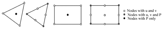
Figure 1 The triangular and quadrilateral elements used for finite element model.

The second-order derivative of f or in other words Hessian matrix f is shown in Equation (18).

$$H=\left[\begin{array}{cccc}\frac{{\mathrm{\partial }}^{2}f}{\mathrm{\partial }{x}_1^2}& {\displaystyle \frac{{\mathrm{\partial }}^{2}f}{\mathrm{\partial }{x}_1\mathrm{\partial }{x}_2}}& \cdots & {\displaystyle \frac{{\mathrm{\partial }}^{2}f}{\mathrm{\partial }{x}_1\mathrm{\partial }{x}_p}}\\ {\displaystyle \frac{{\mathrm{\partial }}^{2}f}{\mathrm{\partial }{x}_2\mathrm{\partial }{x}_1}}& {\displaystyle \frac{{\mathrm{\partial }}^{2}f}{\mathrm{\partial }{x}_2^2}}& \cdots & {\displaystyle \frac{{\mathrm{\partial }}^{2}f}{\mathrm{\partial }{x}_2\mathrm{\partial }{x}_p}}\\ ⋮& ⋮& \ddots & ⋮\\ {\displaystyle \frac{{\mathrm{\partial }}^{2}f}{\mathrm{\partial }{x}_p\mathrm{\partial }{x}_1}}& {\displaystyle \frac{{\mathrm{\partial }}^{2}f}{\mathrm{\partial }{x}_p\mathrm{\partial }{x}_2}}& \cdots & {\displaystyle \frac{{\mathrm{\partial }}^{2}f}{\mathrm{\partial }{x}_p^2}}\end{array}\right]$$

(18)

4.1 The Finite Difference Method

Finite difference method can be considered as a commonly used method in order to accurately estimate the derivatives of a function. The finite difference approximation for derivatives may be obtained by removing negligible terms from the extended Taylor series of function f(x). The first and second order derivatives formulas for the single-objective function areas follows:

$$\frac{df}{dx}\approx \frac{f(x+h)-f(x-h)}{2h}+O(h^2)$$

(19)

$$\frac{d^{2}f}{d{x}^2}\approx \frac{f(x+h)-2f(x)+f(x-h)}{h^2}+O(h^2)$$

(20)

The second order derivatives formulas for the multi-objective function for obtaining Hessian matrix are as follows (for function with two dependent variables for sample):

$$\frac{{\mathrm{\partial }}^{2}f}{\mathrm{\partial }{x}^2}(x,y)\approx \frac{f(x+h,y)-2f(x,y)+f(x-h,y)}{h^2}+O(h^2)$$

(21)

$$\frac{{\mathrm{\partial }}^{2}f}{\mathrm{\partial }{y}^2}(x,y)\approx \frac{f(x,y+h)-2f(x,y)+f(x,y-h)}{h^2}+O(h^2)$$

(22)

$$\begin{gathered} \frac{{\mathrm{\partial }}^{2}f}{\mathrm{\partial }x\mathrm{\partial }y}(x,y)\approx \frac{f(x+h,y+h)-2f(x,y)+f(x-h,y-h)}{2h^2} \\ -\frac{1}{2}(\frac{{\mathrm{\partial }}^{2}f}{\mathrm{\partial }{x}^2}+\frac{{\mathrm{\partial }}^{2}f}{\mathrm{\partial }{y}^2})+O(h^2) \end{gathered}$$

(23)

One of the features of the finite difference approximation is that the simulator calculations of f(x) can be regarded as the black box and it is necessary to perform it only for a selected set of points. Theoretically, the accuracy of the approximation is dependent on the truncation error. This means that the approximation error can be arbitrarily reduced when the steps size is chosen small enough. In practice, due to the limitation in the accuracy of the calculations (rounding error), the accuracy of the approximation is strongly dependent on the step size h.

The truncation error is resulted from omitting the Taylor series terms. On the other hand, the rounding error can be considered as the difference between the numerical value of the function and its actual value. In order to ensure the accuracy of the derivatives approximation, the combined error (truncation error and rounding error) should be minimized. This leads to the well-known problem of step size. Initially, we need to choose a step size that minimizes the truncation error. However, the step size should not be chosen so small which leads to the error of losing the significant figures. It has been shown that as the step size decreases, the approximation error is also reduced. However, as the step size reaches to a critical point, the approximation error starts to increase again.

4.2 The Complex Variable Method

The complex variable method is a numerical differentiation method which is conceptually similar to the finite difference method. However, this method has significant advantages in comparison with the finite difference method. In order to describe the complex variable method, the analytical function f(x) with the scalar complex variable x is considered. The function f(x) can be expanded around the real point x using the Taylor series as follows:

$$f(x+ih)=f(x)+ih\frac{df}{dx}-\frac{h^2}{2!}\frac{d^{2}f}{d{x}^2}-\frac{i{h}^3}{3!}\frac{d^{3}f}{d{x}^3}+\cdots$$

(24)

where $i=\sqrt{-1}$. Hence, this method is also called the approximation with a complex step. The real and imaginary parts of Equation (24) can be considered as follows:

$$\mathrm{\Re }[f(x+ih)]=f(x)-\frac{h^2}{2!}\frac{d^{2}f}{d{x}^2}+O(h^4)$$

(25)

$$\mathrm{\Im }[f(x+ih)]=h\frac{df}{dx}-\frac{h^3}{3!}\frac{d^{3}f}{d{x}^3}+O(h^5)$$

(26)

Dividing Equation (26) by h, the first-order derivative of the function f is obtained as follows:

$$\frac{df}{dx}=\frac{\mathrm{\Im }\left[f(x+ih)\right]}{h}+O\left(h^2\right)$$

(27)

Equation (27) provides an estimation of the first-order derivative of the function f(x) with O(h²). Contrary to the finite difference method, error related to the loss of significant figures is not present in the upper approximation of the first-order derivative, since subtraction is not involved. This can be regarded as the most important advantage of the complex variable approximation method with respect to the finite difference one since the problem of choosing the appropriate step size has been effectively solved. In theory, it is quite possible to choose arbitrarily a small step size, h, without losing the accuracy of the calculations.

It is worth noting that Equation (25) is used for obtaining the approximation of the second-order derivative as follows:

$$\frac{d^{2}f}{d{x}^2}=\frac{2(f(x)-\mathrm{\Re }[f(x+ih)])}{h^2}+O(h^2)$$

(28)

Contrary to the first-order derivative approximation, Equation (28) is associated with the subtraction operator and therefore its accuracy is dependent on the step size h.

The first and second order derivatives formulas for the multi-objective function as follows:

$$\frac{{\mathrm{\partial }}^{2}f}{\mathrm{\partial }{x}^2}(x,y)=\frac{2(f(x,y)-\mathrm{\Re }[f(x+ih,y)])}{h^2}+O(h^2)$$

(29)

$$\frac{{\mathrm{\partial }}^{2}f}{\mathrm{\partial }{y}^2}(x,y)=\frac{2(f(x,y)-\mathrm{\Re }[f(x,y+ih)])}{h^2}+O(h^2)$$

(30)

$$\begin{gathered} \frac{{\mathrm{\partial }}^{2}f}{\mathrm{\partial }x\mathrm{\partial }y}(x,y)=\frac{f(x,y)-\mathrm{\Re }[f(x+ih,y+ih)]}{h^2} \\ -\frac{1}{2}(\frac{{\mathrm{\partial }}^{2}f}{\mathrm{\partial }{x}^2}+\frac{{\mathrm{\partial }}^{2}f}{\mathrm{\partial }{y}^2})+O\left(h^2\right) \end{gathered}$$

(31)

5 The Extended Complex Variable Method

Lai and Crassidis [17] developed a more accurate formula for determining the first and the second-order sensitivities. However, this formulation has not be used in engineering applications yet. The complex unit vector for different angles (15-degree interval) is shown in Figure 2. Using common relations of complex algebra, we can rewrite these vectors in the form of i(p/q) = e^iθ, with a phase angle of θ = (p/q)90 = (p/2q)π. The Taylor series expansion with two complex steps having a phase angle difference of π, can be written as follows:

$$f(x+e^{i\theta }h)=f(x)+\sum _{n=1}^{\mathrm{\infty }}{e}^{ni\theta }\frac{h^n}{n!}{f}^{(n)}(x)$$

(32)

$$f(x+e^{i(\theta +\pi )}h)=f(x)+\sum _{n=1}^{\mathrm{\infty }}{e}^{ni(\theta +\pi )}\frac{h^n}{n!}{f}^{(n)}(x)$$

(33)

It should be noted that e^i(θ±π) = −e^iθ. In addition, instead of presenting the complex step i in power or exponential form, it can be also described by the Euler’s formula e^iθ = cosθ + i sin θ in the trigonometry form. Adding and subtracting of Equations (32) and (33), the following relations are derived:

$$\begin{array}{c}f(x+e^{i\theta }h)+f(x+e^{i(\theta +\pi )}h)\hfill \\ =2f(x)+2\sum _{n=1}^{\mathrm{\infty }}[\cos 2n\theta +i\sin 2n\theta ]\frac{h^{2n}}{(2n)!}{f}^{(2n)}(x)\hfill \end{array}$$

(34)

$$\begin{array}{c}f(x+e^{i\theta }h)-f(x+e^{i(\theta +\pi )}h)\hfill \\ =2\sum _{n=1}^{\mathrm{\infty }}[\cos (2n-1)\theta +i\sin (2n-1)\theta ]\frac{h^{2n-1}}{(2n-1)!}{f}^{(2n-1)}(x)\hfill \end{array}$$

(35)

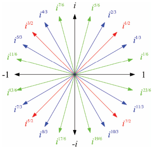
Figure 2 Various complex numbers.

In order to achieve a higher efficiency, we only consider the imaginary part in this case, therefore:

$$\begin{gathered} \mathrm{\Im }(f(x+e^{i\theta }h)+f(x+e^{i(\theta +\pi )}h)) \\ =2\sum _{n=1}^{\mathrm{\infty }}\sin 2n\theta \frac{h^{2n}}{(2n)!}{f}^{(2n)}(x) \end{gathered}$$

(36)

$$\begin{gathered} \mathrm{\Im }(f(x+e^{i\theta }h)-f(x+e^{i(\theta +\pi )}h)) \\ =2\sum _{n=1}^{\mathrm{\infty }}\sin (2n-1)\theta \frac{h^{2n-1}}{(2n-1)!}{f}^{(2n-1)}(x) \end{gathered}$$

(37)

The first and second-order derivatives are obtained for each angle with a complex step using Equations (36) and (37). However, an appropriate angle θ should be chosen to take the advantage of the complex variables method. Considering Equations (36) and (37), one can find the situations where some of the sin functions are zero. These situations are desirable and can be employed to increase the convergence rate of the Taylor series approximation. By choosing appropriate angles, one can reach to the effective and accurate relations. The angles of θ = 45° and θ = 60° are two special angles that vanishes many coefficients of Equations (36) and (37) when they are substituted in the mentioned equations.

5.1 The Case θ = 45°

Substituting θ = 45° in Equation (36), we obtain the following relation:

$$f^{″}(x)=\frac{\mathrm{\Im }[f(x+i^{1/2}h)+f(x+i^{5/2}h)]}{h^2}{E}_{trunc}(h)=\frac{h^4}{360}{f}^{(6)}(x)$$

(38)

Note that when n = 2, the imaginary components are zero sin 2nθ = 0. Therefore, the first non-zero value occurs when n = 3, which corresponds to O(h⁴). Subtraction error is still present in this approximation. However, its truncation error is h⁴f⁽⁶⁾(x)/360, while the corresponding error for Equation (28) is h² f⁽⁴⁾(x)/12.

In order to calculate the first and second-order derivatives using Equations (27) and (38), it is required to determine f(x + ih), f(x + i^1/2h) and f(x + i^5/2h). To obtain the first-order derivative using f(x + i^1/2h) and f(x + i^5/2h), the value θ = 45° is substituted in Equation (37) and the following relation is yielded:

$$f^{\prime }(x)=\frac{\mathrm{\Im }[f(x+i^{1/2}h)-f(x+i^{5/2}h)]}{h\sqrt{2}}{E}_{trunc}(h)=-\frac{h^2}{6}{f}^{(3)}(x)$$

(39)

It should be noted that the error of above equation is equal to that of Equation (27) and therefore similar results are obtained. However, Equation (39) utilizes the same functions as in Equation (38). Since f(x + i^1/2h) − f(x + i^5/2h) = f(x + i^1/2h) − f(x − i^1/2h), the subtraction error is not presented in Equation (39) and the imaginary parts are added with each other. The interesting point in Equations (38) and (39) is that the first and second derivatives are obtained by two times simulation and the accuracy of the second-order sensitivity is in order of fourth.

The first and second order derivatives formulas for the multi-objective function as follows:

$$\frac{{\mathrm{\partial }}^{2}f}{\mathrm{\partial }{x}^2}(x,y)=\frac{\mathrm{\Im }[f(x+i^{1/2}h,y)+f(x+i^{5/2}h,y)]}{h^2}+O(h^4)$$

(40)

$$\frac{{\mathrm{\partial }}^{2}f}{\mathrm{\partial }{y}^2}(x,y)=\frac{\mathrm{\Im }[f(x,y+i^{1/2}h)+f(x,y+i^{5/2}h)]}{h^2}+O(h^4)$$

(41)

$$\begin{gathered} \frac{{\mathrm{\partial }}^{2}f}{\mathrm{\partial }x\mathrm{\partial }y}(x,y)=\frac{\mathrm{\Im }[f(x+i^{1/2}h,y+i^{1/2}h)+f(x+i^{5/2}h,y+i^{5/2}h)]}{2h^2} \\ -\frac{1}{2}(\frac{{\mathrm{\partial }}^{2}f}{\mathrm{\partial }{x}^2}+\frac{{\mathrm{\partial }}^{2}f}{\mathrm{\partial }{y}^2})+O(h^4) \end{gathered}$$

(42)

5.2 The Case θ = 60°

Substituting θ = 60° in Equations (36) and (37), we obtain the following relations:

$$f^{\prime }(x)=\frac{\mathrm{\Im }[f(x+i^{2/3}h)-f(x+i^{8/3}h)]}{h\sqrt{3}}{E}_{trunc}(h)=\frac{h^4}{120}{f}^{(5)}(x)$$

(43)

$$f^{″}(x)=\frac{\mathrm{\Im }[f(x+i^{2/3}h)+f(x+i^{8/3}h)]}{h\sqrt{3}}{E}_{trunc}(h)=\frac{h^2}{24}{f}^{(4)}(x)$$

(44)

As it can be seen, the relation related to the first-order derivative is more accurate than the second-order one. Unlike the second-order derivatives which contain subtraction and truncation errors, the first-order derivatives are not associated with subtraction errors. Therefore, the relations obtained for the case θ = 45°, i.e. Equations (38) and (39), are more suitable for calculating the derivatives.

6 Numerical Examples

For applying the complex variable method, a simulation code is required such that it does not utilize the complex variables. To take the advantage of the method, an automated approach may be used to generate the modified code which can provide both the values of the function and its derivatives. The process of generating the complex version of the original code is as follows:

1. Substituting all real variables with complex ones.
2. Defining all functions and operators that have not been defined for the complex numbers.
3. Using the complex domain for each independent variable and derivative calculation.

The implementation of the FEM code and sensitivities algorithm is done in MATLAB software therefore the first step can be easily conducted since this software accepts complex numbers as standard input data. The MATLAB solver is used to solve the system of equations obtained by finite element discretization. Careful attention should be paid to the second step since the approximation of the complex step is based on the assumption that f(x) is an analytical function. It is absolutely vital to check carefully the validation of this theory when substituting the functions and operators into the complex form. The third step can also be conducted using the obtained relations.

In this section, the extended complex variables method is first validated using an artificial solution. The derivation process is performed on an artificial solution and its result, which is an exact expression, is used for sensitivity calculations. Afterwards, the method is applied for a uniform flow around a cylinder and the results are compared with those of the finite difference method.

6.1 Verification

A velocity field for constructing an artificial solution with steady state, incompressible and laminar assumption is assumed as follows:

$$\begin{array}{rl}\mathbf{u}& =\left\{\begin{array}{c}{v}_x\\ v_y\end{array}\right\}=\left\{\begin{array}{c}\sin (ay)\\ \sin (bx)\end{array}\right\}\\ P& =x\end{array}$$

(45)

Using above relation, the continuity conditions is satisfied and the flow divergence is zero. These relations are substituted in the Navier-Stokes equations to define the body force f ensuring that the momentum equation (Equation (1)) are satisfied. The body forces are obtained as follows:

$$\begin{array}{rl}\mathbf{f}& =\rho \mathbf{u}\cdot \mathrm{\nabla }\mathbf{u}-\mathrm{\nabla }\cdot [2\mu \gamma (\mathbf{u})]+\mathrm{\nabla }P\\ & =\left\{\begin{array}{c}\rho a\sin (bx)\cos (ay)+\mu a^2\sin (ay)+1\\ \rho b\sin (ay)\cos (bx)+\mu b^2\sin (by)\end{array}\right\}\end{array}$$

(46)

The computational domain is square with ten units in length, which is shown in Figure 3. The boundary conditions for the FEM solution are obtained by replacing the coordinates of the boundaries in the Equation (45). One unit for “μ, ρ, b” and two units for “a” are considered. Equations (27), (28), (38) and (39) are used to calculate the sensitivities based on the complex variables method. The sensitivities are computed with respect to the parameter “a” at the point (x, y) = (2, 2). Figure 4 compares the streamlines obtained by the exact and numerical methods. As it can be seen, there is a good agreement between two obtained solutions. Figure 5 shows that the relative error calculated for the velocity and pressure of the flow decreases when the elements number increases. Figure 6 illustrates the relative errors obtained for the first and second order sensitivities of the flow horizontal velocity u with respect to the elements number. The extended complex variable method (ECVM) is applied for calculating the sensitivities. It is observed that there is a one-to-one correspondence between the horizontal velocity error and its sensitivities. It means that the sensitivity error is low when the velocity error is low. Figure 7 compares the first and the second order sensitivities obtained by the ECVM and traditional complex variable method. As it can be seen, the ECVM has the ability of calculating the first and the second order sensitivities with high precision. In Figure 8 the effect of step size on the sensitivity relative error is examined by considering 6728 elements for the problem. As it is expected, both of traditional and extended complex variable methods have almost the same treatment for the first-order sensitivity. However, for the second order sensitivity, they show different behavior with respect to the step size especially for the smaller ones. As it can be seen, the relative error obtained by the extended complex variable method almost remains constant and is independent of step size. Therefore, the ECVM is more preferred for obtaining the second order sensitivity.

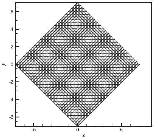
Figure 3 Computational domain and mesh for the validation problem (3200 element).

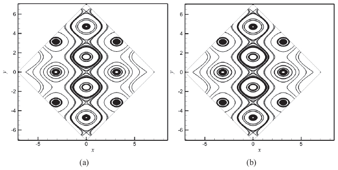
Figure 4 Streamline for the validation problem, (a) exact solution, (b) numerical solution.

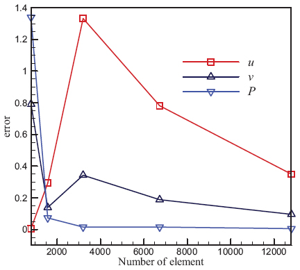
Figure 5 Convergence of velocities and pressure with respect to the number of elements for the validation problem.

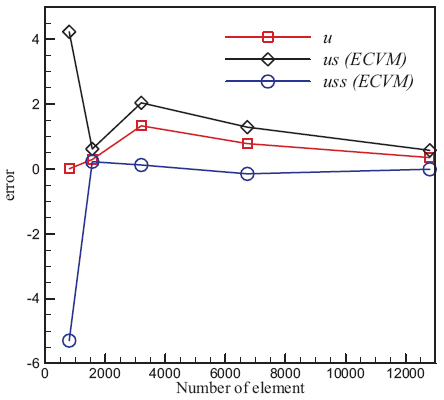
Figure 6 Convergence of the flow horizontal velocity, the first and second-order sensitivity with respect to the number of elements in the validation problem (u: horizontal velocity, us: first-order sensitivity and uss: second-order sensitivity).

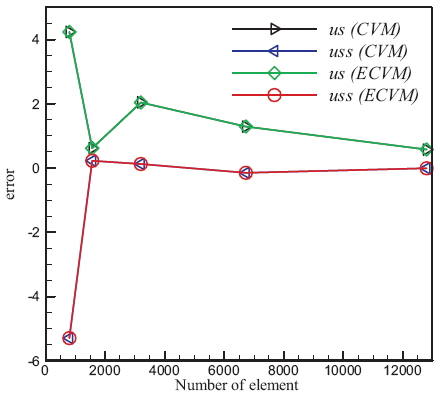
Figure 7 Comparison of solution and convergence of first and second-order sensitivity with respect to the number of elements using the traditional and extended complex variable methods (CVM: traditional complex variable method, ECVM: extended complex variable method).

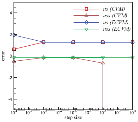
Figure 8 Comparison of convergence of first and second-order sensitivity with respect to the step size using the traditional and extended complex variable methods (CVM: traditional complex variable method and ECVM: extended complex variable method).

6.2 The Flow Around a Cylinder with a Low Reynolds Number

To examine the extended complex variable method in an engineering problem, two-dimensional flow of an incompressible fluid around a cylinder is considered. For this problem, the sensitivity of the drag coefficient (C_d) of the flow with respect to the input velocity is calculated. The cylinder locates in the finite domain Ω: {−15.5 ≤ x ≤ 30.5, −20.5 ≤ y ≤ 20.5} and its diameter is one unit. The cylinder axis is situated at (x, y) = (0,0). The location of the cylinder and its surrounding flow are depicted in Figure 9. The domain is considered large enough to enforce the free flow boundary condition at its top and bottom to have no substantial effect on the results. The value of the velocity in x direction for the inlet (u₀) and also upper and lower boundaries is assumed to be one. The free-stream velocity, known as u_∞, is considered unit. In the domain, the velocity in y direction is set to zero. The boundary conditions of the outflow are free conditions. The Reynolds numbers is chosen 40 which can be solved as steady state solution. Reynolds number is determined based on the free-stream velocity and cylinder diameter. Figure 10(a) shows the finite element model including 7026 elements. Six-node-triangle and three-node elements are considered for the velocity and pressure, respectively. A close-up view of the elements generated around the cylinder is illustrated in Figure 10(b). The number of degree of freedom is 32177.

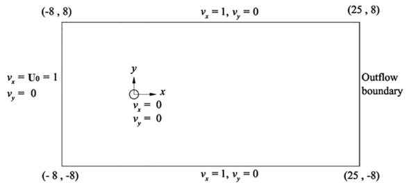
Figure 9 Computational domain and flow boundary conditions around the cylinder.

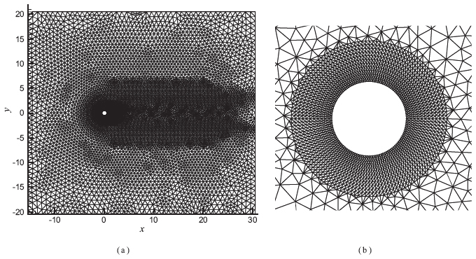
Figure 10 (a) The finit element model for flow pasing around a cylinder, (b) Close-up view of the elements generated around the cylinder.

Figure 11 illustrates the pressure coefficient (C_P) along the cylinder surface for the Reynolds 40. As it can be seen, the results of present finite element model are very close to the experimental values obtained by Grove et al. [19]. In Table 1, the drag coefficients obtained by the present numerical model are compared with those of reported experimentally by Tritton [20]. There is a good agreement between the numerical and experimental results. Figure 12 demonstrates the pressure contours and streamlines obtained by the present numerical model at the behind of the cylinder for Reynolds 40.

To determine the drag sensitivity of the fluid flow with respect to the inlet velocity u₀, Equations (27), (28), (38) and (39) are employed. To achieve this aim, it is required to apply a small perturbation on the value of the inlet velocity. In the complex variables method, the small variation on the inlet velocity is performed as follows:

$$u_0=u_0+i^{n}h$$

(47)

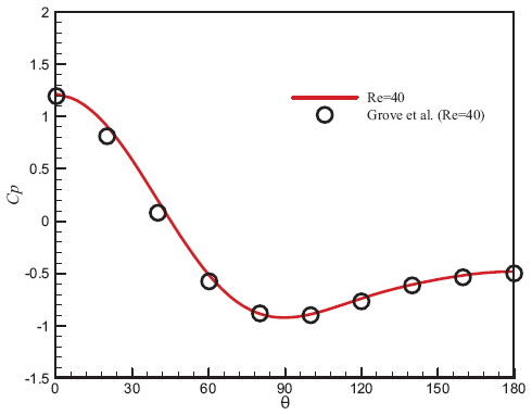
Figure 11 Comparison the pressure coefficients along the cylinder surface CP obtained by the present numerical model and those reported by Grove et al. [19] for Re = 40.

Table 1 Comparison of drag coefficients obtained by the present numerical model and those reported in [20]

Reynolds Number	Present Work	Experimental Results [20]	Relative Error
40	1.5535	1.56	−0.42%

Figure 12 Pressure contours and streamlines resulted from a fluid passing around a cylinder for Re = 40.

In which, h denotes the step and $i=\sqrt{-1}$. Also, the parameter n is equal 1 and 0.5 for the traditional and extended complex variables methods, respectively. The first-order sensitivity of the drag coefficient with respect to the inlet velocity, i.e. $\left(\frac{\mathrm{\partial }{C}_d}{\mathrm{\partial }{u}_0}\right)$, is calculated and presented in Table 2 for various step sizes. In this table, the results of the finite different method achieved using Equation (20) are also reported. The sensitivities calculated by both of the traditional and extended complex variables methods are in good agreement with those of obtained by the finite difference method. As it can be seen, the results of complex variables methods are not sensitive to the step sizes. In other words, the complex variables method leads to accurate and acceptable results for a wide range of step sizes. For larger step sizes, all three mentioned methods provide satisfactory results and are less dependent on the truncation error.

Figures 13 and 14 show the dependency of the drag coefficient and its first-order sensitivity with respect to the number of elements, respectively. They illustrate the dependency of calculated values to the number of elements without any special trend.

Table 2 Comparison of the first-order sensitivity of the drag coefficient with respect to the flow inlet velocity (∂C_d/∂u₀) for Reynolds number 40

Step size	ECVM	CVM	FDM
1.00E-02	2.46016379307537	2.46017884525240	2.46016379244995
1.00E-04	2.46017131841091	2.46017131991619	2.46017131841136
1.00E-06	2.46017131916348	2.46017131916363	2.46017131877440
1.00E-08	2.46017131916355	2.46017131916355	2.46017133331832
1.00E-10	2.46017131916355	2.46017131916356	2.46017317628854
1.00E-12	2.46017131916355	2.46017131916356	2.46003217796442
1.00E-14	2.46017131916355	2.46017131916355	2.45359288442159
1.00E-15	2.46017131916355	2.46017131916355	2.22044604925031
1.00E-16	2.46017131916355	2.46017131916356	1.11022302462515

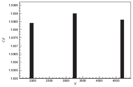
Figure 13 The dependency of the drag coefficient to the number of elements.

The second-order sensitivity of the drag coefficient with respect to the inlet velocity, i.e. $(\frac{{\mathrm{\partial }}^2{C}_d}{\mathrm{\partial }{u}_0^2})$, is calculated and presented in Table 3 for various step sizes. Similar to Table 2, the results of the finite difference method are also reported. According to Table 3, it can be observed that the second-order sensitivities obtained by the traditional complex variables method as well as the finite difference method are dependent to the step size. The results are valid only in the range of 10⁻⁶–10⁻². However, regarding Table 3, it can be seen that the second-order sensitivities obtained by the extended complex variables method remain almost unchanged and are valid for small as well as large step sizes. In other words, the extended complex variable method is accurate for wide range of step size and this can be considered as the main advantage of the method.

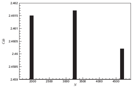
Figure 14 The dependency of the first-order sensitivity of the drag coefficient to the number of elements (Cds : ∂C_d/∂u₀).

Table 3 Comparison of the second-order sensitivity of the drag coefficient with respect to the inlet velocity $({\mathrm{\partial }}^2{C}_d/\mathrm{\partial }{u}_0^2)$ for Reynolds number 40

Step Size	ECVM	CVM	FDM
1.00E-02	1.57062477114552	1.57062020165188	1.57062933445306
1.00E-04	1.57062476960595	1.57062465255819	1.57062489680726
1.00E-06	1.57062476745618	1.56985535681997	1.57185375826429
1.00E-08	1.57062467290612	0.00000000000000	13.32267629550180
1.00E-10	1.57064020735803	−8.88E+04	6.66E+04
1.00E-12	1.57055264253537	−8.88E+08	8.88E+08
1.00E-14	1.67238511906854	−8.88E+12	2.22E+12
1.00E-15	1.77493703674727	−4.44E+14	2.66E+15
1.00E-16	0.00000000000000	−8.88E+16	−2.22E+16

The comparison of Tables 2 and 3 shows that the accuracy of the second-order sensitivity is more affected by the step size. Moreover, the traditional complex variables method used for calculating the second-order sensitivity is somewhat dependent on the step size and the results are affected by the rounding and truncation errors. Hence, the extended complex variables method is suggested as a powerful technique for calculating the first as well as the second order sensitivities and the results are valid for a wide range of step size. Figure 15 illustrates the dependency of the second-order sensitivity of the drag coefficient with respect to the number of elements. By increasing the element number, aconvergence trend is seen for the second-order sensitivity while its effect on the results is negligible.

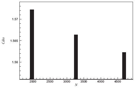
Figure 15 The dependency of the second-order sensitivity of the drag coefficient with respect to the number of elements $(Cdss:{\mathrm{\partial }}^2{C}_d/\mathrm{\partial }{u}_0^2)$.

6.3 The Flow Around Two Rotating Cylinders: Multi-objective Problem

In this example, the sensitivities of a multivariate problem are investigated using various methods. Consider the two-dimensional incompressible fluid flow around the two rotating cylinders with bounded in $\overline{\mathrm{\Omega }}=[0,46]\times [0,41]$. Boundary condition comprises a specific value 1.0 for x velocity component in the inflow. In upper and lower boundaries, the velocity of the y-direction component is zero and boundary conditions of outlet flow are free. The simulation is performed for Re = 40.

Figure 16 illustrates discretizing the geometry around the cylinders via considered parameters for calculating sensitivity analysis. The total number of elements is 5280.

It should be noted that the radius and angular velocity of both left and right cylinders are 0.5 and 5, respectively. The distance between the two cylinders is 2.

The values of drag coefficients sensitivity with respect to the radiuses of cylinders, the distance between the two cylinders and inlet velocities using various approaches are mentioned in Tables 4 and 5. As can be seen from the given tables, the results have a proper similarity.

It is observed that the highest absolute value of the first-order sensitivity among the parameters is the left cylindrical radius. Afterward, the radius of the right cylinder, the inlet velocity, and the distance between the two cylinders respectively have the most impact. However, for second-order sensitivity, the highest absolute value belongs to the radius of the right cylinder, and then the radius of the left cylinder, the distance between the two cylinders and the inlet radius respectively have the most impact. There are also interactions between different parameters.

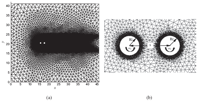
Figure 16 Computational domain and mesh for flow past over two circular cylinder. (a) Computational mesh. (b) Close-up view of the geometric discretization around the circular cylinders.

Table 4 Comparison of the first-order sensitivity of the drag coefficient relative to the various parameter for flow past over two cylindrical cylinders

	ECVM	CVM	FDM
∂CD/∂U0	4.0226	4.0226	4.0226
∂CD/∂Rl	−7.3697	−7.3697	−7.3697
∂CD/∂Rr	−5.7449	−5.7449	−5.7449
∂CD/∂s	0.67737	0.67737	0.67737

Table 5 Comparison of the second-order sensitivity of the drag coefficient relative to the various parameter for flow past over two cylindrical cylinders

	ECVM	CVM	FDM
${\mathrm{\partial }}^2{C}_D/\mathrm{\partial }{U}_0^{2\phantom{{}^0}}$	−4.2389	−4.2388	−4.2389
${\mathrm{\partial }}^2{C}_D/\mathrm{\partial }{R}_l^2$	−120.96450	−120.9650	−120.9656
${\mathrm{\partial }}^2{C}_D/\mathrm{\partial }{R}_r^2$	−123.0995	−123.0995	−123.0993
∂2CD/∂s2	−10.6255	−10.6255	−10.6253
∂2CD/∂U0∂Rl	10.0658	10.0657	10.0658
∂2CD/∂U0∂Rr	27.8215	27.8215	27.8215
∂2Cd/∂U0∂s	−4.8855	−4.8855	−4.8854
∂2CD/∂Rl∂Rr	9.4336	9.4336	9.4336
∂2CD/∂Rl∂s	9.7955	9.7955	9.7956
∂2CD/∂Rr∂s	11.2570	11.2570	11.2569

As can be seen, the Hessian matrix of the function can be calculated for design and optimization purposes with the various methods mentioned with different precision.

7 Conclusion

In this paper, the extended complex variables method was employed to calculate the first and the second order sensitivities of design parameters in an incompressible laminar flow around a cylinder. The finite element method was utilized for modeling the problem. The obtained results were compared with those of achieved by the traditional complex variables method as well as the finite difference method. The results are summarized as follows:

• The flow regime can be accurately modeled using the finite element method.
• The sensitivity analysis is dependent on the step size as well as the number of elements.
• For calculating the first-order sensitivity, the traditional and the extended complex variables methods are independent of step size and lead to highly accurate results. The finite difference method from the step 10⁻¹⁴ to 10⁻² and the others from the step smaller than 10⁻² are unlimitedly reached to the correct answer.
• In comparison with the first-order sensitivity, the second-order sensitivity is more influenced by the step size.
• For calculating the second-order sensitivity, the extended complex variables method results in accurate results for a wide range of step size. By decreasing the step size from 10⁻² to 10⁻¹², the results remain accurate. However, for the traditional complex variables and the finite difference methods, the accuracy remains only up to the step size 10⁻⁶ and the error increases by decreasing the step size.
• The use of complex variables method is recommended when the aim is merely to determine the first-order sensitivity since this method is highly accurate and the step size is not an issue here. However, if additionally the calculation of second-order sensitivity is required, it is preferable to utilize extended complex variables method, since using only two times modeling with the complex variable, the first and second-order sensitivities can be obtained accurately.
• The extended complex variables method is proposed as an appropriate technique for sensitivity analysis which can be effectively utilized in engineering problems. The first and the second order sensitivities obtained by this method are highly accurate and are independent of step size.

Acknowledgements

The author was funded by the Islamic Azad University (IAU). He, therefore, acknowledge with thanks IAU, specially Gorgan Branch.

References

[1] T. T. M. Ta, V. C. Le, and H. T. Pham, Shape optimization for Stokes flows using sensitivity analysis and finite element method, Applied Numerical Mathematics, Vol. 126, pp. 160–179, 2018. https://www.sciencedirect.com/science/article/abs/pii/S0168927417302593

[2] F. Ballarin, A. Manzoni, G. Rozza, and S. Salsa, Shape optimization by free-form deformation: existence results and numerical solution for Stokes flows, Journal of Scientific Computing, 60(3), 537–563, 2014. https://link.springer.com/article/10.1007/s10915-013-9807-8

[3] J. Lambert and L. Gosselin, Sensitivity analysis of heat exchanger design to uncertainties of correlations, Applied Thermal Engineering, Vol. 136, pp. 531–540, 2018. https://www.sciencedirect.com/science/article/abs/pii/S1359431117348925

[4] I. S. Kavvadias, E. M. Papoutsis-Kiachagias, and K. C. Giannakoglou, On the proper treatment of grid sensitivities in continuous adjoint methods for shape optimization, Journal of Computational Physics, Vol. 301, pp. 1–18, 2015. https://www.sciencedirect.com/science/article/pii/S0021999115005318

[5] G. Hu and T. Kozlowski, Application of continuous adjoint method to steady-state two-phase flow simulations, Annals of Nuclear Energy, Vol. 117, pp. 202–212, 2018. https://www.sciencedirect.com/science/article/pii/S0306454918301464

[6] G. Liu, M. Geier, Z. Liu, M. Krafczyk, and T. Chen, Discrete adjoint sensitivity analysis for fluid flow topology optimization based on the generalized lattice Boltzmann method, Computers & Mathematics with Applications, Vol. 68, No. 10, pp. 1374–1392, 2014. https://www.scienc edirect.com/science/article/pii/S0898122114004507

[7] Z. Ding, L. Li, X. Li, and J. Kong, A comparative study of design sensitivity analysis based on adjoint variable method for transient response of non-viscously damped systems, Mechanical Systems and Signal Processing, Vol. 110, pp. 390–411, 2018. https://www.sciencedirect.com/science/article/abs/pii/S0888327018301626

[8] M. Jafari and M. Jafari, Thermal stress analysis of orthotropic plate containing a rectangular hole using complex variable method, European Journal of Mechanics – A/Solids, Vol. 73, pp. 212–223, 2019. https://www.sciencedirect.com/science/article/pii/S0997753817308008

[9] W. K. Anderson, J. C. Newman, D. L. Whitfield, and E. J. Nielsen, Sensitivity analysis forNavier-Stokes equations on unstructured meshes using complex variables, AIAA Journal, Vol. 39(1), pp. 56–63, 2001. https://arc.aiaa.org/doi/abs/10.2514/2.1270

[10] J. N. Lyness and C. B. Moler, Numerical differentiation of analytic functions, SIAM Journal on Numerical Analysis, Vol. 4, No. 2, pp. 202–210, 1967. https://epubs.siam.org/doi/abs/10.1137/0704019

[11] J. N. Lyness, Numerical algorithms based on the theory of complex variable, Proceedings of the 1967 22nd National Conference, ACM, pp. 125–133, 1967. https://dl.acm.org/doi/abs/10.1145/800196.805983

[12] W. Squire and G. Trapp, Using complex variables to estimate derivatives of real functions, SIAM Review, Vol. 40, No. 1, pp. 110–112, 1998. https://epubs.siam.org/doi/abs/10.1137/S003614459631241X

[13] J. R. Martins, P. Sturdza, and J. J. Alonso, The complex-step derivative approximation, ACM Transactions on Mathematical Software (TOMS), Vol. 29, No. 3, pp. 245–262, 2003. https://dl.acm.org/doi/abs/10.1145/838250.838251

[14] J. Martins, I. Kroo, and J. Alonso, An automated method for sensitivity analysis using complex variables, in: 38th Aerospace Sciences Meeting and Exhibit, pp. 689, 2000. https://arc.aiaa.org/doi/abs/10.2514/6.2000-689

[15] D. Rodriguez, A multidisciplinary optimization method for designing inlets using complex variables, in: 8th Symposium on Multidisciplinary Analysis and Optimization, pp. 4875, 2000. https://arc.aiaa.org/doi/abs/10.2514/6.2000-4875

[16] C. Burg and J. Newman III, Computationally efficient, numerically exact design space derivatives via the complex Taylor’s series expansion method, Computers & Fluids, Vol. 32, No. 3, pp. 373–383, 2003. https://www.sciencedirect.com/science/article/abs/pii/S0045793001000445

[17] K.-L. Lai and J. Crassidis, Extensions of the first and second complex-step derivative approximations, Journal of Computational and Applied Mathematics, Vol. 219, No. 1, pp. 276–293, 2008. https://www.sciencedirect.com/science/article/pii/S0377042707004086

[18] J. N. Reddy, 2014, An Introduction to Nonlinear Finite Element Analysis: with applications to heat transfer, fluid mechanics, and solid mechanics, OUP Oxford.

[19] A. S. Grove, F. H. Shair, and E. E. Petersen, An experimental investigation of the steadyseparated flow past a circular cylinder, Journal of Fluid Mechanics, Vol. 19, No. 1, pp. 60–80, 1964. https://www.cambridge.org/core/journals/journal-of-fluid-mechanics/article/an-experimental-investigation-of-the-steady-separated-flow-past-a-circular-cylinder/4C4BBDCFD5E3FD1F80255FCF40998079

[20] D. J. Tritton, “Experiments on the Flow Past a Circular Cylinder at Low Reynolds Numbers,” Journal of Fluid Mechanics, Vol. 6, No. 4, pp. 547–567, 1959. https://www.cambridge.org/core/journals/journal-of-fluid-mechanics/article/experiments-on-the-flow-past-a-circular-cylinder-at-low-reynolds-numbers/0386A4A3A98750248AEB772532863BB6

Biography

Mahdi Hassanzadeh received his M.Sc. Eng. degree in mechanical engineering (solid mechanics) at the Isfahan University of Technology, Iran in 2010. He is currently a Ph.D. student in mechanical engineering at Shahid Beheshti University, Iran. His research focuses on linear and nonlinear finite element method, numerical sensitivity analysis in FEM, optimization and fatigue analysis.

European Journal of Computational Mechanics, Vol. 28_6, 605–634.
doi: 10.13052/ejcm2642-2085.2863
© 2020 River Publishers

Abstract

1 Introduction

2 Navier-Stokes Equations

3 The Pressure-Velocity Finite Element Model

4 Sensitivity Analysis

4.1 The Finite Difference Method

4.2 The Complex Variable Method

5 The Extended Complex Variable Method

5.1 The Case θ = 45°

5.2 The Case θ = 60°

6 Numerical Examples

6.1 Verification

6.2 The Flow Around a Cylinder with a Low Reynolds Number

6.3 The Flow Around Two Rotating Cylinders: Multi-objective Problem

7 Conclusion

Acknowledgements

References

Biography