Pseudospectral Approach to the Shape Optimization of Beams Under Buckling Constraints

Hassan Mohamed Abdelalim Abdalla

Polytechnic Department of Engineering and Architecture, University of Udine, Via delle Scienze 206, 33100 Udine, Italy
E-mail: abdalla.hma@spes.uniud.it

Received 09 May 2022; Accepted 08 September 2022; Publication 14 November 2022

Abstract

In this article, a direct transcription approach to the minimization of the volume of elastic straight beams undergoing plane deformation and subject to buckling loads is presented. In particular, the so-called pseudospectral method is employed, where state variables are approximated by Lagrange interpolating polynomials and static equations are collocated at Legendre-Gauss-Radau nonuniform mesh points. The resulting shape optimization problems are thus transcribed into constrained nonlinear programming problems, which in turn are solved by developed routines. Historical benchmark and academic problems such as simply supported beams subject to a concentrated compressing force, compressed and rotating cantilever beams and simply supported beams under a non-conservative follower distributed load are revisited and numerically solved under the conditions of plane deformation theory. Numerical solutions are discussed and compared to those obtained by the shooting method, which is largely employed for these problems, emphasizing how the proposed method could forecast optimal cross sectional area distributions within a unified fashion and without resorting to accurate guesses beforehand.

Keywords: Shape optimization, buckling, pseudospectral method, transcription, orthogonal collocation method.

1 Introduction

Rods, beams, columns and, more generally, thin structures are conceptual abstractions of physical bodies having one or two dimensions much smaller than the third, whose theory is probably one of the most developed parts in structural engineering. There is a large interest in understanding their mechanical behavior as they can model many elements that would be hard to analyze in the context of three-dimensional elasticity theory. In particular, researchers still investigate their static and dynamic behaviors, to the point that new problems can be formulated [1, 2, 3] and intriguing paradoxes are encountered [4, 5, 6].

Historically, the first elaboration of a theory of beams dates back to Euler, who mimicked the deformed configuration of the beam by a single curve representing the beam axis, introduced certain parameters recording the material orientation relative to that curve and identified vector fields defined on it, called directors, intended to model the principal directions of the beam cross section and to serve as a basis in expressing position vectors on the cross section with respect to a point on the curve [7]. This approach takes the name of the director theory of beams. Later on, several contributions and refined director theories have been introduced by many others, e.g., Kirchhoff and the Cosserat brothers [8].

Parallel to these advancements, an interest has been dedicated to the shape optimization of straight and curved beams under various loads and constraints. Among all, a considerable amount of work addressed the resistance to structural instability, especially against buckling. For instance, the problem of determining the shape of compressed cantilever beam which has the largest Euler buckling load was formulated by Lagrange in 1773. Later on, Clausen proposed a solution for a simply supported beam of circular cross section, yet it did have points where the cross section vanishes, thus inducing infinite stresses in these points; this problem has been overcome by adding a constraint on the minimal value of the cross sectional area, so that given limiting stresses are not exceeded [9]. Since then, many results of structural optimization in the realm of beam theory have been addressed under different load and boundary conditions. Just to list a few, the shape optimization of simply supported and multi-supported beams has been numerically addressed in [10]. The shape optimization of a compressed and twisted column against spatial buckling has been recently revisited in [11], where closed-form expressions for the optimal cross sectional area distributions were derived. The topology optimization of continuum structures under stability requirements has been addressed in [12, 13]. The shape optimization problem of compressed rotating beams has been considered in [14], whereas those concerning with beams on elastic foundations can be found in [15, 16]. Last but not least, other problems have been stated when applied loads are nonconservative, e.g., [17], and when Eringen’s nonlocal elasticity hypothesis is taken into account, e.g., [18, 19].

As far as necessary conditions for optimal solutions are concerned, Pontryagin’s Principle and results from calculus of variations have been considerably recalled. By defining the so-called states, adjoint variables and the Hamiltonian function in a proper way, necessary conditions for extremal solutions can be obtained. Because of their strong coupling, situations in which optimal solutions are derived in closed-form are encountered rarely and the use of numerical integration methods results mandatory.

The overwhelming majority of the aforementioned numerical studies use the so-called indirect methods, where optimal solutions are found by solving the necessary conditions described by a system of nonlinear first-order differential equations that satisfy endpoint conditions. The most well-known strategy pertaining to this method is the so-called shooting method, in which solutions are guessed at endpoints where boundary conditions are not given. The boundary value problem then is forward (or backward) integrated as an initial value problem, where a check is made whether the corresponding boundary values are satisfied. If so, a solution is found, otherwise the initial guesses are adjusted. Despite of its simplicity, errors associated with unknown boundary conditions may considerably amplify as governing equations are integrated, thus requiring sufficiently good guesses of the unknown optimal states and adjoint variables. Conversely, the so-called direct methods have been gaining increasing interest and their theoretical development is more and more refined. Among these methods, the so-called pseudospectral method (or orthogonal collocation method) has been increasing in popularity. This method permits the parameterization of the states and the objective function using specified functional forms. In particular, states are approximated using global polynomials, while governing equations are collocated using nodes obtained from quadrature points. Infinite dimensional functional optimization problems are thus equivalently transcribed into finite dimensional nonlinear programming (NLP) problems.

Pseudospectral methods have been employed by considering many types of collocation point sets and polynomial approximation basis functions. As far as collocation points are concerned, a considerable amount of work has been developed by using Legendre-Gauss, Legendre-Gauss-Lobatto, Legendre-Gauss-Radau and flipped Legendre-Gauss-Radau points (see e.g., [20, 21, 22]). All the aforementioned sets of points are distributed more densely towards the edges of the computation interval and therefore preferably employed for their ability to progressively reduce Runge’s phenomenon. On the other hand, as far as the approximation of the state and/or the objective function is concerned, many attempts have been made available employing Chebyshev polynomials [23], Bernstein polynomials [24], radial basis functions [25] and, more frequently, Lagrange polynomials [26, 27], as these latter satisfy the isolation property.

In this article, and motivated by the conclusions made in [28], a multistage pseudospectral approach to the shape optimization of elastic straight beams undergoing plane deformation is presented, where collocation points are given by Legendre-Gauss-Radau (LGR) points and states are approximated by Lagrange interpolating functions. More specifically, it is desired to show that the resulting functional optimization problems can be addressed within a single framework, thus hinting that numerical optimal solutions could be forecast within a unified fashion and bypassing the numerical issues related to the shooting method, commonly employed in the literature. The article is organized as follows: Governing equations for plane deformation (Euler-Bernoulli’s theory) and generalized plane deformation (including extensibility and shear measures) referring to a linearly elastic and homogeneous material are firstly presented and optimal necessary conditions are recalled in Section 2. Section 3 illustrates the corresponding LGR transcription procedure in its multistage form. Eventually, three academic shape optimization examples are numerically solved and discussed in Section 4 and conclusions are drawn in Section 5.

2 Theoretical Framework

Consider a beam of a given length $L$ and made of a material exhibiting a linear stress–strain relation. The beam axis is represented by a plane curve in a rectangular Cartesian coordinate system, whose horizontal and vertical axes are denoted by $\overline{z}$ and $\overline{y}$, respectively. Let $\mathbf{i}$ and $\mathbf{j}$ be the unit vectors along $\overline{z}$ and $\overline{y}$, respectively, and $\mathbf{k}=\mathbf{i}\times \mathbf{j}$. The beam axis coincides with the centroidal line of the beam cross section. Suppose that the bending rigidity of the beam and the angle between the tangent to the beam axis and the $\overline{z}$ axis are denoted by $EI$ and $\theta$, respectively, both functions of the arc length $S\in [0,L]$ measured from one end point, namely $EI(S)$ and $\theta (S)$. Denoting by $A(S)$ the area of the cross section at the generic curvilinear coordinate $S$, the material volume of the beam is given by

$$W={\int }_0^{L}A(S)\mathit{d}S.$$

(1)

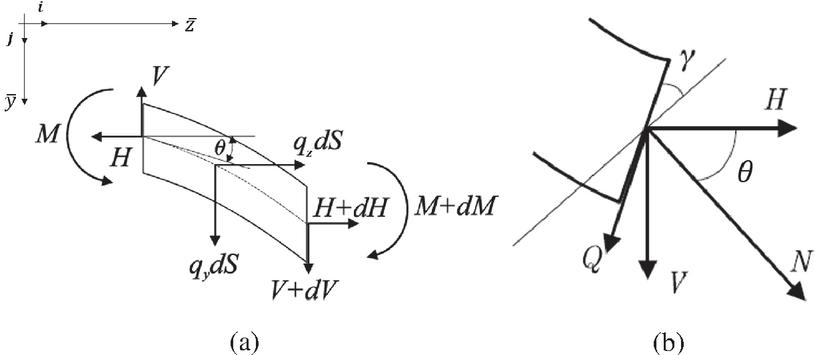
Let $q_z(S)$ and $q_y(S)$ denote the intensities of the distributed forces at $S$ along $\overline{z}$ and $\overline{y}$, respectively, both per unit of the beam axis (see Figure 1a). Moreover, let $H(S)$ and $V(S)$ denote the components of the internal force $\mathbf{R}(S)$ and $\mathbf{\text{M}}(S)$ denote the internal couple at an arbitrary section of the beam of coordinate $S$, which represent the influence of the cut-off part $[0,S)$ of the beam on the element of length $dS$. Hence, $\mathbf{R}(S)=H(S)\mathbf{i}+V(S)\mathbf{j}$, and $\mathbf{M}(S)=M(S)\mathbf{k}$.

Figure 1 Coordinate system, load configuration and definition of the employed variables for (a) plane deformation and (b) generalized plane deformation.

2.1 Governing Equations for Plane Deformation

Based on the framework reported in [29], if Euler-Bernoulli assumptions hold, namely plane sections in the natural state remain plane in the deformed state and extensional and shear rigidity are infinite, the nonlinear governing equations for the static behavior of an elastic beam are¹

$$\{\begin{array}{cc}\frac{dH}{dS}=-q_z,\hfill & \\ \frac{dV}{dS}=-q_y,\hfill & \\ \frac{dM}{dS}=-V\cos \theta +H\sin \theta ,\hfill & \\ \frac{dz}{dS}=\cos \theta ,\hfill & \\ \frac{dy}{dS}=\sin \theta ,\hfill & \\ \frac{d\theta }{dS}=M/(E\eta A^{\sigma }),\hfill & \end{array}$$

(2)

where $E$ is Young’s modulus and $\eta$ and $\sigma$ are two constants depending on the shape of the cross section (for a circular cross section, $\eta =1/4\pi$ and $\sigma =2$).

2.2 Governing Equations for Generalized Plane Deformation

In case the extensibility of the beam axis $\epsilon$ and the rotation of the cross section with shear angle $\gamma$ are taken into account (Figure 1b), the variation of coordinates along $S$ take the form [29]

$$\{\begin{array}{cc}\frac{dz}{dS}=(1+\epsilon )\cos \theta ,\hfill & \\ \frac{dy}{dS}=(1+\epsilon )\sin \theta ,\hfill & \end{array}$$

(3)

and the internal couple is given by

$$M=EI\left(\frac{d\theta }{dS}-\frac{d\gamma }{dS}\right).$$

(4)

Moreover, referring to the constitutive equations of the beam in the form that follows from [30], the shear angle and the rod axis extensibility take the form (see Figure 1b)

$$\{\begin{array}{cc}\sin \gamma =\frac{cQ}{GA},\hfill & \\ \epsilon =\frac{N}{EA},\hfill & \end{array}$$

(5)

where $c$ is the shear correction factor, $EA$ and $GA$ are the extensional and shear rigidity, respectively, while $Q$ and $N$ are the components of the internal force in the direction of the sheared plane and tangent to the beam axis, respectively, which according to Engesser’s model, are given by [30]

$$\{\begin{array}{cc}N=H\frac{\cos (\theta -\gamma )}{\cos \gamma }+V\frac{\sin (\theta -\gamma )}{\cos \gamma },\hfill & \\ Q=V\frac{\cos \theta }{\cos \gamma }-H\frac{\sin \theta }{\cos \gamma }.\hfill & \end{array}$$

(6)

2.3 Problem Formulation and Necessary Conditions

With prescribed loads $q_z$ and $q_y$, cross sectional distribution $A$ and boundary conditions at endpoints, the static equations aims at assessing the static behavior of the beam by determining the horizontal $H$ and vertical $V$ internal forces, the internal couple $M$, coordinates $z$ and $y$ and the angle $\theta$ along the beam axis. As a consequence, these latter variables may be referred to as the state variables of the problem. Here, we are interested in finding out the cross sectional area distribution so that the beam is as light as possible, while static equations are satisfied. In other words, we define the lightest beam under a given load as the beam having the shape that any other beam of the same length and smaller volume buckles. More precisely, denoting by $\mathbf{x}\in \mathcal{𝒳}$ the state variables and recasting static equations into the form

$$\frac{d\mathbf{x}}{dS}=\mathbf{f}(S,\mathbf{x},A),$$

(7)

where $\mathbf{f}:[0,L]\times \mathcal{𝒳}\times \mathcal{𝒜}\to \mathcal{𝒳}$, the shape optimization problem associated with a goal functional $J(\mathbf{x},A)$ and characterized by states at endpoints ${\mathbf{\text{x}}}_0$ and ${\mathbf{\text{x}}}_L$, an admissible state space $\mathcal{𝒳}$ and an admissible shape space $\mathcal{𝒜}$ consists in finding the cross sectional area distribution $A:[0,L]\to \mathcal{𝒜}$ which minimizes $J$ and such that, if $\mathbf{x}(0)={\mathbf{\text{x}}}_0$, then $\mathbf{x}(S)\in \mathcal{𝒳}$ for all $S\in [0,L]$ and $\mathbf{x}(L)={\mathbf{\text{x}}}_L$.

Denoting by $n$, $b$ and $q$ the number of elastic states, boundary conditions and path constraints, respectively, and letting $\mathcal{𝒳}$ be ${ℝ}^n$, $\mathcal{𝒜}$ be ${ℝ}^{+}$ and referring to the set of boundary conditions and inequality constraints by $\mathit{\varphi }:{ℝ}^n\times {ℝ}^n\to {ℝ}^b$ and $\mathbf{c}:[0,L]\times {ℝ}^n\times ℝ\to {ℝ}^q$, respectively, the aforementioned shape optimization problem may be generally recast as follows:

Problem 1

$\underset{A(S)}{\min }$	$J=\mathcal{ℳ}(\mathbf{x}(0),\mathbf{x}(L))+{\displaystyle {\int }_0^L}\mathcal{ℒ}(S,\mathbf{x},A)\mathit{d}S,$	(8)
t.	${\displaystyle \frac{d\mathbf{x}}{dS}}=\mathbf{f}(S,\mathbf{x},A),$
	$\mathit{\varphi }(\mathbf{x}(0),\mathbf{x}(L))=\mathbf{0},$
	$\mathbf{c}(S,\mathbf{x},A)\le \mathbf{0}.$

Here, $\mathcal{ℳ}:{ℝ}^n\times {ℝ}^n\to ℝ$ takes the name of Mayer term and represents a punctual term at either $S=0$ or $S=L$, or both. The integral term whose integrand is $\mathcal{ℒ}:[0,L]\times {ℝ}^n\times ℝ\to ℝ$ is called the Lagrange term and it is a distributed cost associated with the whole domain $S\in [0,L]$.

First-order necessary conditions for extremal solutions of Problem 1 can be determined from the application of variational principles in calculus of variations. These conditions are typically derived by defining the following augmented Hamiltonian function

$$\mathcal{\mathscr{H}}(S,\mathbf{x},\mathbf{p},\mathit{\mu },A)=\mathcal{ℒ}+{\mathbf{p}}^{\top }\mathbf{f}-{\mathit{\mu }}^{\top }\mathbf{c},$$

(9)

where $\mathbf{p}:[0,L]\to {ℝ}^n$ is the vector containing the costate or adjoint variables and $\mathit{\mu }:[0,L]\to {ℝ}^q$ is the vector of Lagrange multipliers associated with the inequality constraints $\mathbf{c}$. In particular, first-order optimality conditions are given by [31]

$$\frac{d\mathbf{x}}{dS}={\left[\frac{\partial \mathcal{\mathscr{H}}}{\partial \mathbf{p}}\right]}^{\top },$$	(10)
$$\frac{d\mathbf{p}}{dS}=-{\left[\frac{\partial \mathcal{\mathscr{H}}}{\partial \mathbf{x}}\right]}^T,$$	(11)
$$A^{*}=\arg \underset{A\in \mathcal{𝒜}}{\min }\mathcal{\mathscr{H}},$$	(12)
$$\mathit{\varphi }(\mathbf{x}(0),\mathbf{x}(L))=\mathbf{0},$$	(13)
$$\mathbf{p}(0)=-\frac{\partial \mathcal{ℳ}}{\partial \mathbf{x}(0)}+{\mathit{\nu }}^T\frac{\partial \mathit{\varphi }}{\partial \mathbf{x}(0)},$$	(14)
$$\mathbf{p}(L)=\frac{\partial \mathcal{ℳ}}{\partial \mathbf{x}(L)}-{\mathit{\nu }}^T\frac{\partial \mathit{\varphi }}{\partial \mathbf{x}(L)},$$	(15)
$$\mathcal{\mathscr{H}}(0)=\mathcal{\mathscr{H}}(L)=0,$$	(16)
$${\mu }_j=0,\text{when}{c}_j(S,\mathbf{x},A)<0,j=1,\mathrm{\dots },q$$	(17)
$${\mu }_j\le 0,\text{when}{c}_j(S,\mathbf{x},A)=0,j=1,\mathrm{\dots },q$$	(18)

where $\mathit{\nu }\in {ℝ}^b$ is the Lagrange multiplier vector associated with boundary conditions $\mathit{\varphi }$. Because Equations (10) and (11) arise from differentiation of a Hamiltoninan function, they form a Hamiltonian system. Equation (12) is known as Pontryagin’s Principle which, in case $A^{*}$ lies on the interior of $\mathcal{𝒜}$, may be expressed as

$$\frac{\partial \mathcal{\mathscr{H}}}{\partial A}=0.$$

(19)

Finally, boundary conditions on the costate variables (14) and (15) are called transversality conditions, while the conditions on the Lagrange multipliers of the inequality constraints $\mathbf{c}$ are referred to as complementary slackness conditions. Equations (10)–(18) form a Hamiltonian boundary-value problem, whose solution is called an extremal and consists of the state, costate and any Lagrange multipliers that satisfy boundary conditions and any interior point constraints on the state and costate. Due to the strong coupling between states, costates and the objective function, closed form solutions are rarely encountered, thus hindering one to resort to numerical methods.

3 LGR Transcription Procedure

In this section, the transcription procedure of Problem 1 into a constrained NLP is described. The fundamental steps of such transcription consist of the domain discretization into multiple mesh intervals and the continuous-to-discrete conversion of states and controls.

As a preliminary remark, and without loss of generality, the numerical framework is developed with respect to a pseudo domain $\xi \in [-1,1]$ to which the finite interval $S\in [0,L]$ can be mapped by the linear transformation

$$\{\begin{array}{cc}S=\frac{L}{2}\xi +\frac{L}{2},\hfill & \\ \xi =\frac{2}{L}S-1.\hfill & \end{array}$$

(20)

Problem 1 is then formulated in terms of the variable $\xi$ as follows.

Problem 2

$\underset{A(\xi )}{\min }$	$J=\mathcal{ℳ}(\mathbf{x}(-1),\mathbf{x}(1))+{\displaystyle \frac{L}{2}}{\displaystyle {\int }_{-1}^1}\mathcal{ℒ}(\xi ,\mathbf{x}(\xi ),A(\xi ))\mathit{d}\xi ,$	(21)
t.	${\displaystyle \frac{d\mathbf{x}(\xi )}{d\xi }}={\displaystyle \frac{L}{2}}\mathbf{f}(\xi ,\mathbf{x}(\xi ),A(\xi )),$
	$\mathit{\varphi }(\mathbf{x}(-1),\mathbf{x}(1))=\mathbf{0},$
	$\mathbf{c}(\xi ,\mathbf{x}(\xi ),A(\xi ))\le \mathbf{0}.$

Suppose now that the interval $\xi \in [-1,1]$ is divided into a mesh consisting of $K$ mesh intervals $[{\xi }_{k-1},{\xi }_k]$, $k=1,2,\mathrm{\dots },K$, where $({\xi }_0,{\xi }_1,\mathrm{\dots },{\xi }_K)$ are the mesh points, which have the property $-1={\xi }_0<{\xi }_1<\mathrm{\cdots }<{\xi }_K=1$. Next, let ${\mathbf{x}}^{(k)}(\xi )$ and $A^{(k)}(\xi )$ be the vector containing states and the objective function in the mesh interval $k$. Thus, the objective functional can be recast as

$J$	$=\mathcal{ℳ}({\mathbf{x}}^{(1)}(-1),{\mathbf{x}}^{(K)}(1))$
	$\mathrm{\hspace{1em}}+{\displaystyle \frac{L}{2}}{\displaystyle \sum _{k=1}^K}{\displaystyle {\int }_{{\xi }_{k-1}}^{{\xi }_k}}\mathcal{ℒ}(\xi ,{\mathbf{x}}^{(k)}(\xi ),A^{(k)}(\xi ))\mathit{d}\xi .$	(22)

Moreover, the differential constraint and the path constraints in mesh interval $k$ can be written as

$$\frac{d{\mathbf{x}}^{(k)}(\xi )}{d\xi }=\frac{L}{2}\mathbf{f}(\xi ,{\mathbf{x}}^{(k)}(\xi ),A^{(k)}(\xi ))$$

(23)

and

$$\mathbf{c}(\xi ,{\mathbf{x}}^{(k)}(\xi ),A^{(k)}(\xi ))\le \mathbf{0},$$

(24)

respectively, whereas the boundary conditions may be recast as

$$\mathit{\varphi }({\mathbf{x}}^{(1)}(-1),{\mathbf{x}}^{(K)}(1))=\mathbf{0}.$$

(25)

Because the state must be continuous at each interior mesh point, it is required that the condition $\mathbf{x}({\xi }_k^{-})=\mathbf{x}({\xi }_k^{+})$ be satisfied at $({\xi }_1,{\xi }_2,\mathrm{\dots },{\xi }_{K-1})$. Using the LGR pseudospectral scheme, this continuity condition across mesh points is easy to implement. In particular, the state in each mesh interval $k=1,2,\mathrm{\dots },K$ is approximated as

$${\mathbf{x}}^{(k)}(\xi )\approx {\mathbf{X}}^{(k)}(\xi )=\sum _{j=1}^{N_k+1}{\mathbf{X}}_j^{(k)}{\mathrm{\ell }}_j^{(k)}(\xi ),$$

(26)

where ${\mathbf{X}}_j^{(k)}$ ($j=1,2,\mathrm{\dots },N_k$) are the approximations of the state functions at the $N_k$ LGR points in mesh interval $k$ and

$${\mathrm{\ell }}_j^{(k)}(\xi )=\prod _{l=1,l\ne j}^{N_k+1}\frac{\xi -{\xi }_l^{(k)}}{{\xi }_j^{(k)}-{\xi }_l^{(k)}},$$

where $({\xi }_1^{(k)},{\xi }_2^{(k)},\mathrm{\dots },{\xi }_{N_k}^{(k)})$ are the LGR collocation points in mesh interval $k$ defined on the sub-interval $\xi \in [{\xi }_{k-1},{\xi }_k]$. The LGR collocation points in mesh interval $k$ are given by the roots of the polynomial $P_{N_k-1}(\xi )+P_{N_k}(\xi )$, where $P_{N_k-1}$ and $P_{N_k}$ are the Legendre polynomials of degree $N_k-1$ and $N_k$, respectively. It is worth noting that the point ${\xi }_{N_k+1}^{(k)}$ is a noncollocated point. Differentiating (26) with respect to $\xi$, one obtains

$$\frac{d{\mathbf{X}}^{(k)}(\xi )}{d\xi }=\sum _{j=1}^{N_k+1}{\mathbf{X}}_j^{(k)}\frac{d{\mathrm{\ell }}_j^{(k)}(\xi )}{d\xi }.$$

(27)

Besides, the cost functional of Equation (22) is approximated using a multiple interval LGR quadrature as

$$J=\mathcal{ℳ}({\mathbf{X}}_1^{(1)},{\mathbf{X}}_{N_K+1}^{(K)})+\frac{L}{2}\sum _{k=1}^K\sum _{j=1}^{N_k}{\omega }_j^{(k)}\mathcal{ℒ}({\xi }_j^{(k)},{\mathbf{X}}_j^{(k)},A_j^{(k)}),$$

(28)

where ${\mathbf{X}}_1^{(1)}$ and ${\mathbf{X}}_{N_K+1}^{(K)}$ are the approximations of $\mathbf{x}({\xi }_0=-1)$ and $\mathbf{x}({\xi }_K=1)$, respectively, ${\omega }_j^{(k)}$ ($j=1,2,\mathrm{\dots },N_k$) are the LGR quadrature weights in mesh interval $k$, given by

$$\{\begin{array}{cc}{\omega }_1^{(k)}=\frac{2}{N_k^2},\hfill & \\ {\omega }_i^{(k)}=\frac{1}{(1-{\xi }_i^{(k)}){\left[\frac{d{P}_{N_k-1}(\xi )}{d\xi }\right]}_{{\xi }_i^{(k)}}^2},(i=2,3,\mathrm{\dots },N_k)\hfill & \end{array}$$

(29)

and $A_j^{(k)}$ ($j=1,2,\mathrm{\dots },N_k$) are the approximations of the objective function at the $N_k$ LGR points in mesh interval $k$. Collocating the differential constraints of Equation (23) at the $N_k$ LGR points by means of (27), one obtains

$$\sum _{j=1}^{N_k+1}{D}_{ij}^{(k)}{\mathbf{X}}_j^{(k)}-\frac{L}{2}\mathbf{f}({\xi }_i^{(k)},{\mathbf{X}}_i^{(k)},A_i^{(k)})=\mathbf{0},i=1,2,\mathrm{\dots },N_k,$$

(30)

where

$$D_{ij}^{(k)}={\left[\frac{d{\mathrm{\ell }}_j^{(k)}(\xi )}{d\xi }\right]}_{{\xi }_i^{(k)}},i=1,\mathrm{\dots },N_k,j=1,\mathrm{\dots },N_k+1,k=1,\mathrm{\dots },K,$$

(31)

is the $N_k\times (N_k+1)$ differentiation matrix in mesh interval $k$.

Next, the path constraint of Equation (24) in the mesh interval $k$ are enforced at the $N_k$ LGR points as

$$\mathbf{c}({\xi }_i^{(k)},{\mathbf{X}}_i^{(k)},A_i^{(k)})\le \mathbf{0},i=1,2,\mathrm{\dots },N_k.$$

(32)

Furthermore, the boundary conditions of Equation (25) are approximated as

$$\mathit{\varphi }({\mathbf{X}}_1^{(1)},{\mathbf{X}}_{N_K+1}^{(K)})=\mathbf{0}.$$

(33)

It is noted that the continuity in the state at the interior mesh points is enforced via the condition

$${\mathbf{X}}_{N_k+1}^{(k)}={\mathbf{X}}_1^{(k+1)},k=1,2,\mathrm{\dots },K-1.$$

(34)

However, it is worth noting that this constraint is taken into account explicitly and therefore the NLP that arises from the LGR pseudospectral approximation is then to minimize the cost function of Equation (28) subject to the algebraic constraints (30)–(33).

Introducing the notation

$${\mathit{\xi }}^{(k)}=\left[\begin{array}{c}\hfill {\xi }_1^{(k)}\hfill \\ \hfill {\xi }_2^{(k)}\hfill \\ \hfill \mathrm{⋮}\hfill \\ \hfill {\xi }_{N_k}^{(k)}\hfill \end{array}\right],{\mathbf{X}}^{(k)}=\left[\begin{array}{c}\hfill {\mathbf{X}}_1^{(k)}\hfill \\ \hfill {\mathbf{X}}_2^{(k)}\hfill \\ \hfill \mathrm{⋮}\hfill \\ \hfill {\mathbf{X}}_{N_k}^{(k)}\hfill \end{array}\right],k=1,2,\mathrm{\dots },K-1,$$

$${\mathit{\xi }}^{(K)}=\left[\begin{array}{c}\hfill {\xi }_1^{(K)}\hfill \\ \hfill {\xi }_2^{(K)}\hfill \\ \hfill \mathrm{⋮}\hfill \\ \hfill {\xi }_{N_K+1}^{(K)}\hfill \end{array}\right],{\mathbf{X}}^{(K)}=\left[\begin{array}{c}\hfill {\mathbf{X}}_1^{(K)}\hfill \\ \hfill {\mathbf{X}}_2^{(K)}\hfill \\ \hfill \mathrm{⋮}\hfill \\ \hfill {\mathbf{X}}_{N_K+1}^{(K)}\hfill \end{array}\right],$$

$${\mathbf{A}}^{(k)}=\left[\begin{array}{c}\hfill A_1^{(k)}\hfill \\ \hfill A_2^{(k)}\hfill \\ \hfill \mathrm{⋮}\hfill \\ \hfill A_{N_k}^{(k)}\hfill \end{array}\right],{\mathit{\omega }}^{(k)}=\left[\begin{array}{c}\hfill {\omega }_1^{(k)}\hfill \\ \hfill {\omega }_2^{(k)}\hfill \\ \hfill \mathrm{⋮}\hfill \\ \hfill {\omega }_{N_k}^{(k)}\hfill \end{array}\right],{\mathbf{L}}^{(k)}=\left[\begin{array}{c}\hfill \mathcal{ℒ}({\xi }_1^{(k)},{\mathbf{X}}_1^{(k)},A_1^{(k)})\hfill \\ \hfill \mathcal{ℒ}({\xi }_2^{(k)},{\mathbf{X}}_2^{(k)},A_2^{(k)})\hfill \\ \hfill \mathrm{⋮}\hfill \\ \hfill \mathcal{ℒ}({\xi }_{N_k}^{(k)},{\mathbf{X}}_{N_k}^{(k)},A_{N_k}^{(k)})\hfill \end{array}\right],$$

$${\mathbf{f}}^{(k)}=\left[\begin{array}{c}\hfill \mathbf{f}({\xi }_1^{(k)},{\mathbf{X}}_1^{(k)},A_1^{(k)})\hfill \\ \hfill \mathbf{f}({\xi }_2^{(k)},{\mathbf{X}}_2^{(k)},A_2^{(k)})\hfill \\ \hfill \mathrm{⋮}\hfill \\ \hfill \mathbf{f}({\xi }_{N_k}^{(k)},{\mathbf{X}}_{N_k}^{(k)},A_{N_k}^{(k)})\hfill \end{array}\right],{\mathbf{C}}^{(k)}=\left[\begin{array}{c}\hfill \mathbf{c}({\xi }_1^{(k)},{\mathbf{X}}_1^{(k)},A_1^{(k)})\hfill \\ \hfill \mathbf{c}({\xi }_2^{(k)},{\mathbf{X}}_2^{(k)},A_2^{(k)})\hfill \\ \hfill \mathrm{⋮}\hfill \\ \hfill \mathbf{c}({\xi }_{N_k}^{(k)},{\mathbf{X}}_{N_k}^{(k)},A_{N_k}^{(k)})\hfill \end{array}\right],$$

$$k=1,2,\mathrm{\dots },K$$

and letting

$$\mathit{\xi }=\left[\begin{array}{c}\hfill {\mathit{\xi }}^{(1)}\hfill \\ \hfill {\mathit{\xi }}^{(2)}\hfill \\ \hfill \mathrm{⋮}\hfill \\ \hfill {\mathit{\xi }}^{(K)}\hfill \end{array}\right]\in {ℝ}^{N+1},\mathit{\omega }=\left[\begin{array}{c}\hfill {\mathit{\omega }}^{(1)}\hfill \\ \hfill {\mathit{\omega }}^{(2)}\hfill \\ \hfill \mathrm{⋮}\hfill \\ \hfill {\mathit{\omega }}^{(K)}\hfill \end{array}\right]\in {ℝ}^N,$$

$$\mathbf{X}=\left[\begin{array}{c}\hfill {\mathbf{X}}^{(1)}\hfill \\ \hfill {\mathbf{X}}^{(2)}\hfill \\ \hfill \mathrm{⋮}\hfill \\ \hfill {\mathbf{X}}^{(K)}\hfill \end{array}\right]\in {ℝ}^{(N+1)\times n},\mathbf{A}=\left[\begin{array}{c}\hfill {\mathbf{A}}^{(1)}\hfill \\ \hfill {\mathbf{A}}^{(2)}\hfill \\ \hfill \mathrm{⋮}\hfill \\ \hfill {\mathbf{A}}^{(K)}\hfill \end{array}\right]\in {ℝ}^N,$$

$$\mathbf{L}=\left[\begin{array}{c}\hfill {\mathbf{L}}^{(1)}\hfill \\ \hfill {\mathbf{L}}^{(2)}\hfill \\ \hfill \mathrm{⋮}\hfill \\ \hfill {\mathbf{L}}^{(K)}\hfill \end{array}\right]\in {ℝ}^N,\mathbf{F}=\left[\begin{array}{c}\hfill {\mathbf{f}}^{(1)}\hfill \\ \hfill {\mathbf{f}}^{(2)}\hfill \\ \hfill \mathrm{⋮}\hfill \\ \hfill {\mathbf{f}}^{(K)}\hfill \end{array}\right]\in {ℝ}^{N\times n},$$

$$\mathbf{C}=\left[\begin{array}{c}\hfill {\mathbf{C}}^{(1)}\hfill \\ \hfill {\mathbf{C}}^{(2)}\hfill \\ \hfill \mathrm{⋮}\hfill \\ \hfill {\mathbf{C}}^{(K)}\hfill \end{array}\right]\in {ℝ}^{N\times q},$$

where $N={\sum }_{k=1}^K{N}_k$, the cost functional and discretized differential constraints given in Equations (28) and (30) can be written compactly as

$$J=\mathcal{ℳ}({\mathbf{X}}_1,{\mathbf{X}}_{N+1})+\frac{L}{2}{\mathit{\omega }}^{\top }\mathbf{L}$$

(35)

and

$$\mathbf{DX}-\frac{L}{2}\mathbf{F}=\mathbf{0},$$

(36)

where $\mathbf{D}\in {ℝ}^{N\times (N+1)}$ is the LGR differentiation matrix, which has a block structure with nonzero elements defined by the matrix given in Equation (31). The extra column of $\mathbf{D}$ is due to the Lagrange polynomial at the noncollocated point ${\xi }_{N+1}=1$. Finally, the discretized path constraints of Equation (32) and boundary conditions of Equation (33) are expressed as

$$\mathbf{C}\le \mathbf{0}$$

(37)

and

$$\mathit{\varphi }({\mathbf{X}}_1,{\mathbf{X}}_{N+1})=\mathbf{0},$$

(38)

respectively. Hence, Problem 2 may be transcribed into the following discrete NLP problem.

Problem 3

$\underset{\mathbf{X},\mathbf{A}}{\min }$	$J=\mathcal{ℳ}({\mathbf{X}}_1,{\mathbf{X}}_{N+1})+{\displaystyle \frac{L}{2}}{\mathit{\omega }}^{\top }\mathbf{L}$	(39)
t.	$\mathbf{DX}-{\displaystyle \frac{L}{2}}\mathbf{F}=\mathbf{0},$
	$\mathit{\varphi }({\mathbf{X}}_1,{\mathbf{X}}_{N+1})=\mathbf{0},$
	$\mathbf{C}\le \mathbf{0}.$

Problem 3 is a finite-dimensional NLP constrained problem, whose decision variables are the approximation of the states and the objective function at the LGR points. The resulting NLP is suitably reshaped and solved by using dedicated solvers. In this article, Matlab optimization toolbox fmincon has been chosen as the NLP solver. Initial guesses have been set to be linear or constants in the domain for both states and objective function. Numerical solutions have been forecast $j$ times, each one with $N^{<j>}$ mesh points that progressively increases. Denoting the optimal goal functional associated with $N^{<j>}$ by $J^{*}(N^{<j>})$, it was found that $J^{*}(N^{<j+1>})-J^{*}(N^{<j>})\le {10}^{-6}$ for $N^{<j>}\ge 50$.

4 Benchmark Problems

4.1 Lagrange’s Beam

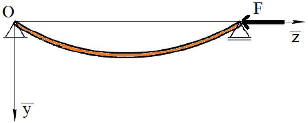
In order to motivate the present approach, Pearson’s formulation of the Lagrange’s beam problem is recalled [32], namely the simply supported beam of circular cross section ($\eta =\frac{1}{4\pi }$ and $\sigma =2$) and maximum resistance to buckling under axial compression (see Figure 2).

Figure 2 Simply supported beam under buckling load.

4.1.1 The plane deformation case

Here, it is implicitly assumed that extensional and shear rigidity are infinite. The nonlinear static equation for this case is [29]

$$\frac{d}{dS}\left(A^2\frac{d\theta }{dS}\right)+\frac{4\pi }{E}F\sin \theta =0.$$

(40)

Introducing the dimensionless quantities $s=\frac{S}{L},a=\frac{A}{L^2},w=\frac{W}{L^3},\lambda =\frac{4\pi F}{E{L}^2}$, Equation (40) reads

$${(a^2{\theta }^{\prime })}^{\prime }+\lambda \sin \theta =0,$$

(41)

where a prime denotes the first derivative with respect to $s$, subject to the boundary conditions

$$\theta (1/2)=0,{\theta }^{\prime }(0)=0.$$

(42)

Due to symmetry considerations, the problem can be considered only for $S\in [0,L/2]$; the normalized half volume of the beam is therefore

$$w={\int }_0^{1/2}a(s)\mathit{d}s.$$

(43)

Introducing $x_1=\theta$, $x_2=a^2{\theta }^{\prime }$, $x_3=w$ and $x_4=\lambda$ as state variables, the beam resistance to buckling under axial compression as a shape optimization problem can be expressed in the following two different ways:

1. To find the distribution of material along the length of the beam so that the beam is of minimum volume and supports a given load $\tilde{\lambda }$ without buckling, i.e.,

$\underset{a(s)}{\min }$	${\displaystyle {\int }_0^{1/2}}a(s)\mathit{d}s$	(44)
s.t.	$x_1^{\prime }=x_2/a^2,$
	$x_2^{\prime }=-\tilde{\lambda }{x}_1,$
	$x_1(1/2)=0,$
	$x_2(0)=0.$

2. To find the distribution of material along the length of the beam of a given half volume $\tilde{w}$ which gives the largest possible buckling load, i.e.,

$\underset{a(s)}{\min }$	$-x_4(1/2)$	(45)
s.t.	$x_1^{\prime }=x_2/a^2,$
	$x_2^{\prime }=-x_1{x}_4,$
	$x_3^{\prime }=a,$
	$x_4^{\prime }=0,$
	$x_1(1/2)=0,$
	$x_2(0)=0,$
	$x_3(0)=0,$
	$x_3(1/2)=\tilde{w}.$

Note that static equations have been linearized in the two versions, since the optimal beam is supposed to still remain straight, i.e., no post-buckling analysis is considered. Moreover, goal functionals are of Lagrange and Mayer types in the first and second problem, respectively. A different form of the two problems above has been considered in [33], where the optimal beam having the same volume of a uniform one has been numerically obtained by means of the shooting method. In [33], Hamiltoninans and necessary conditions for optimal solutions have been firstly derived. By employing the notation described in the present article, they are given by

$$\mathcal{\mathscr{H}}=a+\frac{p_1{x}_2}{a^2}-\tilde{\lambda }{p}_2{x}_1,$$

$$a=\sqrt[3]{2p_1{x}_2},$$

$$p_1^{\prime }=\tilde{\lambda }{p}_2,p_2^{\prime }=-p_1/a^2,$$

$$p_1(0)=p_2(1/2)=0,$$

for the first version and

$$\mathcal{\mathscr{H}}=\frac{p_1{x}_2}{a^2}-p_2{x}_1{x}_4+p_{3}a,$$

$$a=\sqrt[3]{\frac{2p_1{x}_2}{p_3}},$$

$$p_1^{\prime }=p_2{x}_4,p_2^{\prime }=-\frac{p_1}{a^2},p_3^{\prime }=0,p_4^{\prime }=p_2{x}_1$$

$$p_1(0)=p_2(1/2)=p_4(0)=0,p_4(1/2)=-1,$$

for the second version, where $p_k$ are the costates associated with states $x_k$, with $k=1,2,3,4$. It is obvious that the condition $p_1(0)=0$ always implies that the cross section vanishes at the end of the beam, i.e., $a(0)=0$, conveying to Clausen’s solution.

In [33], it has been found that the goal functional associated with the optimal cross sectional area distribution in the first version associated with $\tilde{\lambda }={\pi }^2$ is $w^{*}=0.433$. Once this latter result is introduced into the second version as $\tilde{w}$, one obtains $x_4^{*}(1/2)=9.869\approx {\pi }^2$, underlying the equivalence of the two versions. Nonetheless, this preliminary numerical consideration takes place only if accurate guesses of $p_k$ are provided. For many problems, this condition is not simply guaranteed, as costate variables are not physically interpretable in most of the cases. Conversely, by employing the approach presented in the present article, there is no need to obtain necessary conditions for optimality and therefore, unlike the shooting method, the burden of accurately guessing optimal states and costates is bypassed. In particular, by simply taking

$$\mathbf{f}=[x_2/a^2-\tilde{\lambda }{x}_1]$$

and

$$\mathbf{f}=[x_2/a^2-x_1{x}_{4}a0]$$

for the first and second formulation, respectively, optimal states and optimal objective functions can be directly obtained by solving the corresponding NLP problems.

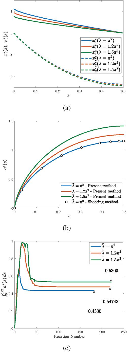
Figure 3 Optimal (a) states and (b) cross sectional area distributions for the first version of Lagrange’s beam problem. (c) The objective functional versus the iterations number.

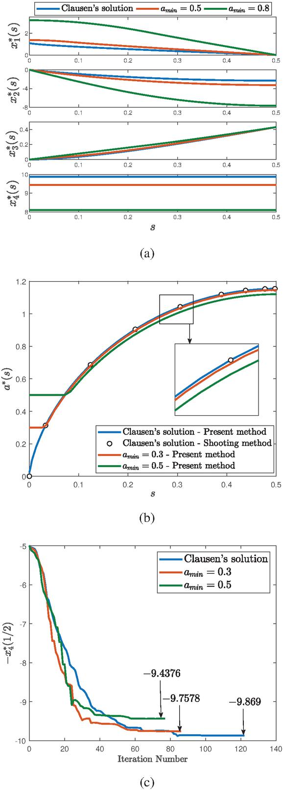
As far as the first formulation is concerned, Figures 3a and 3b show the optimal states and optimal cross sectional area distributions obtained by the method of the present article with $\tilde{\lambda }={\pi }^2,1.2{\pi }^2$ and $1.5{\pi }^2$. As expected, the high $\tilde{\lambda }$, the high the volume required to withstand the load without buckling. Optimal values of the goal functional associated with the first problem are $w^{*}=0.4330$, 0.4743 and 0.5303, respectively. Numerical solution associated with $\tilde{\lambda }={\pi }^2$ has been compared to that obtained in [33]. It is easy to notice that both solutions are in good agreement and the cross section vanishes at the end (Clausen’s solution). In parallel, one may be interested in imposing a minimal value of the cross sectional area distribution $a_{min}$. Unlike the shooting method, the present approach allows to consider this requirement as an inequality constraint. For instance, besides the Clausen’s solution, optimal states as well as optimal area distributions have been numerically forecast so that $a\ge 0.3$ and $a\ge 0.5$ (Figures 4a and 4b). Optimal values for the goal functional associated with the second formulation read $x_4^{*}(1/2)=9.7578,\mathrm{\hspace{0.25em}7.4376}$ for the Clausen’s solution, with $a\ge 0.3$ and with $a\ge 0.5$, respectively, namely the maximum buckling resistance diminishes as the $a_{min}$ increases for a given half volume $\tilde{w}=0.4330$. Finally, Figures 3c and 4c display the evolution of the goal functional in function of the iteration number.

Figure 4 Optimal (a) states and (b) cross sectional area distributions for the second version of Lagrange’s beam problem. (c) The objective functional versus the iterations number.

4.1.2 The generalized plane deformation case

Here, the same load configuration as well as the symmetric buckling mode are considered, but now with finite values for the extensional and shear rigidity. To this purpose, Equations (3)–(6) are employed. When the beam is subject to a compressive force $F$, then $H=-F$ and $V=0$ and therefore the axis extensibility and the shear angle are given by [30]

$$\epsilon =-\frac{F}{EA}\frac{\cos (\theta -\gamma )}{\cos \gamma }$$

(46)

and

$$\gamma =\frac{1}{2}\arcsin \left(\frac{2cF}{GA}\sin \theta \right),$$

(47)

respectively. Now, defining the angle $\alpha =\theta -\gamma$ and taking into consideration the linearized version of the static equations, one obtains

$$\{\begin{array}{cc}{M}^{\prime }=F\frac{1-\frac{F}{EA}}{1-\frac{cF}{GA}}\alpha ,\hfill & \\ {\alpha }^{\prime }=\frac{M}{EI}\hfill & \end{array}$$

(48)

and subject to the boundary conditions

$$M(0)=0,\alpha (1/2)=0.$$

(49)

Introducing the additional dimensionless quantities $m=\frac{4\pi M}{E{L}^3}$, $\tilde{\mu }=\frac{F}{E{L}^2}$ and $\tilde{\beta }=\frac{cF}{G{L}^2}$, the minimum mass shape optimization problem reads

$\underset{a(s)}{\min }$	${\displaystyle {\int }_0^{1/2}}a(s)\mathit{d}s$	(50)
s.t.	$x_1^{\prime }={\displaystyle \frac{x_2}{a^2}},$
	$x_2^{\prime }=-\tilde{\lambda }\left({\displaystyle \frac{a-\tilde{\mu }}{a-\tilde{\beta }}}\right)x_1,$
	$x_1(1/2)=0,$
	$x_2(0)=0,$

where the states $x_1$ and $x_2$ refer to $\alpha$ and $m$, respectively, and $\tilde{\lambda }$, $\tilde{\mu }$ and $\tilde{\beta }$ are linked through the relation

$$\tilde{\lambda }={\pi }^2\frac{1-\tilde{\beta }}{1-\tilde{\mu }}.$$

(51)

In the present notation, necessary conditions for optimal solutions are given by

$$\mathcal{\mathscr{H}}=a+\frac{p_1{x}_2}{a^2}-\tilde{\lambda }\left(\frac{a-\tilde{\mu }}{a-\tilde{\beta }}\right)p_2{x}_1,$$

$$\frac{\partial \mathcal{\mathscr{H}}}{\partial a}=0=1-\frac{2p_1{x}_2}{a^3}-p_2{x}_1\frac{\tilde{\lambda }(\tilde{\mu }-\tilde{\beta })}{{(a-\tilde{\beta })}^2},$$

$$p_1^{\prime }=\tilde{\lambda }\left(\frac{a-\tilde{\mu }}{a-\tilde{\beta }}\right)p_2,p_2^{\prime }=-p_1/a^2,$$

$$p_1(0)=p_2(1/2)=0.$$

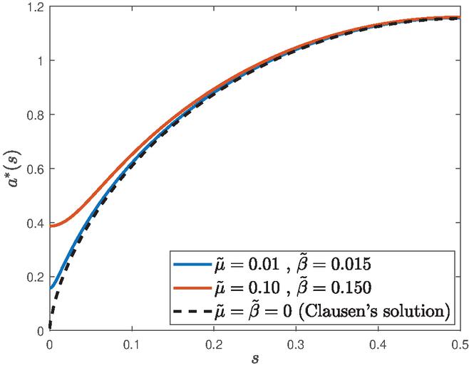
It is worth noting that shear and compressibility have opposite influence on Euler buckling load and for $\tilde{\beta }=\tilde{\mu }=0$, one obtains the classical dimensionless critical load. Besides, according to [34], it is assumed that $\tilde{\mu }<1$ and $\tilde{\beta }>\tilde{\mu }$. Besides, and unlike the plane deformation case, here the cross section does not vanish at the beam end, i.e.,

$$a(0)=\tilde{\beta }+\sqrt{\tilde{\lambda }(\tilde{\mu }-\tilde{\beta })x_1(0)p_2(0)},$$

confirming that the shape of the optimal beam and its end depends on the load and material.

Table 1 Optimal values of the goal functional, the minimal and maximal values of the normalized cross sectional area distributions for different instances of $\tilde{\beta }$ and $\tilde{\mu }$

$\tilde{\beta }$	$\tilde{\mu }$	$\tilde{\lambda }$	${\int }_0^{1/2}{a}^{*}(s)\mathit{d}s$	$a^{*}(0)$	$a^{*}(1/2)$
0	0	9.868	0.4330	0	1.1545
$1.5\times {10}^{-2}$	$1\times {10}^{-3}$	9.731	0.4376	0.1573	1.1580
	$1\times {10}^{-2}$	9.820	0.4350	0.1035	1.1565
$1.5\times {10}^{-1}$	$1\times {10}^{-3}$	8.398	0.4637	0.5104	1.1601
	$1\times {10}^{-2}$	8.474	0.4628	0.5026	1.1603
	$1\times {10}^{-1}$	9.321	0.4504	0.3868	1.1608

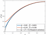
Table 1 lists optimal values of the goal functional and minimal and maximal values of the optimal normalized cross sectional area distribution for different values of $\tilde{\beta }$ and $\tilde{\mu }$. Moreover, optimal cross area distributions for two instances of $\tilde{\beta }$ and $\tilde{\mu }$ are shown in Figure 5 and compared to Clausen’s solution.

Figure 5 Optimal cross sectional area distribution for two instances of $\tilde{\beta }$ and $\tilde{\mu }$ (solid lines) compared to Clausen’s solution (dashed line).

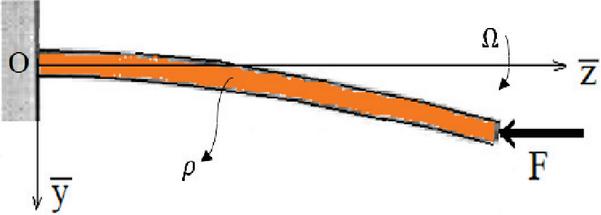
Figure 6 A compressed rotating cantilever beam.

4.2 Compressed and Rotating Cantilever

Consider an elastic cantilevered beam of length $L$ fixed at an end and compressed by a concentrated force having constant intensity $F$ at the other end. Suppose that the beam has a circular cross section ($I=\frac{1}{4\pi }{A}^2$), that its axis is initially straight and always lies on a plane defined by the system $\overline{z}-O-\overline{y}$ and that it rotates with a constant angular velocity $\mathrm{\Omega }$ about its axis (see Figure 6). The volume of the rod is still given by relation (1). It is known that at a certain angular velocity, even when the force $F$ is not acting, the beam loses stability so that it can be bent under the action of centrifugal forces. The problem of determining the critical rotation speed and the post-critical behavior of the beam described has been subject of many investigations, e.g., [35, 36]. The variation of the coordinates as well as the components of the internal force and internal couple along $S$ read

$$\{\begin{array}{cc}\frac{dz}{dS}=\cos \theta ,\hfill & \\ \frac{dy}{dS}=\sin \theta ,\hfill & \\ \frac{dH}{dS}=0,\hfill & \\ \frac{dV}{dS}=-\rho \mathrm{\Omega }y,\hfill & \\ \frac{dM}{dS}=-V\cos \theta +H\sin \theta ,\hfill & \\ \frac{d\theta }{dS}=\frac{4\pi M}{E{A}^2},\hfill & \end{array}$$

(52)

where $\rho$ denotes the line density of the beam. To the system (52), the following boundary conditions are adjoined:

$$z(0)=y(0)=V(L)=M(L)=0,H(L)=-F.$$

(53)

Introducing the dimensionless quantities $s=\frac{S}{L}$, $a=\frac{A}{L^2}$, $\xi =\frac{y}{L}$, $\tilde{w}=\frac{W}{L^3}$, $m=\frac{4\pi M}{E{L}^3}$, $v=\frac{4\pi V}{E{L}^2}$, ${\lambda }_1^2=\frac{4\pi \rho \mathrm{\Omega }{L}^2}{E}$, ${\lambda }_2^2=\frac{4\pi F}{E{L}^2}$ and the new dependent variable $u=-v/{\lambda }_1$, the right-hand side of the linearized static equations may be written as

$$\mathbf{f}=[a{x}_2{\lambda }_1{x}_3{x}_4/a^2{\lambda }_1{x}_1\text{-}{\lambda }_2{x}_3]$$

and subject to

$$x_1(1)=x_2(0)=x_3(0)=x_4(1)=0,$$

(54)

where the states $x_1$, $x_2$, $x_3$ and $x_4$ refer to $u$, $u^{\prime }/a$, $\theta$ and $a^2{\theta }^{\prime }$, respectively, and the prime refers to the first derivative with respect to $s$. Therefore, the minimum mass compressed rotating beam problem reads

$\underset{a(s)}{\min }$	$\tilde{w}={\displaystyle {\int }_0^1}a(s)\mathit{d}s$	(55)
s.t.	$x_1^{\prime }=a{x}_2,$
	$x_2^{\prime }={\lambda }_1{x}_3,$
	$x_3^{\prime }={\displaystyle \frac{x_4}{a^2}},$
	$x_4^{\prime }={\lambda }_1{x}_1-{\lambda }_2{x}_3,$
	$x_1(1)=0,$
	$x_2(0)=0,$
	$x_3(0)=0,$
	$x_4(1)=0.$

The Hamiltonian function and necessary conditions for optimality are given by

$$\mathcal{\mathscr{H}}=a+p_{1}a{x}_2+p_2{\lambda }_1{x}_3+p_3\frac{x_4}{a^2}+p_4({\lambda }_1{x}_1-{\lambda }_2{x}_3),$$

$$a={\left\{\frac{2p_3{x}_4}{1+p_1{x}_2}\right\}}^{1/3},$$

$$p_1^{\prime }=-{\lambda }_1{p}_4,p_2^{\prime }=-p_{1}a,p_3^{\prime }=-{\lambda }_1{p}_2+{\lambda }_2{p}_4,p_4^{\prime }=-\frac{p_3}{a^2},$$

$$p_1(0)=p_2(1)=p_3(1)=p_4(0)=0.$$

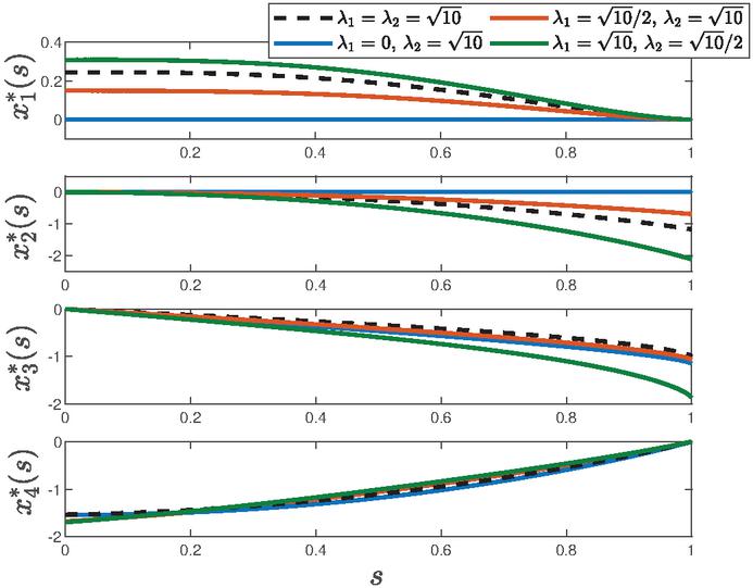
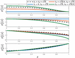
Figure 7 Optimal states for the compressed rotating beam problem with four instances of ${\lambda }_1$ and ${\lambda }_2$.

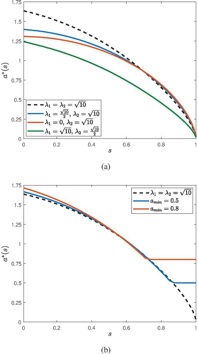
Observations made in [37] by reformulating the optimality system in the canonical formalism can significantly simplify the analysis, leading to a boundary value problem suitably handled by Runge-Kutta methods, yet initial values need to be determined through variational principles. Here, instead, numerical solutions for the optimal states (Figure 7) and optimal cross sectional area distributions (Figure 8a) for different instances of ${\lambda }_1$ and ${\lambda }_2$ have been determined bypassing this step. In agreement with [37], it can be easily seen that the optimal rod is cigar shaped at the top. Optimal values for $\tilde{w}$, $a(0)$ and $a(1)$ are reported in Table 2. Eventually, optimal solutions after imposing a constraint on the minimal value of the cross sectional area distribution ($a_{min}=0.5$ and 0.8) are shown in Figure 8b.

Figure 8 Optimal cross sectional area distributions for the compressed rotating beam problem with (a) four instances of ${\lambda }_1$ and ${\lambda }_2$ and with (b) different values of $a_{min}$.

4.3 Pflüger’s Beam

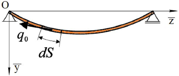
In this section, the optimal cross sectional area distribution for a simply supported beam loaded by a uniformly distributed follower-type nonconservative load of constant intensity $q_0$ is considered, commonly referred to as Pflüger beam in literature (see Figure 9). Here, since the distributed force is tangent to the beam axis, it follows

$$q_z=-q_0\cos \theta ,q_y=-q_0\sin \theta$$

(56)

and therefore the variation of the components of the contact force is given by

$$\frac{dH}{dS}=q_0\cos \theta ,\frac{dV}{dS}=q_0\sin \theta .$$

(57)

After simple algebraic manipulations, the linearized static equations along the normalized coordinate $s=\frac{S}{L}$ reduces to

$$m^{\prime \prime }+\frac{\widehat{\lambda }}{a^2}(1-s)m=0,$$

(58)

where a prime still denotes the derivative with respect to $s$, $m=\frac{4\pi M}{E{L}^3}$, $a=\frac{A}{L^2}$, $\widehat{w}=\frac{W}{L^3}$ and $\widehat{\lambda }=\frac{4\pi q_0}{EL}$ and subject to

$$m(0)=m(1)=0.$$

(59)

Table 2 Optimal values of the goal functional and the minimal and maximal values of the normalized cross sectional area distributions for different instances of ${\lambda }_1$ and ${\lambda }_2$

${\lambda }_1$	${\lambda }_2$	${\tilde{w}}^{*}$	$a^{*}(0)$	$a^{*}(1)$
$\sqrt{10}$	$\sqrt{10}$	1.0848	1.640	0.0393
$\sqrt{10}/2$	$\sqrt{10}$	1.0082	1.398	0.0439
$0$	$\sqrt{10}$	0.9804	1.307	0.0465
$\sqrt{10}$	$\sqrt{10}/2$	0.7948	1.245	0.0267

Figure 9 Pflüger’s simply supported beam under distributed nonconservative follower load.

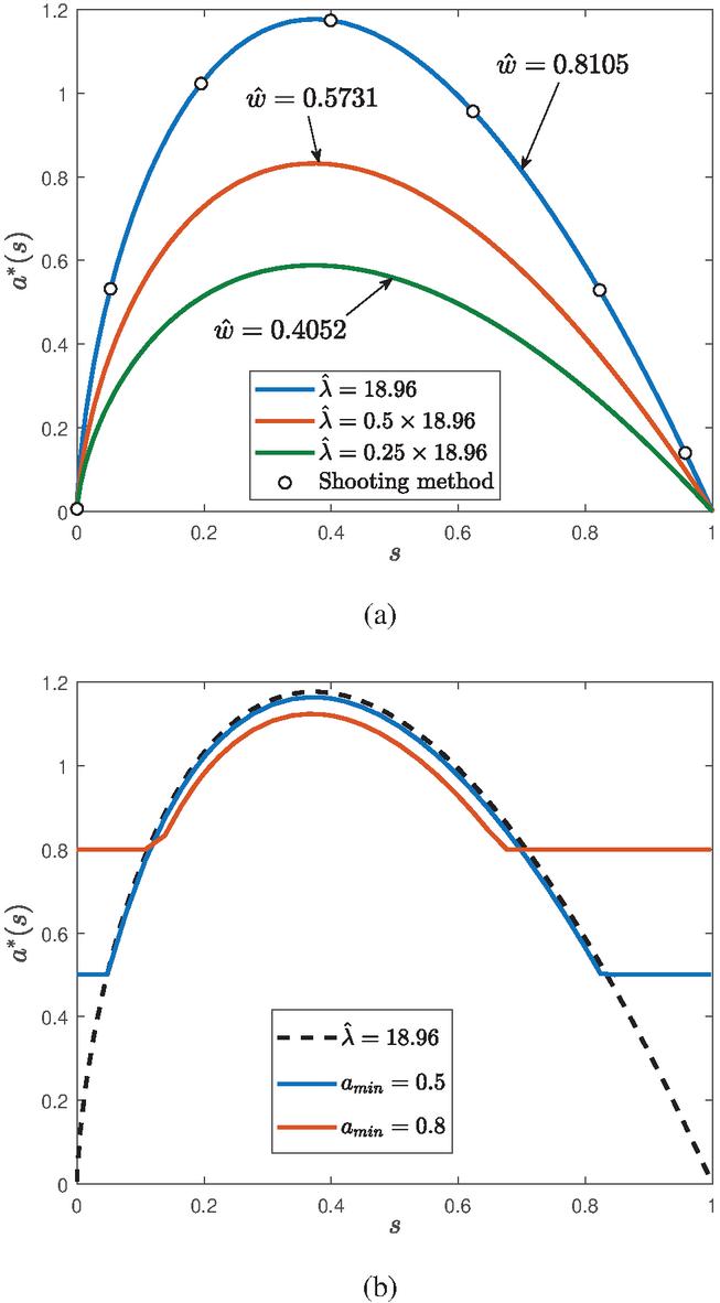
Figure 10 Optimal cross sectional area distributions for the Pflüger’s beam problem with (a) three instances of $\widehat{\lambda }$ and (b) two instances of $a_{min}$.

Introducing the states $x_1=m$ and $x_2=m^{\prime }$, the right-hand side of static equations may be written as

$$\mathbf{f}=[x_2\widehat{\lambda }(s-1)x_1/a^2\mathrm{\hspace{0.25em}1}]$$

and subject to

$$x_1(0)=x_1(1)=0.$$

(60)

Therefore, the minimum mass Pflüger’s beam problem reads

$\underset{a(s)}{\min }$	$\widehat{w}={\displaystyle {\int }_0^1}a(s)\mathit{d}s$	(61)
s.t.	$x_1^{\prime }=x_2,$
	$x_2^{\prime }={\displaystyle \frac{\widehat{\lambda }(s-1)x_1}{a^2}},$
	$x_1(0)=0,$
	$x_1(1)=0.$

The Hamiltonian function and necessary conditions for optimality are given by

$$\mathcal{\mathscr{H}}=a+p_1{x}_2+\widehat{\lambda }\frac{x_1{p}_2}{a^2}(s-1),$$

$$a={\left\{2\widehat{\lambda }{x}_1{p}_2(s-1)\right\}}^{1/3},$$

$$p_1^{\prime }=-\widehat{\lambda }\frac{p_2}{a^2}(s-1),p_2^{\prime }=-p_1,$$

$$p_2(0)=p_2(1)=0.$$

The problem has been solved by using Pontryagin’s Principle in [17]. It is shown that the boundary value problem relevant for determining the optimal distribution of area along the beam axis has simple eigenvalues. The lowest eigenvalue of the beam with constant cross-section having unit volume is 18.956266.

Figures 10a shows optimal cross sectional area distribution for $\widehat{\lambda }=18.96$ by the method of the present article and the comparison with that obtained by the shooting method, showing good agreement. Furthermore, solutions associated with the normalized loads $0.25\widehat{\lambda }$ and $0.5\widehat{\lambda }$ have been also forecast. The corresponding optimal weights are 0.8105, 0.5731 and 0.4052. It is worth noting that the cross area vanishes at both ends and does not achieve its maximum value at $s=0.5$. Eventually, Figure Figure 10b shows the effect of the minimal area constraint $a_{min}$ on the optimal solution.

5 Conclusions

A direct transcription approach to the shape optimization of beams under plane deformation is proposed, where states are approximated by Lagrange interpolating polynomials and static equations are collocated at Legendre-Gauss-Radau mesh points. The shape optimization problem is firstly projected into a pseudospectral domain and then transcribed into a constrained nonlinear programming problem. The shape optimization of three academic problems is then addressed, where numerical solutions are obtained by means of developed Matlab routines and compared to the literature. It is shown that the proposed approach treats these kind of problems within a unified fashion by bypassing guess-related issues associated with numerical techniques commonly employed in literature.

Acknowledgment

The author thanks Prof. Dušan Zorica for the fruitful discussion and useful suggestions on the content and organization of the article.

Footnotes

Hereinafter, the dependence on $S$ is omitted for brevity.

References

[1] Wang, C.Y. (2016) Longest reach of a cantilever with a tip load. European Journal of Physics 37, 012001. doi: https://doi.org/10.1088/0143-0807/37/1/012001

[2] Abdalla, H.M.A. and Casagrande, D. (2020) On the longest reach problem in large deflection elastic rods. International Journal of Non-Linear Mechanics 119, 103310. doi: https://doi.org/10.1016/j.ijnonlinmec.2019.103310

[3] Lewis, W.J., Russell, J.M. and Li, T.Q. (2021) Moment-less arches for reduced stress state. Comparisons with conventional arch forms. Computers and Structures 251, 106524. doi: https://doi.org/10.1016/j.compstruc.2021.106524

[4] Strozzi, A., Bertocchi, E. and Mantovani, S. (2019) A paradox in curved beams. Proceedings of Institution of Mechanical Engineers: Part C 233, pp. 2830–2833. doi: https://doi.org/10.1177/0954406218797980

[5] Abdalla, H.M.A., Casagrande, D. and Strozzi, A. (2020) A unified relaxed approach easing the practical application of a paradox in curved beams. Proceedings of Institution of Mechanical Engineers: Part C 234, pp. 4535–4542. doi: https://doi.org/10.1177/0954406220924693

[6] Bigoni, D., Kirillov, O.N., Misseroni, D., Noselli, G. and Tommasini, M. (2018) Flutter and divergence instability in the Pflüger column: Experimental evidence of the Ziegler destabilization paradox. Journal of the Mechanics and Physics of Solids 116, pp. 99–116. doi: https://doi.org/10.1016/j.jmps.2018.03.024

[7] Antman, S.S. (1973) The theory of rods. In: Truesdell, C. (Eds.), Linear Theories of Elasticity and Thermoelasticity. Springer, Berlin. doi: https://doi.org/10.1007/978-3-662-39776-3\_6

[8] Green, A.E. and Laws, N. (1968) A General Theory of Rods. In: Kröner E. (eds) Mechanics of Generalized Continua. Springer, Berlin, Heidelberg. doi: https://doi.org/10.1098/rspa.1966.0163

[9] Seyranian, A.P. and Privalova, O.G. (2003) The Lagrange problem on an optimal column: old and new results. Structural and Multidisciplinary Optimization 25, pp. 393–410. doi: https://doi.org/10.1007/s00158-003-0333-4

[10] Kirikov, M. and Altus, E. (2011) Functional gradient as a tool for semi-analytical optimization for structural buckling. Computers & Structures 89, pp. 1563–1573. doi: https://doi.org/10.1016/j.compstruc.2011.05.012

[11] Kobelev, V. (2022) Stability optimization for a simultaneously twisted and compressed rod. Multidiscipline Modeling in Materials and Structures 18, pp. 24–42. doi: https://doi.org/10.1108/MMMS-12-2021-0205

[12] Gao, X. and Ma, H. (2015) Topology optimization of continuum structures under buckling constraints. Computers & Structures 157, pp. 142–152. doi: https://doi.org/10.1016/j.compstruc.2015.05.020

[13] Mendes, E., Sivapuram, R., Rodriguez, R., Sampaio, M. and Picelli, R. (2021) Topology optimization for stability problems of submerged structures using the TOBS method. Computers & Structures 259, 106685 doi: https://doi.org/10.1016/j.compstruc.2021.106685

[14] Braun, D.J. (2008) On the optimal shape of compressed rotating rod with shear and extensibility. International Journal of Non-Linear Mechanics 43, pp. 131–139. doi: https://doi.org/10.1016/j.ijnonlinmec.2007.11.001

[15] Novakovic, B.B (2015) Optimal shape of a column with clamped-elastically supported ends positioned on elastic foundation. Theoretical and Applied Mechanics 42, pp. 191–200. doi: https://doi.org/10.2298/TAM1503191N

[16] Banichuk, N., Barsuk, A., Ivanova, S., Makeev, E., Niettaanmaki, P. and Tuovinen, T. (2018) Analysis and optimization against buckling of beams interacting with elastic foundation. Mechanics Based Design of Structures and Machines 46, pp. 615–633. doi: https://doi.org/10.1080/15397734.2017.1377619

[17] Atanackovic, T.M. and Simic, S.S. (1999) On the optimal shape of a Pflüger column. European Journal of Mechanics-A/Solids 18, pp. 903–913. doi: https://doi.org/10.1016/S0997-7538(99)00128-X

[18] Atanackovic, T.M., Novakovic, B.B. and Vrcelj, Z. (2012) Shape optimization against buckling of micro-and nano-rods. Archive of Applied Mechanics 82, pp. 1303–1311. doi: https://doi.org/10.1007/s00419-012-0661-1

[19] Janev, M., Vrcelj, Z. and Atanackovic, T.M. (2021) Optimal shape of the rotating nano rod. International Journal of Non-Linear Mechanics 132, 103688. doi: https://doi.org/10.1016/j.ijnonlinmec.2021.103688

[20] Rao, A.V., Benson, D.A., Darby, C., Patterson, M.A., Francolin, C., Sanders, I. and Huntington, G.T. (2010) Algorithm 902: GPOPS, a MATLAB software for solving multiphase optimal control problems using the Gauss pseudospectral method. ACM Transactions on Mathematical Software 37, pp. 22:1–22:39. doi: https://doi.org/10.1145/1731022.1731032

[21] Garg, D., Patterson, M.A., Darby, C., Francolin, C., Huntington, G.T., Hager, W.W. and Rao, A.V. (2011) Direct trajectory optimization and costate estimation of finite-horizon and infinite-horizon optimal control problems using a Radau pseudospectral method. Computational Optimization and Applications 49, pp. 335–358. doi: https://doi.org/10.1007/s10589-009-9291-0

[22] Sagliano, M., Theil, S., Bergsma, M., D’Onofrio, V., Whittle L. and Viavattene G. (2017) On the Radau pseudospectral method: theoretical and implementation advances. CEAS Space Journal 9, pp. 313–331. doi: https://doi.org/10.1007/s12567-017-0165-5

[23] Vlassenbroeck, J. (1988) A Chebyshev polynomial method for optimal control with state constraints. Automatica 24, pp. 499–506. doi: https://doi.org/10.1016/0005-1098(88)90094-5

[24] Cichella, V., Kaminer, I., Walton, C., Hovakimyan, N. and Pascoal, A.M. (2019) Consistent approximation of optimal control problems using Bernstein polynomials. In Proceedings of the IEEE 58th Conference on Decision and Control (CDC), Nice, France. doi: https://doi.org.10.1109/CDC40024.2019.9029677

[25] Roque, C.M.C., Ferreira, A.J.M., Neves, A.M.A., Soares, C.M.M., Reddy, J.N. and Jorge, R.M.N. (2011) Transient analysis of composite plates by radial basis functions in a pseudospectral framework. Computers & Structures 89, pp. 161–169. doi: https://doi.org/10.1016/j.compstruc.2010.08.012

[26] Wang, Y., Zhu, Y., Jiang, X. and Li, S. (2014) Comparison of LPM, GPM and RPM for Optimization of Low-Thrust Earth-Mars Rendezvous Trajectories. In Proceedings of the IEEE Chinese Guidance, Navigation and Control Conference, Yantai, China. doi: https://doi.org/10.1109/CGNCC.2014.7007555

[27] Biegler, L.T. (2007) An overview of simultaneous strategies for dynamic optimization. Chemical Engineering and Processing 46, pp. 1043–1053. doi: https://doi.org/10.1016/j.cep.2006.06.021

[28] Abdalla, H.M.A. and Casagrande, D. (2022) Direct transcription approach to dynamic optimization problems in engineering. Journal of Computational and Applied Mechanics 8, pp. 605–616. doi: https://doi.org/10.22055/JACM.2021.38081.3150

[29] Atanackovic, T.M (1997) Stability theory of elastic rods. World Scientific, Singapore. doi: https://doi.org/10.1142/3402

[30] Atanackovic, T.M. and Spasic, D.T. (1994) A model for plane elastica with simple shear deformation pattern. Acta Mechanica 104, pp. 241–253. doi: https://doi.org/10.1007/BF01170067

[31] Kirk, D.E. (1970) Optimal Control Theory. Prentice Hall, Englewood Cliffs.

[32] Cox, S.J. and Overton, M.L. (1992) On the optimal design of columns against buckling. SIAM Journal of Mathematical Analysis 23, pp. 287–325. doi: https://doi.org/10.1137/0523015

[33] Spasic, D.T. (1997) Optimal design of elastic columns for maximum buckling load. Book chapter in Volume 3 of Stability, Vibration and Control of Systems, A. Guran and D. Inman eds. Birkhauser Boston.

[34] Renton, J.D. (1991) Generalized beam theory applied to shear stiffness. International Journal of Solids and Structures 27, pp. 1955–1967. doi: https://doi.org/10.1016/0020-7683(91)90188-L

[35] Odeh, F. and Tadjbakhsh, I. (1965) A nonlinear eigenvalue problem for rotating rods. Archive for Rational Mechanics and Analysis 20, pp. 81–94. doi: https://doi.org/10.1007/BF00284611

[36] Atanackovic, T.M. (1997) On the rotating rod with variable cross section. Archive of Applied Mechanics 67, pp. 447–456. doi: https://doi.org/10.1007/s004190050130

[37] Atanackovic, T.M. (2004) On the optimal shape of a compressed rotating rod. Meccanica 39, pp. 147–157. doi: https://doi.org/10.1023/B:MECC.0000005106.09187.9e

Biography

Hassan Mohamed Abdelalim Abdalla. A postdoctoral researcher at the Polytechnic Department of Engineering and Architecture, University of Udine. He received his B.Sc. and M.Sc. degrees in Mechanical Engineering in 2015 and 2018, respectively, at the same university, where he also carried out a Ph.D. in Industrial and Information Engineering in 2022. His research interests include mathematics and mechanics of solids, variational principles in mechanics and the development of numerical tools for continuous dynamic optimization problems in engineering.

European Journal of Computational Mechanics, Vol. 31_3, 351–386.
doi: 10.13052/ejcm2642-2085.3132
© 2022 River Publishers