Nonlinear Analysis of Cable Structures with Geometric Constraints

Pierre Joli¹, Naoufel Azouz^1,*, Manel Ben Wezdou¹ and Jamel Neji²

¹LMEE, UnivEvry, Université Paris-Saclay, 91025, Evry, France
²Lamoed, University of Tunis El Manar, Tunis 1068, Tunisia
E-mail: Naoufel.azouz@univ-evry.fr
*Corresponding Author

Received 12 July 2022; Accepted 23 November 2022; Publication 06 February 2023

Abstract

The purpose of this paper is the modelling in large displacement of systems composed of a rigid platform suspended by flexible cables, as can be observed in lifting systems of a construction crane or in cable-driven parallel robots (CDPRs). A recent approach has been proposed in the literature to model the nonlinear behavior of a cable element based on three dimensional catenary elastic modelling and the general displacement control method (GDCM) as solver. In this paper, two modifications of this method are proposed to take into account the geometric constraints coupling the large displacements of the cable extremities. The first approach is to consider these constraints using penalty functions thus modifying the tangent stiffness matrix and the second method by adding external explicit elastic forces. These two methods are tested and compared by using numerical examples. The first method is numerically safer because it is not dependent on the poor numerical conditioning of the cable’stiffness matrix encountered when internal cable’s tension cannot balance the external forces.

Keywords: Cables, nonlinear modelling, general displacement control method, geometric constraints, elastic catenary, penalty method.

1 Introduction

The emergence of cable-driven parallel robots (CDPRs) in various fields of industry has generated renewed interest in the study of cables. Indeed, these manipulators have a great advantage of lightness compared to conventional rigid robots. This has allowed the design of long-range robots, in particular for the precise guidance of mobile cameras in stadiums, but also opened up other perspectives such as the use of these manipulators in Large Capacity Airships (LCA) [1, 2]. The first studies of CDPRs adopted the strong hypothesis of the undeformability of cables neglecting their masses at the same time. It turned out that this reducing hypothesis, although very useful for minimizing computations, comes up against an undeniable reality regarding the extension, bending and sagging of cables. This is particularly highlighted if these robots are used to handle heavy loads. These simplifying assumptions in these cases generate more or less significant errors in the location of the end-effector, which affects the accuracy of these robots and limits their field of application. It is therefore essential to carry out a larger study of the cables forming the robot in order to take into account the weight and elastic behavior of the latter and thus improve the precision of the robot. Recent studies have looked at this aspect, we can cite works [3–7] where the emphasis has been placed on taking into account the effect of the weight and the deformability of cables. It is in this context that our present study is situated, where the objective is to develop a cable modelling methodology that is of a high level of generality while optimizing the precision/computation time ratio.

Historically, three types of analytical cable models have been proposed to model a cable under the effect of its own weight: parabolic models, the associate catenary and the elastic catenary [8]. The parabolic model is considered by assuming that the load is uniformly distributed along the rope chord. The associated catenary model assumes a uniformly distributed load along the deformed shape of the cable, considered as a chain. In this case, the forces are obtained nodes to node starting from the boundary conditions. The third elastic catenary model considers a flexible arch subjected to its own weight. In reality, the behavior of cable structure is geometrically nonlinear, due to the flexible characteristics of the cable. A basic nonlinear cable analysis was introduced, since 1981, by Jayarman and Knudson [9] in which a small strain elastic catenary element was analyzed for cable structures. They perform derivation by using a flexibility iteration method to compute a cable element and the corresponding stiffness. They used the Newton-Raphson method to solve the nonlinear equilibrium equations. Later, Thai and Kim [10] also considered a catenary cable element for a nonlinear analysis of cable structures subjected to both static and dynamic loads. An incremental and iterative solution was adopted to solve the nonlinear equilibrium equation; it is based on the Newton-Raphson method. A computer program was developed and was verified through validation of several numerical examples.

In a similar manner, Coarita and Flores [11] proposed a mixed algorithm to simulate the interaction between a cable and a truss. The nonlinear stiffness matrices from elements cable and truss were determined through Lagrangian formulations. Then, an iterative incremental method, using the secant method with a small load increase, was implemented to solve the equilibrium equations. Furthermore, a recent nonlinear analysis of a spatial cable of a long-span cable-stayed bridge was considered by Wu and Wei [12]. A two-node spatial catenary cable element with arbitrary rigid arms was developed to determine the cable sag effect and solve the rigid connection problem at the cable ends. The explicit expression of the tangent stiffness matrix of the element with arbitrary rigid arms was derived based on the catenary equations. Two numerical examples were provided to verify the validity of the new element. It was shown that the catenary cable element with arbitrary rigid arms can be applied to model the geometric nonlinear mechanical behavior of the cables. Moreover, Yang and Tsay [13] studied an approached elastic catenary cable element, which may exhibit large sags. They took into account the flexibility of the cable-supported structures by considering geometric nonlinear effect. An incremental-iterative analysis was performed using a generalized displacement control method.

To simulate a CDPR, it is necessary to control the relative positions of the cable extremities attached to the moving platform. Indeed, the distances between theses extremities must remain constant which induces additive geometric constraints in the modelling of the cable structure.

Many approaches to solve geometric constraint problems have been reported in the literature. The most popular approach to handle geometric constraints is to use penalty functions. In this paper, we analyze the penalty-based method combined with GDCM. The penalty function method transforms a constrained extremum problem into a single unconstrained optimization problem by inserting into the objective function, quadratic terms, which control the violation of the constraints thanks to adapted penalty parameters [14].

The objective of this paper is to develop a three-dimensional two-node elastic catenary element, considering the geometric nonlinearity. Several numerical methods were used to study the geometric nonlinearity behavior of cables such as Newton Raphson’s method [11, 12]. In this work we chose to use the most robust numerical procedure, the general displacement control method [15, 16]. This method is described in detail in the first part of the article. In the second part, two methods were used to apply nonlinear geometric constraints to the nonlinear cable model. In the last section of this paper, several examples are presented and described with their results.

2 Notations

$\{F_{\mathit{int}}\}$: vector of internal nodal forces applied to the structure.

$\{F_{\mathit{ext}}\}$: vector of external nodal forces applied to the structure.

$\{{\widehat{F}}_{\mathit{ext}}\}$: vector of the total external force.

$\{R\}$: residual or unbalanced forces vector.

{U}: nodal displacement vector.

$\{\mathrm{\Delta }F\}$: increment of the external force vector.

$\{\mathrm{\Delta }R\}$: increment of the residual forces vector.

$\{\mathrm{\Delta }U\}$: increment of the nodal displacement vector.

$[K_t(\{U\})]=[\frac{\partial \{F_{\mathit{int}}\}}{\partial U}]$: global tangent stiffness matrix.

$i$: referring to the current increment step.

$j$: referring to the current iteration of the Newton Raphson procedure.

${\lambda }_i^j$: load incremental parameter.

${\{d\widehat{U}\}}_i^j$: tangential displacement vector at $i^{th}$ increment and $j^{th}$ iteration.

${\{d\overline{U}\}}_i^j$: residual displacement vector at $i^{th}$ increment and $j^{th}$ iteration.

T: the cable’s tension in Lagrangian coordinates.

s: the Lagrangian coordinates in the undeformed profile (the cable’s length from the origin till point Q in the unstrained profile).

p: the Lagrangian coordinates in the deformed profile (the cable’s length from the origin till point Q in the strained profile).

w: the self-weight of the cable per unit length.

F${}_1$, F${}_2$ and F${}_3$: the components of the reaction forces of the support to the cable at the extremity I which is also the internal forces at the node I and so the components of the cable tension.

F${}_4$, F${}_5$ and F${}_6$: the components of the reaction forces of the support to the cable at the extremity J which is also the internal forces at the node J and so the components of the cable tension.

L${}_0$: the undeformed/initial cable’s length.

E: the elasticity module of the cable.

A: the constant cross section of the cable.

$T_I$ and $T_J$: the cable’s reaction forces consequently at node I and J.

3 Algorithm for Nonlinear Equilibrium Equations

Due to the nonlinear nature of the cable behavior (large displacements), an incremental-iterative numerical technique must be used to trace the load-deflection. In this section, we describe in detail this numerical technic in order to have a better understanding of the modifications that will be made in the next chapter.

By considering the total unbalanced nodal forces, also named residual nodal forces, as follows:

$$\{R(\{U\}\}=\{F_{\mathit{ext}}\}-\{F_{\mathit{int}}\}$$

(1)

The equilibrium principle is satisfied when:

$$\{R\{U\})\}=\{0\}$$

(2)

To solve (2), it is necessary to proceed to an incremental method [20] to control step by step the residual forces as follows:

$$\mathrm{\{}{F}_{\mathit{ext}}\}{}_i=\{F_{\mathit{ext}}\}{}_{i-1}+\{\mathrm{\Delta }F\}{}_i\mathit{\hspace{1em}}\text{with}\{F_{\mathit{ext}}\}{}_i\le \{{\widehat{F}}_{\mathit{ext}}\}$$	(3)
$$\mathrm{\{}R(\{U\})\}{}_i=\{R(\{U\})\}{}_{i-1}+\{\mathrm{\Delta }F\}{}_i-({\{F_{\mathit{int}}\}}_i-{\{F_{\mathit{int}}\}}_{i-1})$$	(4)

Now solving (2) consists to solve the following equation at each step:

$${\{R(\{U\})\}}_i=\{0\}\iff {\{R(\{U\})\}}_{i-1}+{\{\mathrm{\Delta }F\}}_i-{\{\mathrm{\Delta }{F}_{\mathit{int}}\}}_i=\{0\}$$

(5)

If for each increment ${\{\mathrm{\Delta }F\}}_i$, we consider the increment ${\{\mathrm{\Delta }{F}_{\mathit{int}}\}}_i$ as linear relative to the displacement, then we have:

$\mathrm{\{}\mathrm{\Delta }{F}_{\mathit{int}}\}{}_i=[K_t(\{U\})]{}_{i-1}\{\mathrm{\Delta }U\}{}_i\mathit{\hspace{1em}}\mathrm{with}\{U\}{}_i=\{U\}{}_{i-1}+\{\mathrm{\Delta }U\}{}_i$

(6)

Then Equation (6) becomes:

$${[K_t(\{U\})]}_{i-1}{\{\mathrm{\Delta }U\}}_i={\{\mathrm{\Delta }F\}}_i+{\{R(\{U\})\}}_{i-1}$$

(7)

In order to avoid this numerical drift-off error, it is necessary to consider ${\{R(\{U\})\}}_{i-1}$ as being not close to zero and ${\{\mathrm{\Delta }{F}_{\mathit{int}}\}}_i$ as being nonlinear during an increment step. This nonlinearity is solved numerically from the well-known Newton Rapson method as follows:

Inside the $i$${}^{th}$ increment step, the iteration process is:

$$\{\begin{array}{c}\hfill {\{F_{\mathit{int}}\}}_i^j={\{F_{\mathit{int}}\}}_i^{j-1}+{[K_t(\{U\})]}_i^{j-1}\cdot {\{dU\}}_i^j\hfill \\ \hfill {\{U\}}_i^j={\{U\}}_i^{j-1}+{\{dU\}}_i^j\hfill \end{array}$$

(8)

with ${\{F_{\mathit{int}}\}}_i^0={\{F_{\mathit{int}}\}}_{i-1}$; ${\{U\}}_i^0={\{U\}}_{i-1}$, ${[K_t(\{U\})]}_i^0={[K_t(\{U\})]}_{i-1}$ and then we have also: ${\{\mathrm{\Delta }{F}_{\mathit{int}}\}}_i^j={\{\mathrm{\Delta }{F}_{\mathit{int}}\}}_i^{j-1}+{[K_t(\{U\})]}_i^{j-1}\cdot {\{dU\}}_i^j$ with ${\{\mathrm{\Delta }{F}_{\mathit{int}}\}}_i^0=\{0\}$.

Finally, from (8), we have to solve the following equation:

$${[K_t(\{U\})]}_i^{j-1}{\{dU\}}_i^j={\{R(\{U\})\}}_i^{j-1}$$

(9)

with ${\{R{(\{U\})}_{\mathit{int}}\}}_i^{j-1}={\{\mathrm{\Delta }F\}}_i-{\{\mathrm{\Delta }{F}_{\mathit{int}}\}}_i^{j-1}+{\{R(\{U\})\}}_{i-1}\iff {\{R(\{U\})\}}_i^{j-1}={\{F_{\mathit{ext}}\}}_i-{\{F_{\mathit{int}}\}}_i^{j-1}$.

The numerical convergence is obtained at each load step when ${\{R(\{U\})\}}_i^{j-1}$ tends to zero which also means ${\{dU\}}_i^j$ tends to zero. By this nonlinear incremental method, we can control the residual force at each load step by satisfying the following criteria:

$$\frac{\parallel {\{R(\{U\})\}}_i^{j-1}\parallel }{\parallel {\{\mathrm{\Delta }F\}}_i\parallel }<{\epsilon }_{max}$$

(10)

In the modified Newton Raphson, the tangent stiffness matrix is kept constant during all the increment steps, so Equation (9) can be modified as follows:

$${[K_t(\{U\})]}_{i-1}{\{dU\}}_i^j={\{R(\{U\})\}}_i^{j-1}$$

(11)

Even so the converging process needs more iterations, generally the time consuming process of the modified Newton Raphson method is less than the full Newton Raphson method.

If the internal cable’s tensions can balance the external forces, then the cable structure is stable, which means the load/deflection function is monotonic between two limit points. If the internal cable’s tension cannot balance the external forces, the cable structure is unstable and the function is non monotonic and even presents snap-backs points which means there are several different external forces for the same displacement. So the numerical solution cannot be controlled by an increment method based on external force steps [15].

In fact, an ideal incremental method must possess the following characteristics:

• A control of the unbalanced forces,

• A mixed control of the external forces and the displacements,

• A good numerical stability.

One iterative incremental method that satisfies these conditions is the generalized displacement control method (GDCM). This method, was first attributed to the researcher Yang [16], which was used to model the geometric nonlinearity behavior of a two dimension (2D) elastic catenary element [13].

The key idea is to introduce a control loop of the external forces inside the control loop of the displacement already defined by the Newton Raphson method as follows:

$${\{F_{\mathit{ext}}\}}_i^j={\{F_{\mathit{ext}}\}}_i^{j-1}+{\lambda }_i^j\{\mathrm{\Delta }F\}$$

(12)

Where $\{\mathrm{\Delta }F\}$ is the reference load which is a function of the total external load, the scalar ${\lambda }_i^j$ is the load incremental parameter and ${\{F_{\mathit{ext}}\}}_i^0={\{F_{\mathit{ext}}\}}_{i-1}$.

Consequently, the Equation (8) turns into:

${[K_t(\{U\})]}_i^{j-1}{\{dU\}}_i^j$	$={\{F\}}_i^j-{\{F_{\mathit{int}}\}}_i^{j-1}\iff {[K_t(\{U\})]}_i^{j-1}{\{dU\}}_i^j$
	$={\lambda }_i^j\{\mathrm{\Delta }F\}+{\{R\}}_i^{j-1}$	(13)

with ${\{R\}}_i^{j-1}={\{F\}}_i^{j-1}-{\{F_{\mathit{int}}\}}_i^{j-1}$ and ${\{F\}}_i^0={\{F\}}_{i-1}$.

If ${\lambda }_i^1=1$ for the first iteration and ${\lambda }_i^j=0$ for the rest of the iterations then we come back to the case of the nonlinear incremental method using Newton Raphson.

Because we solve a linear system at each iteration of Newton Raphson, it is possible to decompose the displacement solution ${\{\delta U\}}_i^j$ as a linear combination of two elementary solutions ${\{d\widehat{U}\}}_i^j$ and ${\{d\overline{U}\}}_i^j$ as follows:

$$\mathrm{\{}dU\}{}^j{}_i=\lambda {}^j{}_i\{d\widehat{U}\}{}^j{}_i+\{d\overline{U}\}{}^j{}_i$$	(14)
$$\{\begin{array}{c}\hfill \{\mathrm{\Delta }F\}={[K_t(\{U\})]}_i^{j-1}{\{d\widehat{U}\}}_i^j\hfill \\ \hfill {\{R(\{U\})\}}_i^{j-1}={[K_t(\{U\})]}_i^{j-1}{\{d\overline{U}\}}_i^j\hfill \end{array}$$	(15)

After each iteration i, the displacement and the internal forces are updates as defined in Equation (8). From now, ${\lambda }_i^j$ can be also regarded as a parameter to control the displacement. At each increment step $i$ and at the first iteration $j=1$, ${\{R(\{U\})\}}_i^0\approx \{0\}$, then, ${\{d\overline{U}\}}_i^1\approx \{0\}$ and ${\{dU\}}_i^1\approx {\lambda }_i^1{\{d\widehat{U}\}}_i^1$. Thus, the displacement increases or decreases in the same way as the increment at the first iteration of each increment step. Consequently the scalar product ${\{d{\widehat{U}}_{i-1}^1\}}^T\{d{\widehat{U}}_i^1\}$ is an indicator of the change in the direction of the loading. If it is positive, then the loading is increasing otherwise it’s decreasing. Thus the Generalized Stiffness Parameter (GSP) is defined as follows:

$${\mathit{GSP}}_i=\frac{{\{d{\widehat{U}}_1^1\}}^T\{d{\widehat{U}}_1^1\}}{{\{d{\widehat{U}}_{i-1}^1\}}^T\{d{\widehat{U}}_i^1\}}$$

(16)

which starts with GSP${}_1=1$. The GSP is negative only for the first increment after the limit points.

From this consideration, it can be shown that the optimized load parameter is calculated as follows [15, 16]:

• for the first iterative step at each increment step,

$${\lambda }_i^1={\lambda }_1^1\sqrt{|{\mathit{GSP}}_i|}*\mathit{sign}({\mathit{GSP}}_i)$$

(17)

• for the remaining iterative step,

$${\lambda }_i^j=-\frac{{\{d{\widehat{U}}_{i-1}^1\}}^T\{d{\overline{U}}_i^j\}}{{\{d{\widehat{U}}_{i-1}^1\}}^T\{d{\widehat{U}}_i^j\}}\mathrm{for}\mathrm{j}>1$$

(18)

The general stiffness parameter (GSP) represents also the structure stiffness’s degradation. ${\lambda }_1^1$ is the initial value of the load parameter $(0<{\lambda }_1^1<1)$ set to 0.8 in the numerical results found later in this paper.

Iterations are performed until the convergence criteria (9) is satisfied and incremental steps are performed until the total external load $\{{\widehat{F}}_{\mathit{ext}}\}$, previously defined in Equation (3), is applied.

The numerical convergence, at each increment step $i$, is obtained when ${\{R(\{U\})\}}_i^{j-1}\approx \{0\}$ which is equivalent to ${\{d\overline{U}\}}_i^j\approx \{0\}$ (see Equation (14)). So it is possible to define another convergence criteria in place of (9) as follows:

$$\frac{\parallel {\{d\overline{U}\}}_i^j\parallel }{\parallel {\{d\widehat{U}\}}_i^1\parallel }<{\epsilon }_{max}$$

(19)

4 Elastic Catenary Cable

The static sagging cable model, also known as the elastic catenary model, takes into account the elasticity and the effect of the self-weight. It is based on the explicit solution of the differential equations, derived from the static equilibrium condition and boundary conditions applied to the two extremities of the cable. This model has been studied and used in the civil engineering field since the 1930s [8]. This model requires a fewer number of degrees of freedom versus other one, such as a cable represented by a series of linear truss elements. Moreover, the sag of geometry shape is exactly taken into account. These last two features are important to obtain an efficient modelling in the case of cable-driven parallel robots.

All the details of the cable modelling presented in this paragraph can be found in the paper [10]. In the following, we detail only what is necessary for the best understanding of the algorithm and the numerical results presented later.

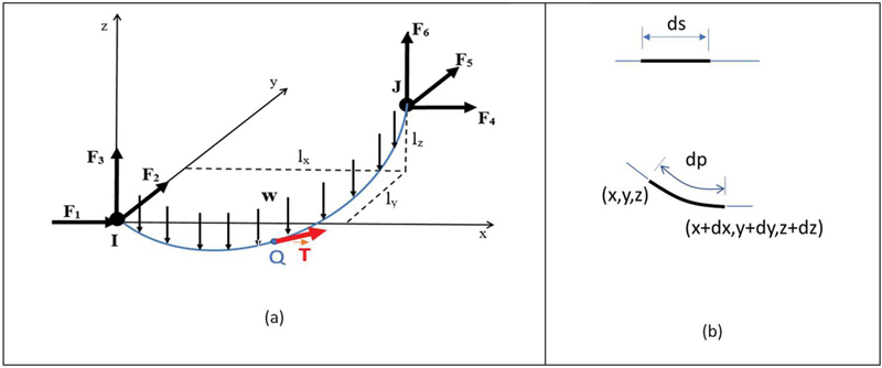
Figure 1 Three-dimensional elastic catenary cable element.

The Figure 1 shows a cable of initial length L${}_0$ suspended between two fixed points I and J which have respectively the Cartesian coordinates (0, 0, 0) and (l${}_{\mathrm{x}}$, l${}_{\mathrm{y}}$, l${}_{\mathrm{z}}$).

In the Lagrangian approach, ds and dp respectively denote the length of an infinitesimal segment of the cable in the initial and the deformed configuration (see Figure 1-b). $\overrightarrow{T}=T\overrightarrow{n}$ is the tension of the cable and represents the only mechanical action through the cross-sectional area of the cable because it is considered as perfectly flexible.

$\overrightarrow{n}=(\frac{dx}{dp},\frac{dy}{dp},\frac{dz}{dp})$ is the unit normal vector of the cross-sectional area of the cable according to the orientation from I to J.

From the above considerations, if we apply the equilibrium conditions to the part (I,Q) of the cable, we obtain the following equations:

$T\left({\displaystyle \frac{dx}{dp}}\right)$	$=-F_1$	(20a)
$T\left({\displaystyle \frac{dy}{dp}}\right)$	$=-F_2$	(20b)
$T\left({\displaystyle \frac{dz}{dp}}\right)$	$=-F_3+ws$	(20c)

From these equations, we can deduce directly:

$$T(s)=\sqrt{F_1^2+F_2^2+{(F_3+ws)}^2}$$

(21)

Furthermore, after applying Hooke’s law, we have the following equation:

$$T(s)=EA\epsilon =EA\left(\frac{dp-ds}{ds}\right)=EA\left(\frac{dp}{ds}-1\right)$$

(22)

By integrating the Equations (20) by using $\frac{dp}{ds}$ defined in Equation (22), it is established in [15] analytical expressions of $l_x,l_y,l_z$ (defined on the Figure 1) as follows:

$$l_x=f_1(F_1,F_2,F_3);l_y=f_2(F_1,F_2,F_3);l_z=f_3(F_1,F_2,F_3)$$

(23)

Note that $l_x$, $l_y$ and $l_z$ are written in function of the applied forces to the node I: $F_1,F_2$ and $F_3$.

By applying differential calculus technics, we obtain the following linear equations:

$\mathrm{\{}dl\}$	$=[W]\{dF\}\iff \left\{\begin{array}{c}\hfill d{l}_x\hfill \\ \hfill d{l}_y\hfill \\ \hfill d{l}_z\hfill \end{array}\right\}=[F]\left\{\begin{array}{c}\hfill d{F}_1\hfill \\ \hfill d{F}_2\hfill \\ \hfill d{F}_3\hfill \end{array}\right\}=\left[\begin{array}{ccc}\hfill f_{11}\mathit{\hspace{1em}}\hfill & \hfill f_{12}\mathit{\hspace{1em}}\hfill & \hfill f_{13}\hfill \\ \hfill f_{21}\mathit{\hspace{1em}}\hfill & \hfill f_{22}\mathit{\hspace{1em}}\hfill & \hfill f_{23}\hfill \\ \hfill f_{31}\mathit{\hspace{1em}}\hfill & \hfill f_{32}\mathit{\hspace{1em}}\hfill & \hfill f_{33}\hfill \end{array}\right]\left\{\begin{array}{c}\hfill d{F}_1\hfill \\ \hfill d{F}_2\hfill \\ \hfill d{F}_3\hfill \end{array}\right\},$
$f_{ij}$	$={\displaystyle \frac{\partial f_i}{\partial F_j}}$	(24)

$[W]$ represents the flexibility matrix, analytical expressions of his components $f_{ij}$ can be found in [15].

We can define now the stiffness matrix $[K]={[W]}^{-1}$ as the inverse of the flexibility matrix and then we have:

$\mathrm{\{}dF\}$	$=[K]\{dl\}\iff \left\{\begin{array}{c}\hfill d{F}_1\hfill \\ \hfill d{F}_2\hfill \\ \hfill d{F}_3\hfill \end{array}\right\}=[K]\left\{\begin{array}{c}\hfill d{u}_{Jx}-d{u}_{Ix}\hfill \\ \hfill d{u}_{Jy}-d{u}_{Iy}\hfill \\ \hfill d{u}_{Jz}-d{u}_{Iz}\hfill \end{array}\right\}\iff \left\{\begin{array}{c}\hfill d{F}_1\hfill \\ \hfill d{F}_2\hfill \\ \hfill d{F}_3\hfill \end{array}\right\}$
	$=-[K]\left\{\begin{array}{c}\hfill d{u}_{Ix}\hfill \\ \hfill d{u}_{Iy}\hfill \\ \hfill d{u}_{Iz}\hfill \end{array}\right\}+[K]\left\{\begin{array}{c}\hfill d{u}_{Jx}\hfill \\ \hfill d{u}_{Jy}\hfill \\ \hfill d{u}_{Jz}\hfill \end{array}\right\}$

Moreover from the equilibrium condition of the part (I,J) of the cable, we deduce than:

$$\{\begin{array}{c}\hfill F_4=-F_1\Rightarrow d{F}_4=-d{F}_1\hfill \\ \hfill F_5=-F_2\Rightarrow d{F}_5=-d{F}_2\hfill \\ \hfill F_6=-F_3+w{L}_0\Rightarrow d{F}_6=-d{F}_3\hfill \end{array}$$

(25)

Then we can build the tangent stiffness matrix of the cable element.

$$\{d{F}_{\mathit{int}}\}=[K_t]\{dU\}$$

(26)

With $[K_t]=\left[\begin{array}{cc}\hfill -[K]\hfill & \hfill [K]\hfill \\ \hfill [K]\hfill & \hfill -[K]\hfill \end{array}\right]$, ${\{d{F}_{\mathit{int}}\}}^T=⟨d{F}_1;d{F}_2;d{F}_3;d{F}_4;d{F}_5;d{F}_6⟩$, ${\{dU\}}^T=⟨d{u}_{Ix};d{u}_{Iy};d{u}_{Iz};d{u}_{Jx};d{u}_{Jy};d{u}_{Jz}⟩$.

The tangent stiffness matrix of the cable element is a function of the internal force vector $\{F_{\mathit{int}}\}$ which depends on the relative positions $l_x,l_y,l_z$, of the extremities I and J, on the self-weight and, of course, on the unconstrained length $L_0$. Based on the well-known catenary expressions, the initial values of the internal forces can be calculated [9] as follows:

$F_1$	$=-{\displaystyle \frac{w{l}_x}{2{\lambda }_0}}$	(27)
$F_2$	$=-{\displaystyle \frac{w{l}_y}{2{\lambda }_0}}$	(28)
$F_3$	$=-{\displaystyle \frac{w}{2}}\left(-l_z{\displaystyle \frac{\cosh {\lambda }_0}{\sinh {\lambda }_0}}+L_0\right)$	(29)

In which

$${\lambda }_0=\{\begin{array}{cc}{10}^6\mathit{\hspace{1em}}\hfill & if(l_x^2+l_y^2)=0\hfill \\ 0.2\mathit{\hspace{1em}}\hfill & if{L}_0^2\le l_x^2+l_y^2+l_z^2\hfill \\ \sqrt{3\left(\frac{L_0^2-l_z^2}{l_x^2+l_y^2}-1\right)}\mathit{\hspace{1em}}\hfill & if{L}_0^2>l_x^2+l_y^2+l_z^2\hfill \end{array}$$

(30)

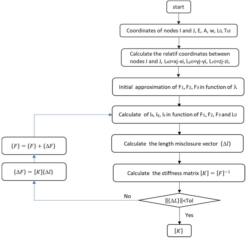
Figure 2 Flowchart of calculation the stiffness matrix of a cable element.

But $l_x,l_y,l_z$ have to satisfy also the Equations (23), which means that the final values of the internal forces can be evaluated only by an iterative procedure based on the Newton Raphson method as explicitly defined in the paper [10]. The correction of the end forces vector $\{\mathrm{\Delta }F\}$ is calculated from the misclosure lengths vector $\{\mathrm{\Delta }l\}$ by the following relation $\{\mathrm{\Delta }F\}=[K]\{\mathrm{\Delta }l\}$. The flow-chart in Figure 2 represents this iterative process.

5 Geometric Constraints

A CDPR is a specific type of robot where several cables are connecting a moving platform to fixed points A${}_{\mathrm{i}}$, A${}_{\mathrm{j}},\mathrm{\dots }$ A${}_{\mathrm{m}}$. The attachment points of the cables on the platform are denoted B${}_{\mathrm{i}}$, B${}_{\mathrm{j}},\mathrm{\dots }$ B${}_{\mathrm{m}}$.

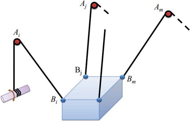
Figure 3 A general m-cable CDPR.

It is necessary, to conserve a constant distance between two end-points among B${}_{\mathrm{i}}$, B${}_{\mathrm{j}},\mathrm{\dots }$ B${}_{\mathrm{m}}$, to take into account geometric constraints in the CDPR’s modeling, as follows:

$$\mathrm{\{}R(\{U\})\}=\{F_{\mathit{ext}}\}-\{F_{\mathit{int}}\}+\{F_{\mathrm{\Phi }}\}$$	(31)
$$\mathrm{\{}\mathrm{\Phi }\}=\{0\}$$	(32)

where $\{F_{\mathrm{\Phi }}\}$ is the generalized nodal constraint forces associated to the geometric constraints represented by the algebraic Equations (32). The constraints vector $\{\mathrm{\Phi }\}$ is defined as follows:

$$\mathrm{\{}\mathrm{\Phi }\}{}^T=\{\begin{array}{ccc}\hfill (d_{ij}^2-l_{ij}^2)\mathit{\hspace{1em}}\hfill & \hfill \mathrm{\dots }\mathit{\hspace{1em}}\hfill & \hfill (d_{jm}^2-l_{jm}^2)\hfill \end{array}\}{}^T$$	(33)
$$d_{ij}^2={\{\overrightarrow{B_i{B}_j}\}}^T\cdot \{\overrightarrow{B_i{B}_j}\}$$	(34)

Where $l_{ij},\mathrm{\dots },l_{jm}$ are all the necessary lengths that must be kept constant because of the rigid motion of the platform.

Based on the formulation of the virtual work $\delta W$, we have the following relation:

$\delta W={\{\delta U\}}^T\cdot \{F_{\mathrm{\Phi }}\}={\{\delta \mathrm{\Phi }\}}^T\cdot \{\lambda \}\Rightarrow \{F_{\mathrm{\Phi }}\}={[C]}^T\{\lambda \}$

(35)

With $[C]=[\frac{\partial \mathrm{\Phi }}{\partial U}]$ is the Jacobean matrix of the geometric constraints and $\{\lambda \}$ is the Lagrangian multipliers vector in which each component represents the closure force associated to one geometric constraint.

From these previous considerations, the equations of the CDPR’s modelling becomes:

$$\mathrm{\{}\tilde{R}(\{U\})\}=\{F_{\mathit{ext}}\}-\{F_{\mathit{int}}\}+[C]{}^T\{\lambda \}$$	(36)
$$\mathrm{\{}\mathrm{\Phi }\}=\{0\}$$	(37)

To eliminate the Lagrangian multipliers, one way is to consider each closure force as proportional to the violation of the corresponding geometric constraint, as follows:

$$\{\lambda \}=-k\{\mathrm{\Phi }\}$$

(38)

Physically, it is like adding virtual springs between the cables and the moving platform at the attachment points. Fundamentally these forces are not explicit because they depend on the unknown nodal displacements. So they have to be considered as internal forces added to the others due to the cable stiffness.

$$\mathrm{\{}{\tilde{F}}_{\mathit{int}}\}=\{F_{\mathit{int}}\}+[C]{}^{T}k\{\mathrm{\Phi }\};\{\tilde{R}(\{U\})\}=\{F_{\mathit{ext}}\}-\{{\widehat{F}}_{\mathit{int}}\}$$	(39)
$$=[K_t(\{U\})]+k{[C]}^T[C]$$	(40)

This approach is the well-known penalty method in which the components of $\{\mathrm{\Phi }\}$ are called the penalty functions and $k$ the penalty factor. From now on, It is easy to apply straightforward the generalized displacement control method (GDCM).

First we solve at each iteration the following algebraic system:

$$\{\begin{array}{c}\hfill \{\mathrm{\Delta }F\}={[{\tilde{K}}_t(\{U\})]}_i^{j-1}{\{d\widehat{U}\}}_i^j\hfill \\ \hfill {\{\tilde{R}(\{U\})\}}_i^{j-1}={[{\tilde{K}}_t(\{U\})]}_i^{j-1}{\{d\overline{U}\}}_i^j\hfill \end{array}$$

(41)

Then, after having defined the right ${\lambda }_i^j$, we calculate:

$${\{dU\}}_i^j={\lambda }_i^j{\{d\widehat{U}\}}_i^j+{\{d\overline{U}\}}_i^j$$

(42)

And finally we update the quantities:

$$\{\begin{array}{c}\hfill {\{{\tilde{F}}_{\mathit{int}}\}}_i^j={\{{\tilde{F}}_{\mathit{int}}\}}_i^{j-1}+{[{\tilde{K}}_t(\{U\})]}_i^{j-1}\cdot {\{dU\}}_i^j\hfill \\ \hfill {\{U\}}_i^j={\{U\}}_i^{j-1}+{\{dU\}}_i^j\hfill \end{array}$$

(43)

The larger the stiffness parameter $k$, the lower the numerical errors of the geometric constraints (32):

$\mathrm{\{}d\mathrm{\Phi }\}$	$=[C]{\{dU\}}_i^j$
	$=[C]({([K_t(\{U\})]+k{[C]}^T[C])}^{-1}({\lambda }_i^j\{\mathrm{\Delta }F\}+{\{\tilde{R}(\{U\})\}}_i^{j-1}))$	(44)
$\underset{k\to \mathrm{\infty }}{lim}(\{d\})$	$=[C]\left({\displaystyle \frac{1}{k}}{({[C]}^T[C])}^{-1}({\lambda }_i^j\{\mathrm{\Delta }F\}+{\{\tilde{R}(\{U\})\}}_i^{j-1})\right)=\{0\}$	(45)

Because the augmented tangent stiffness $[{\tilde{K}}_t(\{U\})]$ has to be updated at each iteration, we propose another approach that we call stiffness method. We consider now the closure forces as external forces which means that must be calculated explicitly, so we propose the following increment form:

$${\{{\tilde{F}}_{\mathit{ext}}\}}_i={\{{\tilde{F}}_{\mathit{ext}}\}}_{i-1}+\mathrm{\Delta }\{F\}$$

(46)

with $\{{\tilde{F}}_{\mathit{ext}}\}=\{F_{\mathit{ext}}\}-{[C]}^{T}k\{\mathrm{\Phi }\}$ and consequently $\{\tilde{R}(\{U\})\}=$ $\{{\tilde{F}}_{\mathit{ext}}\}-\{F_{\mathit{int}}\}$

$k$ is called now the stiffness parameter.

From now on, it is easy to apply GDCM as follows:

First we solve at each iteration the following algebraic system:

$$\{\begin{array}{c}\hfill \{\mathrm{\Delta }F\}=K_t(\{U\})]{}^{j-1}{}_i\{d\widehat{U}\}{}^j{}_i\hfill \\ \hfill {\{\tilde{R}(\{U\})\}}_i^{j-1}={[K_t(\{U\})]}_i^{j-1}{\{d\overline{U}\}}_i^j\hfill \end{array}$$

(47)

Then, after having defined the right ${\lambda }_i^j$, we calculate:

$${\{dU\}}_i^j={\lambda }_i^j{\{d\widehat{U}\}}_i^j+{\{d\overline{U}\}}_i^j$$

(48)

And finally we update the quantities:

$$\{\begin{array}{c}\hfill {\{F_{\mathit{int}}\}}_i^j={\{F_{\mathit{int}}\}}_i^{j-1}+{[K_t(\{U\})]}_i^{j-1}\cdot {\{dU\}}_i^j\hfill \\ \hfill {\{U\}}_i^j={\{U\}}_i^{j-1}+{\{dU\}}_i^j\hfill \end{array}$$

(49)

As we can see the closure forces are considered in this approach like feedback external forces to control the violation of the geometric constraints which can induce numerical instabilities if these forces become too strong relative to the internal forces of the cables which occur when $k$ is too large. We have an oscillator defined by the following equation directly deduced from (44):

$\mathrm{\{}d\mathrm{\Phi }\}+[C]([K_t(\{U\})]){}^{-1}[C]{}^{T}k\{\mathrm{\Phi }\}$
$\mathrm{\hspace{1em}\hspace{1em}}=[C]({([K_t(\{U\})])}^{-1}({\lambda }_i^j\{\mathrm{\Delta }F\}+{\{F_{\mathit{ext}}\}}_{i-1}+{\{F_{\mathit{int}}\}}_i^{j-1}))$	(50)

As we can see this oscillator is strongly dependent on the inverse of the stiffness matrix and could be unstable around limit points and between snap-backs points. This method should be used only between limit points, when the load/deflection function is monotonic.

Another problem is encountered at the first increment force. Indeed, as there is not yet violation of the constraint, so there are no feedback forces. It is necessary to reduce $\{\mathrm{\Delta }F\}$ at the first increment in order to limit the violation geometric constraints at the next increment. Another possibility, safer, it is to use the penalty method at the first increment.

6 Numerical Examples

The geometric nonlinear analysis program, created for cable-supported structures, employing the 3D elastic catenary cable element, will be tested on the two first examples in order to examine its performance and also the robustness of the GDCM solver. The findings will be compared to those published in the literature.

Example 1: sagging cable

A cable is suspended between two supports 1 and 3, with a 304.8 m distance at the same level, sagging 30.48 meters. This example has been previously investigated by several researchers [9–13, 18, 19] and is taken as a validation reference for modeling nonlinear cables through different methods. The initial configuration and data for this structure is shown in Figures 4 and 1. The primary goal is to figure out the displacement at the node 2 due to the cable’s self-weight and the applied load. The tangent stiffness matrix in this case is built by connection of the two tangent stiffness matrices, one is associated to the part (1,2) of the cable and the other to the part (2,3) of the cable.

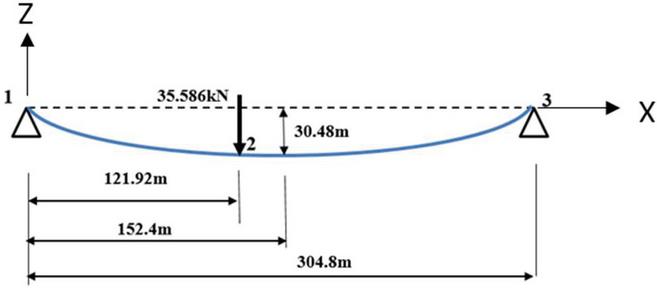
Figure 4 Example 1: two cables in 2D.

Table 1 Initial properties of each cable under concentrated load

Cross-sectional area	5.484 cm${}^2$
Elastic modulus	13100 kN/cm${}^2$
Cable self-weight	46.12 N/m
Sag under self-weight at load point 2	29.276 m
Unstressed cable length [1, 2]	125.88 m
Unstressed cable length [2, 3]	186.85 m

The load is applied incrementally until convergence, with the increment load vector $\mathrm{\Delta }$F equal to total applied forces devised by the load increment parameter p ($\mathrm{\Delta }F=\frac{F_{ext\mathit{\text{tôt}}}}{p}$). As we can see in Figure 5, p has an great influence on the solution. The greater p is, the better the solution is, with means the importance of having in the solver an increment procedure to sample the total applied forces.

The computed displacements for the node 2 under the concentrated load are compared to the existing values in Table 2. The latter shows that the current findings correspond well with those found in the literature.

Table 2 Displacement of node 2

	Displacement of Node 2
	Horizontal (m)	Vertical (m)
Reference [5]	$-$0.860	$-$5.627
Reference [4]	$-$0.859	$-$5.626
Reference [12]	$-$0.859	$-$5.626
Current results without the cable’s weight (p $=$ 10${}^4$)	$-$0.861	$-$5.641
Current results taking into account the cable’s weight	$-$0.886	$-$5.860
(p $=$ 10${}^4$)

Figure 5 presents the applied load F${}_{\mathrm{ext}}$ in function of the displacement of node 2 with p $=$ 10${}^4$ taking into account the cable’s weight.

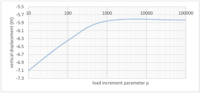
Figure 5 Vertical displacement of node 2 in function of the load increment parameter.

Example 2: cable net

Figure 6 shows a twelve-node cable net using a non-dimensional unit. At first, the cable network is in the horizontal plane (x, y). The cable net’s attributes are expressed in consistent units as the following: the cross-sectional area A is 1 unit, the elastic modulus E is 29.10${}^5$ units, the initial length of each cable is L${}_0$ $=$ 40 units and the self-weight w is 1 unit. At node 8, a load of 1000 units is applied in the opposite direction of z.

Figure 6 12 cables in 3D.

Table 3 shows the displacements of internal nodes and the comparison of the results found to references [13] and [17]. The acquired findings are extremely similar to those supplied by the references.

Table 3 Displacement of cable net’s internal nodes

	Current Results (p $=$ 10${}^4$)			[17]			[13]
Node	$u{}_x$	$u{}_y$	$u{}_z$	$u{}_x$	$u{}_y$	$u{}_z$	$u{}_x$	$u{}_y$	$u{}_z$
4	$-$0,01424	$-$0,02967	$-$1,63223	$-$0,01420	$-$0,02959	$-$1,63049	$-$0,014	$-$0,03	$-$1,631
5	0,00392	0,00392	$-$1,35867	0,00393	0,00393	$-$1,35768	0,004	0,004	$-$1,359
8	$-$0,06283	$-$0,06283	$-$3,1761	$-$0,06269	$-$0,06269	$-$3,17212	$-$0,063	$-$0,063	$-$3,175
9	$-$0,02966	$-$0,0142	$-$1,63223	$-$0,02959	$-$0,0142	$-$1,63049	$-$0,03	$-$0,014	$-$1,632

Table 4 Example2: Error percentage compared to references for node 4

	$u{}_x$	$u{}_y$	$u{}_z$
Error percentage compared to	0,2817 %	0,27%	0,107%
Damir Seldar et al. [17] for node 4
Error percentage compared to	1,71%	1,1%	0,0754 %
Y.B. Yang et al. [13] for node 4

To verify each method’s feasibility, multiple tests were concluded. The main focus for the next two examples is to verify the results found in example 2 by considering geometric constraints. The value of p chosen is 10${}^4$ for the following examples.

Example 3: Cable net with linear geometric constraints

In the example 2, all the degrees of freedom of the nodes 1, 2, 3, 6, 7, 10, 11, 12 are set to zero and so are eliminated in the modelling of the cable net. In this example the node 1 is now considered to be attached to the fixed support. Its three degrees of freedom in translation are not eliminated but constrained by three forces in translation. The three algebraic constraints that we have to take into account in this modelling, are u${}_{\mathrm{1}\mathit{}x}$ $=$ 0, u${}_{\mathrm{1}\mathit{}y}$ $=$ 0 and u${}_{\mathrm{1}\mathit{}z}$ $=$ 0. We can note that they are linear relative to the DOF and not nonlinear as previously defined in the case of maintaining distance between two nodes. Just like in Example 2, a load was applied to the node 8 with the value of 1000 units in the opposite direction of the z axis.

The results found in this example were compared and verified by the results found with the original GDCM. Table 7 represents the nodes’ displacement found using the stiffness method with k $=$ 10${}^6$ and the nodes’ displacement found using the penalty method with k $=$ 10${}^{10}$ compared to the results found in example 2. It is noted that each time k is increased, the precision improves. However, both methods have limits. For the stiffness method, when k is above 10${}^6$, the displacement’ values diverge. This is noted throughout several results found for this method. However, for this type of case, the penalty method doesn’t have limits concerning increasing the value of k.

Table 5 Result found after fixing node 1

	Stiffness Method			Penalty Method			Results Found in Example 2
Nodes	u${}_x$	u${}_y$	u${}_z$	u${}_x$	u${}_y$	u${}_z$	u${}_x$	u${}_y$	u${}_z$
1	$-$2,18E-06	$-$0,003	$-$0,0002	$-$1,62E-10	$-$3,99E-07	$-$2,06E-08	0	0	0
4	$-$0,0142	$-$0,0318	$-$1,634	$-$0,0142	$-$0,0297	$-$1,6322	$-$0,0142	$-$0,0296	$-$1,632
5	0,00387	0,0038	$-$1,358	0,0039	0,0039	$-$1,3587	0,0039	0,0039	$-$1,358
8	$-$0,0631	$-$0,0641	$-$3,182	$-$0,0628	$-$0,0628	$-$3,1761	$-$0,0628	$-$0,0628	$-$3,176
9	$-$0,0298	$-$0,0142	$-$1,633	$-$0,0297	$-$0,0142	$-$1,6322	$-$0,0296	$-$0,0142	$-$1,632

It is worth noting that the displacement found in both scenarios is highly similar to the GDCM, however, Table 8 proves that the penalty method shows better results.

Table 6 Example 3: Error percentage for node 4 compared to results found in example 2

	u${}_x$	u${}_y$	u${}_z$
Error percentage for node 4 with the stiffness method	0,0 %	$-$7,43%	$-$0,12%
Error percentage for node 4 with the penalty method	0,0 %	$-$0,34%	$-$0,01%

Figure 7 A cable net with 6 geometric constraints.

Example 4: Cable net with nonlinear geometric constraints

we consider now, six non linear geometric constraints inside the cable net previously defined in the example 2. These six constraints keep the distances respectively between (4, 5), (5,9), (9,8), (8,4), (4,9) and (8,5). In that way, it is like we have a square rigid platform suspended by eight cables (bleu links) which are respectively (3,4), (7,8), (1,4),(2,5), (5,6), (9,10), (9,12) and (8,11).

At node 8, the same load is applied in the opposite direction of z than in the first example.

As shown in Table 7, the results found between the two methods are similar and coherent with the result from the original example. Similar to other tests, the stiffness method has a limit value for k (no more than 10${}^6$). In addition, the value of k for the penalty method is limited to no more than 10${}^{12}$.

Evidently, the penalty method proves to be the more accurate method. These results indicate the suggested programs’ good computational efficiency in different cases.

Table 7 Nodal displacements

	Stiffness Method			Penalty Method
Nodes	u${}_x$	u${}_y$	u${}_z$	u${}_x$	u${}_y$	u${}_z$
4	$-$0,02683	$-$0,02762	$-$1,32615	$-$0.0218	$-$0.0218	$-$1.525
5	$-$0,02980	$-$0,02980	$-$0,77438	$-$0.0369	$-$0.0369	$-$0,427
8	$-$0,00814	$-$0,00814	$-$2,67144	$-$0,0067	$-$0,0067	$-$2,628
9	$-$0,02762	$-$0,02683	$-$1,32615	$-$0,0218	$-$0,0218	$-$1,526

Table 8 Computed distances between nodes

		Final Distances
	Initial Distances	Stiffness Method	Penalty Method
4 and 5	40	40,0008	40
4 and 8	40	40,0031	40
4 and 9	56,5685	56,5674	56,5686
5 and 8	56,5685	56,5697	56,5686
5 and 9	40	40,0008	40
8 and 9	40	40,0031	40

7 Conclusion

Due to the flexible nature of cable-supported structures, the geometric nonlinear impact must be considered while analyzing them. The Generalized Displacement Control method (GDCM), was used to perform incremental-iterative analysis where the loads are not kept constant in the iterative steps and general numerical stability is maintained when passing limit points and snap-back points. Three different tests on cable structures were presented, where the results were compared to previous results found by other researches. Through this comparison, it was found that the GDCM using a 3D elastic catenary model is verified. In addition, two modifications of this method were applied to take into account geometric constraints equations coupling the large displacements of the cable ends. The first method presented to eliminate the geometric constraints consisted by using the penalty function method while in the second method adding external explicit elastic forces were considered. These two methods were tested and verified by different numerical examples. From a numerical point of view, the first method is safer because it is not dependent on the poor numerical conditioning of the stiffness matrix which occurs around limit points and between snap-backs points. For future work, the aim is to implement the augmented Lagrangian technique to control the numerical error of the nonlinear geometric constraints. In addition, we have also, the objective to model a CDPR using the methods presented earlier in this paper.

Acknowledgement

The authors would like to thank Zhi-Qiang FENG Professor at the University of Evry for his help during this study.

Funding

This work is supported by a public grant overseen by the French National research Agency (ANR) as part of the “Investissements d’Avenir” program, through the “ADI 2019” project funded by the IDEX Paris-Saclay, ANR-11-IDEX-0003-02” and the University of Tunis El Manar.

References

[1] F. BenAbdallah, N. Azouz, L. Beji and A. Abichou, “Modeling of a heavy lift airship carrying a payload by a cable driven parallel manipulator,” International Journal of Advanced Robotic Systems, 2019.

[2] N. Azouz, M. Khamlia, F. B. Abdallah and F. Guesmi, “Modelling and design of an airship crane,” in ASME-IMECE Conference, Pittsburgh, USA, 2018.

[3] H. Yuan, E. Courteille and D. Deblaise, “Static and Dynamic Stiffness Analyses of Cable-Driven Parallel Robots with non-negligible cable mass and elasticity,” Mechanism and Machine Theory, pp. 64–81, 2015.

[4] S. Bouchard and C. M. Gosselin, “Kinematic sensitivity of a very large cable-driven parallel mechanism,” in ASME International Design Engineering Technical Conferences, 2006.

[5] D. Q. Nguyen, M. Gouttefarde, O. Company and F. Pierrot, “On the Simplifications of Cable Model in Static Analysis of Large Dimensions Cable-Driven Parallel Robots,” in IEEE/RSJ International Conference on Intelligent Robots and Systems (IROS), Tokyo, Japan, 2013.

[6] R. Nicolas, G. Marc, K. Sébastien, B. Cédric and P. François, “Effects of non-negligible cable mass on the static behavior of large workspace cable-driven parallel mechanisms,” in IEEE International Conference on Robotics and Automation, Kobe, Japan, 2009.

[7] M. Gouttefarde, J.-F. Collard, N. Riehl and C. Baradat, “Simplified Static Analysis of Large-Dimension Parallel Cable Driven Robots,” in IEEE International Conference on Robotics and Automation, Minnesota, USA, 14–18 May, 2012.

[8] M. Irvine, Cable Structures, New York: dover publications, Inc, 1981.

[9] H. Jayaraman and W. Knudson, “A Curved Element for the Analysis of Cable Structures,” Computers & Structures, vol. 14, no. 3–4, pp. 325–333, 1981.

[10] H.-T. Thai and Seung-EockKim, “Nonlinear Static and Dynamic Analysis of Cable Structures,” Finite Element in Analysis and Design, vol. 47, pp. 237–246, 2011.

[11] E. Coarita and L. Flores, “Nonlinear Analysis of Structures Cable-Truss,” International Journal of Engineering and Technology, pp. 160–169, 2015.

[12] Z. Wu and J. Wei, “Nonlinear Analysis of Spatial Cable of Long-Span Cable-Stayed Bridge considering Rigid Connection,” KSCE Journal of Civil Engineering, pp. 2148–2157, 2019.

[13] Y. B. YANG and J.-Y. TSAY, “Geometric Nonlinear Analysis of Cable Structures with a Two-node Cable Element by Generalized Displacement Control Method,” International Journal of Structural Stability and Dynamics, vol. 7, no. 4, pp. 571–588, 2007.

[14] C. M. Hoffmann and R. Joan-Arinyo, Handbook of Computer Aided Geometric Design, 2002.

[15] M. A. Torkamani and M. Sonmez, “Solution Techniques for Nonlinear Equilibrium Equations,” in 18th Analysis and Computation Specialty Conference, 2008.

[16] Y.-B. Y. a. M.-S. Shieh, “Solution Method for Nonlinear Problems with Multiple Critical Points,” AIAA JOURNAL, vol. 28, no. 12, pp. 2110–2116, 1990.

[17] S. Damir, L. Zeljan and B. Andjela, “Nonlinear static isogeometric analysis of cable structures,” Archive of Applied Mechanics, vol. 89, p. pages 713–729, 2019.

[18] H.-T. Thai and S.-E. Kim, “Nonlinear static and dynamic analysis of cable structures,” Finite Elements in Analysis and Design, vol. 47, p. 237–246, 2011.

[19] A. A. M. Salehi, A. Shooshtari, V. Esmaeili and N. R. Alireza, “Nonlinear analysis of cable structures under general loadings”, Finite Elements in Analysis and Design, vol. 73, pp. 11–19, 2013.

[20] J.L. Batoz, G. Dhatt, “Incremental displacement algorithms for nonlinear problems”, International Journal for Numerical Methods in Engineering, vol. 14, pp. 1262–1267, 1979.

Biographies

Pierre Joli Assistant professor at the Evry_Paris-Saclay University. His activities within the LMEE Laboratory cover several areas of non linear computational solid mechanics. He has published articles dealing with frictional contact and large deformation mechanical problems, particularly in the case of hyperelastic material. He is responsible for the IC2M Master at Evry Paris-Saclay University.

Naoufel Azouz Associate professor at the Evry_Paris-Saclay University. He obtained the PhD of PhD of the university Paris 6 in cooperation with the Atomic Center of Saclay, France in 1994. In 1995 he joined the university of Evry in France, where he is now teaching in the mechanical department. His research interests are structural dynamics and aerodynamics modeling of flying objects. His researches are done in the LMEE laboratory in Evry, France.

Manel Ben Wezdou PhD student in joint supervision between the University of Evry_Paris-Saclay and the University of Tunis_El-Manar. Her field of research concerns the development of numerical algorithms for the static and dynamic modeling of heavy flexible cables.

Jamel Neji Full professor in Civil Engineering at the National School of Engineers of Tunis. He has published papers on a wide range of disciplines, in particular (design of pavement structures; dynamic study of railway structures; cracking of materials; rigidity of composite materials; transport infrastructures). He is director of the Civil Engineering department at ENIT and head of the Materials, Optimization and Energy for Sustainability Laboratory (LAMOED).

European Journal of Computational Mechanics, Vol. 31_4, 433–458.
doi: 10.13052/ejcm2642-2085.3141
© 2023 River Publishers

Abstract

1 Introduction

2 Notations

3 Algorithm for Nonlinear Equilibrium Equations

4 Elastic Catenary Cable

5 Geometric Constraints

6 Numerical Examples

Example 1: sagging cable

Example 2: cable net

Example 3: Cable net with linear geometric constraints

Example 4: Cable net with nonlinear geometric constraints

7 Conclusion

Acknowledgement

Funding

References

Biographies