Application of GA-BP in Displacement Force Inverse Analysis and Mechanical Parameter Inversion of Deep Foundation Pits
Guo Yunhong* and Zhang Shihao
Railway Engineering College, Zhengzhou Railway Vocational & Technical College, Zhengzhou 450052, China
E-mail: xscgyh@163.com
*Corresponding Author
Received 17 April 2023; Accepted 19 May 2023; Publication 22 June 2023
Abstract
Aiming at the defects of various existing displacement inverse analysis methods, using the nonlinear mapping ability of neural network and the global random search ability of genetic algorithm, this paper proposes a displacement inverse analysis method based on optimized Genetic Algorithm- Back Propagation (GA-BP) for deep foundation pit support. The method changes the method that BP algorithm relies on the guidance of gradient information to adjust the network weights, but uses the characteristics of global search of genetic algorithm to find the most suitable network connection rights and network structure, etc. to achieve the purpose of optimization. Firstly, the deformation mechanism of deep foundation pit is analyzed, its failure mode is summarized, and the calculation method of lateral rock and soil pressure is sorted out according to the code. The theory and characteristics of BP neural network and genetic algorithm are discussed, and the method of using genetic algorithm to optimize BP neural network is proposed to improve the prediction accuracy. In view of the shortcomings of GA-BP neural network prediction model in training sample pretreatment and hidden layer structure design, the optimal normalization interval was determined by correlation coefficient regression analysis, and the analytical expression of the number of neurons in hidden layer was derived by statistical principle, and the value range of the optimal number of neurons in single hidden layer was proposed. Combined with the actual engineering, the mechanical parameters inversion and displacement force inverse analysis are performed using this method, and the results show that the optimized GA-BP has higher prediction accuracy compared with BP neural network and GA-BP, and the deviation of the displacement prediction value at each depth is kept within 0.2 mm, the absolute error interval width is 0.07 mm, and the maximum relative error is 1.35% at 4.0 m depth.
Keywords: Mechanical parameters, displacement force, inverse analysis, optimization GA-BP, deep foundation pit.
1 Introduction
As China’s construction industry advances, the depth of excavation for several subway pits is increasing significantly, and the issues encountered are turning into greater and extra prominent. In the normal format of deep basis assist methods, the calculation is typically carried out in accordance to the pressure electricity and normal stability. There are many soils mechanical parameters involved, and they are at once associated to the protection and economic system of the guide shape for an aid scheme [1]. Therefore, it is vital to use the displacement values measured in the area and follow the displacement inverse evaluation approach to invert the mechanical houses of the soil in accordance to the chosen intrinsic model, and then alter the aid scheme to ensure the security of the basis pit. The present displacement inverse evaluation techniques have shortcomings; the displacement inverse evaluation approach primarily based on optimization idea has terrible steadiness of the solution, effortless to fall into nearby minima, gradual convergence when there are many inverse parameters, and hard to search for the best answer [2]; the displacement inverse analysis method based on artificial neural network is difficult to converge to the required accuracy when the solution space is a little larger, so it is difficult to obtain the inversion results consistent with the actual rock and soil. The displacement inverse analysis method based on genetic evolution requires a lot of empirical intervention in the search process to search for the optimal solution.
Currently, Shen Hsiu-Chung, on the basis of detailed analysis of the spatio-temporal effect influencing factors, tried to establish a spatio-temporal effect analysis model for deep foundation pits using an evolutionary algorithm to optimize the neural network structure and initial weights in steps [3]; Xue X et al. proposed a approach based totally on a hybrid GA-BP algorithm to predict the mechanical houses of heavy-duty wheel-rail wear, simplified the wheel-rail contact relationship the usage of Hertz contact theory, and hooked up a wheel-rail contact mannequin [4]; Yanjie Li et al. optimized the preliminary weights and thresholds of the BP neural community the use of genetic algorithm, and organized a pit deformation prediction software the usage of MATLAB, installed a neural community mannequin about the horizontal displacement of the enclosure shape of the underground diaphragm wall of the deep basis pit, and estimated the horizontal displacement of the enclosure shape corresponding to a measured slant gap of the pit prediction [5]; Daneshkhah E et al. introduced and mentioned the theoretical evaluation primarily based on NASA SP-8007 answer and the simplified equations for cylindrical buckling from ASME RD-1172, the consequences of theoretical and finite factor evaluation and experimental exams evaluating glass and carbon epoxy resin cylinders [6]; Song Chuping proposed the application of BP neural network to solve the nonlinear and uncertainty problems of foundation pit deformation, taking into account both the main independent variables of foundation pit deformation and the ductility of the model in time in the process of BP model construction [7]; Kalanad A et al. proposed an improved two-dimensional (2-D) finite element (FE) based crack diagnosis method with embedded edge cracks and a microscopic genetic algorithm (-GA) [8].
Aiming at the defects of a number current displacement inverse analysis methods, the use of the nonlinear mapping capability of neural community and the world random search potential of genetic algorithm, this paper proposes a displacement inverse evaluation technique primarily based on optimized GA-BP for deep basis pit support. The technique adjustments the approach that BP algorithm depends on the practice of gradient data to regulate the community weights, however makes use of the traits of world search of genetic algorithm to locate the most appropriate community connection rights and community structure, etc. to acquire the reason of optimization. Firstly, this paper analyzes the deformation mechanism of deep basis pit, outlines its injury mode, and organizes its lateral geotechnical strain calculation technique in accordance to the specification; discusses the precept and features of BP neural neighborhood and genetic algorithm, and proposes the use of genetic algorithm to optimize the BP neural neighborhood to decorate the prediction accuracy. To handle the shortcomings of the GA-BP neural neighborhood prediction model in teaching sample preprocessing and hidden layer structure design, the great normalization interval is determined by using correlation coefficient regression analysis, the analytic device of the extent of neurons in the hidden layer is derived by means of the use of statistical principles, and the range of the most extraordinary range of neurons in the single hidden layer that is nicely appropriate with it is proposed. Combined with the genuine engineering, the mechanical parameters inversion and displacement pressure inverse evaluation are performed the use of this method, and the outcomes exhibit that the optimized GA-BP has higher prediction accuracy in contrast with BP neural community and GA-BP, and the deviation of the displacement prediction price at every depth is stored inside 0.2 mm, the absolute error interval width is 0.07 mm, and the most relative error is 1.35% at 4.0 m depth.
2 Deformation Mechanism and Damage Mode of Deep Foundation Pit
2.1 Foundation Pit Deformation Mechanism
(a) Deformation of enclosure structure
The excavation of the basis pit will spoil the equilibrium nation of the soil, exchange the stress of the soil internal and outdoor the basis pit in the horizontal direction, and reason the redistribution of soil stress. Moreover, with the gradual excavation, stress distinction will be generated on each facets of the enclosure structure, which will lead to lateral displacement of the shape and then reason the motion of the strata round the pit [9]. During the excavation of the basis pit, energetic earth stress will be generated on the outdoor of the enclosure shape above the excavation floor of the basis pit, and the earth strain will progressively enlarge with the depth of the excavation of the basis pit and be allotted in a triangular or trapezoidal shape; whilst under the excavation floor of the basis pit, the soil on the inner of the enclosure shape will be subjected to passive earth pressure, and the stress distinction generated inner and outdoor the soil will motive the soil to pass towards the aspect of the enclosure structure, as a result inflicting the enclosure shape to produce horizontal displacements. Therefore, the deformation of the enclosure shape is by and large the horizontal displacement relative to the internal and outer aspects of the pit wall. The displacement of the enclosure shape is tremendously small due to the fact the pressure trade in the vertical course is small [10]. However, the monitoring and evaluation of the vertical displacement of the enclosure shape have to be unnoticed in the development of basis pit tasks to keep away from the hidden threat of the generated vertical displacement on the floor agreement round the pit and the standard steadiness of the enclosure structure.
The deformation of the basis pit enclosure shape is now not solely affected by using the surrounding environment, development procedure and weather, however additionally associated to the shape of aid shape and fabric properties. Clough G W [11] summarized the deformation of the enclosure shape and interior aid in exceptional excavation stages, and summarized the displacement types of the enclosure shape into three types: cantilever, parabolic and combined, as proven in Figure 1.
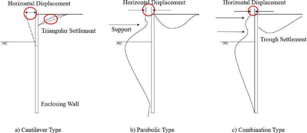
Figure 1 Displacement form of enclosure structure.
In the early stage of basis excavation, when the excavation depth is shallow or no inner help is set, the displacement of the enclosure shape is cantilevered. At this time, the most horizontal displacement will show up at the pinnacle position, and progressively decreases alongside the vertical direction, with a linear distribution, and the horizontal displacement contour line gives an inverted triangle shape. With the make bigger of excavation depth and the gradual putting of inside support, the displacement of the enclosure shape will trade and the most price will cross downward, roughly placed in the center of the basis pit. In this process, the most floor contract will show up inside a positive vary of the enclosure structure. The horizontal shift and floor contract displacement distribution curve of the enclosure shape indicates a parabolic form. When the excavation depth of the pit continues to amplify and extra anchors are set, the enclosure shape will exhibit a mixed displacement structure of cantilever kind and parabolic kind below the motion of horizontal stress [12]. However, the displacement monitoring of some basis pit tasks is carried out regularly after the construction, so the deformation in the monitoring records may additionally nonetheless existing a parabolic type.
(b) Peripheral surface settlement
During the excavation of the groundwork pit, the displacement alternate of the enclosure form will exchange the stress state of the soil spherical the pit, and the plastic waft of the soil will increase. Under the motion of lively soil strain backyard the enclosure structure, the soil on the outdoor of the pit will pass into the pit, and the soil will sink, for this reason inflicting the soil round the pit to produce one of a kind stages of agreement deformation. In addition, the building round the basis pit will additionally lead to displacement adjustments in the soil layer and produce corresponding floor contract [13]. According to the excavation depth and the unique guide structures, the deformation varieties of floor agreement round the basis pit are more often than not divided into: triangular agreement and groove-shaped settlement.
When the Morphing of the fence shape is large, the soil at the pinnacle of the pit slope will cross to the interior of the pit for filling the phase in contact with the enclosure structure, and at this time, the agreement shape in the main indicates triangular form [14]. The triangular contract has the biggest displacement at the pinnacle of the wall, and the contract will steadily reduce alongside the course away from the pit, as proven in Figure 2(a). The assist shape can be simplified to a really supported beam when the reinforcement shape is deep into the soil or embedded in the soil with excessive stiffness. Under the motion of inner support, the agreement deformation close to the basis pit will be incredibly small. At this time, the vicinity of the most agreement cost of the surrounding floor is at a positive distance from the pit wall, which is commonly placed inside 0.40.7 instances of the excavation depth, as proven in Figure 2(b).
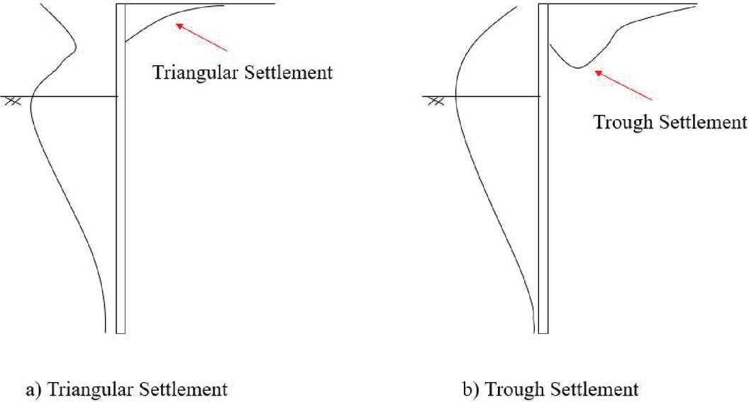
Figure 2 Peripheral surface settlement form.
(c) Base elevation at the bottom of the pit
The digging of the basis pit will produce unloading impact in the vertical course and break the authentic stress stability at the backside of the basis pit, ensuing in special ranges of uplift at the backside of the basis pit. Moreover, with the growing excavation depth, the surrounding soil will additionally always squeeze the backside of the pit underneath the motion of its personal gravity, inflicting the backside of the pit to bulge [15]. In addition, when the protecting measures of the enclosure shape are now not perfect, section of the groundwater will attain the backside of the pit thru the water end curtain. Under the motion of water, the backside of the basis pit will additionally produce uplift deformation. The bottom of the basis pit will be deformed through water, such as two kinds of elastic deformation and plastic deformation.
In the early stage of excavation, the soil unloading quantity is incredibly small, and the stress alternate at the backside of the pit is now not large. Base pit backside uplift is more often than not the elastic uplift triggered through the unloading motion of a single soil physique [16]. When the soil fantastic is good, the enclosure shape will be raised correspondingly with the uplift of the soil at the backside of the basis pit, and the elastic uplift is in general manifested as a large uplift in the center place at the backside of the basis pit and small on each side, as proven in Figure 3(a). When the excavation depth continues to increase, the excavation floor of the pit will maintain shifting downward, and below the motion of stress difference, the soil on the backyard of the pit will cross to the inner of the pit. In this process, the elevation at the backside of the pit regularly adjustments from elastic to plastic, and will be accompanied by means of the lengthwise agreement movement of the soil round the pit. At this time, the most uplift at the backside of the pit is placed on each side, and the central uplift is smaller, as proven in Figure 3(b).
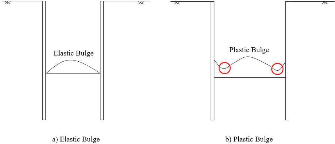
Figure 3 Schematic diagram of the rise at the bottom of the foundation pit.
2.2 Pit Damage Mode
(a) Damage mode of soil foundation slope
Soil basis slope skill the total slope is composed of soil, which can be divided into clay slope, loess slope, expansive soil slope and mounded soil slope in accordance to soil type. The harm mode of these slopes is more often than not manifested as slump, landslide and collapse.
Collapse is a layer-by-layer deformation phenomenon caused by external forces such as water in soil, crack water, vibration and excavation of artificial soil, which leads to the increase of soil weight and the decrease of soil strength and cannot maintain the stability of slope. Slope sliding often occurs when rock and soil mass collapses. By checking the collapse when there is no obvious sliding surface to distinguish the collapse and sliding.
Sliding is a phenomenon in which the geotechnical physique of a slope loses its unique secure country and slides alongside a sliding floor or sliding region as a complete underneath the motion of gravity, rainwater, groundwater, building vibration or different exterior forces, when the sliding pressure generated by means of a sliding floor or a sliding sector is larger than the corresponding sliding pressure on the sliding floor or sliding quarter [17]. The sliding floor can be divided into airplane sliding, folding sliding, round sliding and extra complicated composite sliding, as proven in Figure 4.

Figure 4 Landslide types.
(b) Damage pattern of stratified rock foundation pit
Experts and students in China have made extra achievements in the lookup on the harm sample and harm kind of laminated rock basis slope. According to the classification techniques of instability of distinctive pit slopes, the harm sorts of laminated rocky pit slopes can be divided into distinctive types.
Based on the form of the slip surface, it can be divided into the following categories:
Plane sliding: the synthetic foundation slope formed after the foundation excavation, the rock of the slope slides along a single slip layer, and a hazardous phenomenon occurs. The slip floor right here is mostly a layer with negative mechanical homes or a susceptible interlayer, and this kind of harm on the whole happens in laminated pits with tendency. As proven in Figure 5(a).
Arc sliding: Many specialists and pupils have studied and concluded that such harm normally happens in pits with fractured or free laminated rock our bodies with developed stages and joints. Arc-slip injury can appear in horizontally (near-horizontally) produced rocky footings or counter-trending rocky footings, as proven in Figure 5(b).
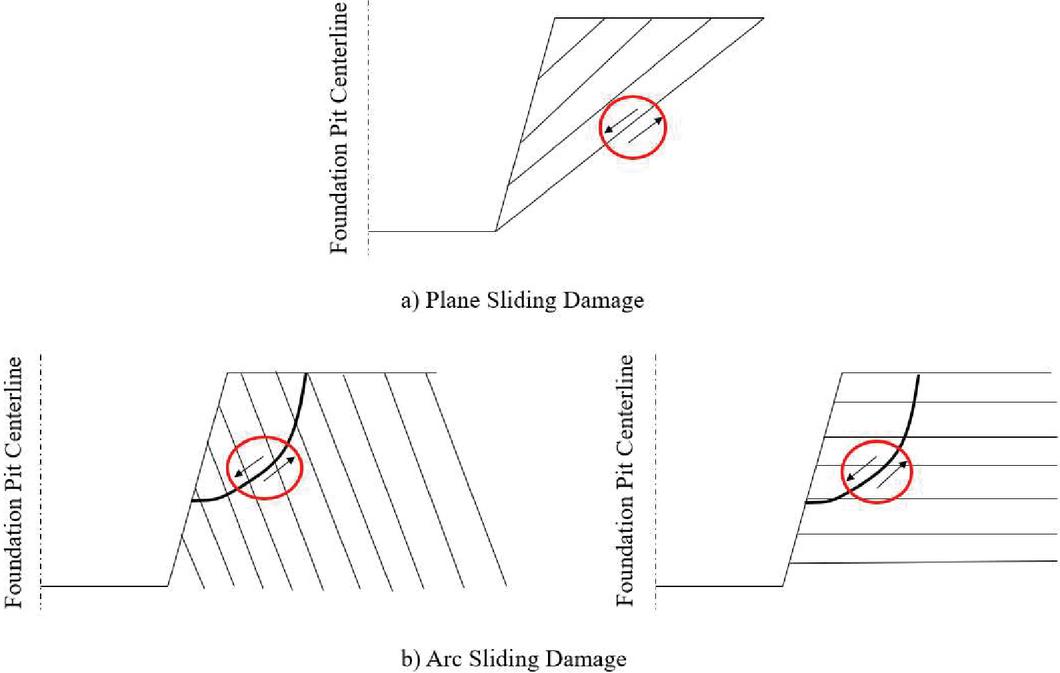
Figure 5 Damage pattern by slip surface shape.
Wedge (block) sliding: Wedge (block) sliding damage is one of the common damage modes of tangential rock foundation and down-trending rock foundation. According to the spatial geometry of the damaged rock mass, it can be divided into two types: a block and a wedge, wherein the wedge is cut from two or more structural faces and will slide along two structural faces in the same direction as the direction of intersection of the two constitutional faces. The block is cut from three or more structural faces and will slide in the direction of the cross line of the structural faces whose inclination angle is less than the slope angle of the pit wall.
Pit wall settlement damage: At the level of rock layer level or nearly level and there is under lying soft interlayer, when the pit is excavated, the soft interlayer material between rock layers produces plastic flow into the pit, which leads to the overhang of the upper laminated rock body, and the laminated rock body bends and fractures under the action of external force. After the fracture of the rock body occurs, uneven settlement of the surface around the foundation pit or tilt damage of the surrounding buildings often occurs.
2.3 Calculation of Lateral Geotechnical Pressure
Calculation of static earth pressure:
| (1) |
Where: is the static earth pressure at the calculation point (KN/m); is the weight of the jth layer of soil above the calculation point (KN/m); is the thickness of the jth layer of soil above the calculation point (h); q is the additional mean load at the top of the slope (KN/m); is the coefficient of static earth pressure at the calculation point.
Starting from the assumption of plane slip cracking surface, the active earth pressure combined force is formulated as follows:
| (2) | ||
| (3) | ||
| (4) | ||
| (5) |
Where: is the active earth pressure combined force corresponding to the standard combination of loads (KN/m); is the active earth pressure coefficient; H is the height of retaining wall (m); c is the cohesive force of soil (kPa).
For the slope sliding along the outward sloping structural surface, it is necessary to calculate its active rock pressure coefficient by two calculation methods and take the maximum value. The outward inclined structural surface generally refers to the structural surface whose inclination is less than 30 from the inclination of the broken surface.
The calculation is as follows:
| (6) | ||
| (7) | ||
| (8) |
Where: is the inclination angle () of the slope inclined structure surface; the cohesive force (kPa) of the slope inclined structure surface; is the internal friction angle () of the slope inclined structure surface.
For rocky slopes without outwardly inclined structural surface, the equivalent internal friction angle of the rock body is calculated by substituting the formula of lateral earth pressure in Equation (2)–(5).
3 GA-BP Neural Network Model
3.1 BP Neural Network
Input layer, hidden layer and output layer constitute the topology structure of BP neural network. The work consists of two steps: forward propagation stage: input information is first inputted into the input layer, and is gradually processed in each hidden layer to obtain the actual output value of each unit; Back propagation stage: If the desired output value meeting the requirements cannot be calculated, the difference between the actual output and the desired output will be converted step by step [18]. The errors will be reversed and propagated from the output layer to the input layer in turn, and the weight and threshold values will be corrected while propagating to reduce the errors between the output and the expected output. The cycle will continue until there are two kinds of network results to complete the training, one is that the expected output results meet the expected standard, the other is to reach the preset training times. Finally, the prediction results can be calculated directly by inputting the data into the trained network.
As shown in Figure 6, the most basic BP model is composed of three layers, i.e., the input level, the implicit level, and the output level. The basic algorithm of the web is the error back propagation algorithm, which is essentially an error gradient descent optimization method.
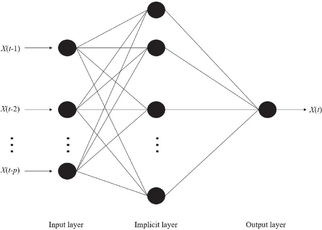
Figure 6 Schematic diagram of BP network.
In the selection of the activation function, it is generally necessary to have a continuously derivable nonlinearity, so the standard Sigmoid-type function is often chosen:
| (9) |
where is the state of the network cell:
| (10) |
Then the output unit is:
| (11) |
where is the threshold value of the cell.
Under this excitation function, there are:
| (12) |
Therefore, the error is found for the output unit:
| (13) |
For the hidden level cells find the error:
| (14) |
The weights are adjusted as follows
| (15) |
where represents the learning rate, and an increase in directly leads to a larger and more dramatic change in the weights. In fact, an additional “potential term” is often attached to while taking into account the need to not produce drastic changes and to increase the learning rate.
The error back-propagation learning process completes the input-to-output mapping through a process that minimizes the energy function. In this paper, the energy function is defined as the mean square error of the output layer unit, and with learning samples, then
| (16) |
where: , are the actual output and the desired output of sample , respectively.
The acquisition process of BP network consists of a forward calculation process and an error back propagation procedure. The procedure of learning is as follows:
(1) Network priming: input study rate , momentum factor a; given largest learning mistake (convergence accuracy); given each edge connection weight ; neuron threshold for small random values;
(2) Provide learning samples for the network: i.e., input vector , and output vector ;
(3) Compute the actual output of the network:
Implicit layer:
| (17) |
Output layer:
| (18) |
where: ; ; is the Sigmoid function.
Error in each layer:
| (19) | ||
| (20) |
Adjusting the weights of the edges:
(4) Calculate the network error E
(5) Judgment: if , learning is finished; otherwise, go to (3).
3.2 Genetic Algorithm
Genetic algorithm (GA) uses “chromosomes” to simulate and express the problem to be solved. Ga starts from strings of “chromosomes” carrying a fixed population number and places them in the “set” of the problem to be solved [19]. According to the natural selection law of survival of the fittest, those “chromosomes” that can meet the environmental requirements are selected from the population, and continue to reproduce. Then, by using the three genetic operations of selection, variation and crossover, the “chromosome” group species with better new adaptation to the environment than the previous generation is evolved. Recall that the whole process of computing is like the evolution of selection in biological species, where those with excellent quality in line with the best solution tendency of the question to be solved are continuously passed on, while those not adapted to the algorithm function are eliminated from the game. Evolutionary selection, the previous generation of individuals in the chromosome with distinctive features that help improve the degree of adaptation of the information is inherited without reservation to the offspring, the biggest difference between the two generations of individuals is that the corresponding new generation of individuals will always be in the overall adaptation of the parent beyond, so that the entire population can promote the continuous optimization of the development of the good direction. This is reflected in the genetic algorithm, which is expressed as the process of continuous tendency to approach the optimal solution.
Based on the basic idea of genetic algorithm, its basic steps are described as follows:
1. Encoding. Choose a suitable encoding method or encoding strategy to encode the phenotypes of individuals into the corresponding chromosomes (genotypes) in the population, and get the initial population.
2. Set the basic parameters of the genetic algorithm. These include population size (i.e., population size), maximum number of evolutions, iteration termination criterion, selection method, crossover method and crossover probability, variation method and variation probability, etc.
3. construct a suitable fitness function according to the actual problem. Generally, refer to the objective function to construct.
4. Calculate the individual fitness value with reference to the fitness function constructed in step 4.
5. Genetic evolutionary operations: selection, crossover, and variation. After completing these three operations, the new generation population is obtained.
6. Perform the judgment operation on the new population in the algorithm. If not, return to repeat step 4 and step 5.
7. After the completion of the iteration, the optimal individual in the final generation of the population is decoded as the approximate optimal resolution of the problem.
3.3 GA-BP Neural Network Model
For its own reasons (using gradient descent method, learning rate cannot be too large, etc.), the BP algorithm has the defects of easily falling into local extremes and slow convergence of the network, so in purpose of building a higher accuracy prediction model from BP neural network, it needs to be optimized by certain methods.
Genetic algorithm is an approach that simulates the organic self-evolution system to locate the gold standard solution. The basic idea of genetic algorithm optimization of BP neural network model is as follows: because the search of genetic algorithm is not only limited to one point, and the search uses the probability rule to conduct efficient heuristic search in the solution space [20]. Therefore, the initial weights and thresholds are obtained by using this ability, and then substituted into the BP neural network model to replace the weights and thresholds randomly selected by the BP neural network. Then the BP neural network model is trained for fine tuning to prevent it from falling into local minimum points [21]. In theory, genetic algorithm can also improve the convergence speed of BP neural network model, so that the network can get the predicted result faster and make the predicted result more close to the actual value. The simple procedure of constructing a mixed GA-BP neural community mannequin is proven in Figure 7.
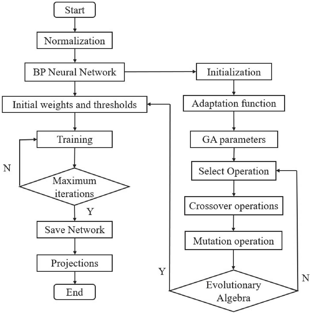
Figure 7 Basic flow of the combined GAGA-BP neural network model.
From the fundamental idea and flow chart of constructing GA-BP combined neural network model, it is shown of the modeling process includes the following steps:
1. Importing the sample set (including training set and test set) and normalizing it under the ensemble method.
2. Synthesize the neural network topology.
3. Encode and populate it initially. The initial randomly chosen priorities and thresholds are extracted from the BP neural network, encoded, and forming the chromosomes in the genetic algorithm.
4. Determine the appropriate fitness function with reference to the objective function.
5. Set the genetic algorithm control parameters. Determine the selection of replication method, crossover method, variation method, crossover and variation probability, population size, maximum number of iterations of the algorithm, etc.
6. Genetic evolution operation. Selection, crossover, mutation.
7. Judgment. Judge whether the population after genetic evolution operation meets the set limits, if it meets the set limits, the genetic algorithm stops running, and then the final generation population is obtained.
8. Fine-tune into BP neural network. Decode the chromosome with the strongest adaptive capacity in the last generation population in the genetic algorithm, replace the best linkage weights and thresholds gained by the genetic algorithm with the respective values selected randomly by the BP neural network model, start the train of BP neural network, and when the set precision or the largest number of generations is reached, the BP neural network training is completed.
9. Simulation prediction. The training network model is used to forecast the results.
4 Data Preprocessing and Implicit Layer Structure Optimization for GA-BP
4.1 Optimization of Sample Data Pre-processing Methods
Neural network training requires normalization of the measured data, i.e., mapping the raw data to a selected normalization interval. Accordingly, the dimensioned raw data can be transformed into a purely numerical scalar, which can effectively prevent trapping in the saturation zone of the human-type transfer function while improving the model training speed and sensitivity [22]. Therefore, the range of the normalization interval has an important impact on the performance of neural network models.
To seek the optimal normalization interval for the GA-BP neural network model, the Postreg function in the MATLAB neural network toolbox was used to carry out regression analysis to verify the training effect of the model that takes different normalization intervals for normalization [23]. The education high-quality of every normalization interval is characterized via the correlation parameter (i.e., the correlation coefficient between the community output and the goal output), the place the nearer the R fee is to 1, the nearer the community output is to the goal output, and the higher the overall performance of the network, as proven in Figure 8. As can be considered from the figure, the education impact of the community mannequin the use of specific normalization intervals is discrete, and the pleasant normalization interval is [0.05, 0.95].

Figure 8 Training effect of network with different normalized intervals.
4.2 Implicit Layer Structure Optimization
The structure of the infant and output layers of the neural network model is decided by both the learning samples of the predicted object and the demand results, and thus the composition of the intermediate implicit layers and the number of neuron nodes they contain will directly affect the learning ability and the level of computational processing of the model. It should be noted that too few nodes will cause poor fault tolerance of the model, resulting in a reduced ability to identify training samples. In contrast, too many nodes cause a significant increase in the running time of the learning algorithm and reduce the value of practical engineering applications [24]. Therefore, the implicit layer structure of the model needs to be adjusted appropriately according to the specific situation.
(a) Single implicit layer and number of neurons
The relationship between the number of neurons in the implicit layer and the number of neurons in the inflow layer is shown in Figure 9.
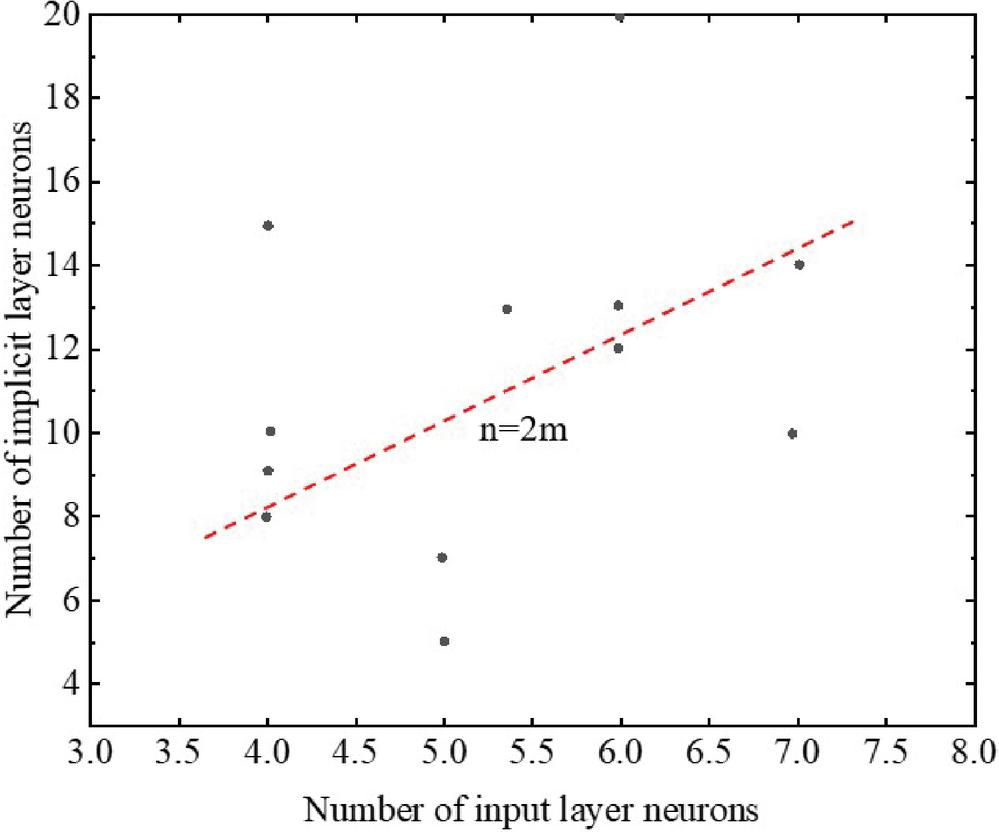
Figure 9 Relationship between the number of neurons in the hidden layer and the number of neurons in the input layer.
Using the least squares technique to curve healthy the above data, the relationship between the best range of neurons in the single hidden layer and the variety of toddler neurons can be obtained, and it can be viewed that the most efficient interval of the quantity of nodes in the single hidden layer is [4, 7]. The range of nodes that can be protected in the single hidden layer is confined with the aid of the model itself, and it is apparent that it can’t meet the working prerequisites with a excessive variety of toddler neurons.
(b) Double hidden layer and number of neurons
When using the measured data as training samples for the prediction model, i.e., when the number of input neurons is large, the single hidden layer structure will significantly reduce the network training effect and model prediction accuracy due to the excessive number of neurons included [25].
The single and double hidden layer training of GA-BP neural network was carried out separately with reference to the relevant methods and data, and the training effects are shown in Figure 10.
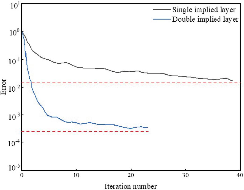
Figure 10 Single- and double-implicit layer training effect.
From Figure 10, it can be shown that the numbers of cycle iterations to reach the expected target error are all smaller for the double-implicit layer structure than for the single-implicit layer structure, suggesting that the neural network pattern with the double-implicit layer structure is much better trained than the single-implicit layer structure when the number of nodes in the input layer is larger.
Part of the training procedure code is as follows:
[Pn, minp, maxp, Tn, mint, maxt] premnmx (P, T);
[kn, ks] mapminmax (k);
[fn, fs] mapminmax (f);
p Pn; t Tn;
net newff (minmax (P), [a, b], {‘tansig’, ‘purelin’});
net. train Param. show ;
net. train Param. epochs ;
net. train Param. goal ;
net. train Param. lr ;
[net, tr] = train (net, Pn, Tn); p, t.
where P and T are the input and output of the training samples after sample normalization, and , are all the just-in-time adjustment parameters.
5 Deep Foundation Pit Deformation Prediction Based on Optimized GA-BP Neural Network
The depth of a subway project is 11 m, using double-row pile support method, and the values of soil mechanical parameters are measured by the laboratory in the range of kPa, , kPa, excavation state is cantilever excavation state, and the values of six points at 2 m, 2.5 m, 3 m, 3.5 m, 4 m and 5 m are taken for Displacement inverse analysis.
5.1 The Process of Implementing Neural Networks
The number of neurons in the input level generally depends on the number of sample attributes. In the deep foundation pit deformation prediction model, the sample attributes are input to the neurons in the input level, passed to the hidden level, and then output by the output level. In deep foundation pit deformation prediction, the sample attributes refer to the monitoring data of each monitoring item or the factors affecting the pit deformation [26].
When monitoring data are used as input data, the purpose of better utilize the regularity between data, the input data cannot be processed in parallel, i.e., the data are all input at once, and the relationship between time and data should be fully considered. Historical monitoring deformation data has a certain guiding effect on the prediction of future data, so the data can be processed by the method of time series, and the data can be cyclically crossed to make the data more rational. Taking the surface settlement deformation as an example, the sequence consisting of data of equal time intervals is , and the deformation is predicted for several future periods.
When the sample data are input into the model, because the data have different magnitudes and physical meanings, direct input may lead to large prediction errors in the model due to large data gaps, which affects the operation results. Therefore, it is essential to standardize the data in order to convert the sample data into dimensionless quantities transformed between [0, 1] or [1, 1]. The actual formula is as following:
| (22) |
In the above equation, x is the initial sample data, and are the largest and smallest values of the original sample data, and y is the normalized sample data. After normalization, Equation (22) is reverse normalized in to obtain the practical value of the output metric in the output data.
| (23) |
The size of the initial population should be determined according to the actual problem. If the size is too large, the search efficiency decreases; if the size is too small, it may produce no solution. Generally, N is taken between 20 and 100. The fitness function is determined by the final learning error after training, and the error formula is
| (24) |
The final search result of the genetic algorithm is to obtain the weights and thresholds corresponding to the minimum sum of error squares, but the whole evolutionary process is oriented to increase the fitness function of individuals, so the fitness feature is expressed as the reciprocal of the sum of error squares.
| (25) |
where is the error sum of squares, is the number of output nodes, the desired output value, the actual output value, and the fitness function.
The crossover operation is a crucial part of the genetic algorithm, which exchanges some of the genes of two parent individuals to form a new individual, which inherits some of the characteristics of the parent [27]. Also, it is a means to obtain new individuals. The larger the crossover probability, the faster the convergence to the optimal solution range, but too large a crossover probability makes the model converge to a particular solution and the subsequent optimization search operation cannot be performed. The choice of the crossover method is closely related to the encoding method, and the procedure of this paper uses real number encoding for the operation, and the specific crossover operation is as follows.
The crossover of the kth chromosome and the lth chromosome at position :
| (26) | ||
| (27) |
where is a random number between [0, 1].
Mutation refers to changing a value of a gene segment by a set probability for an individual selected in advance, although it also produces new individuals, unlike the crossover operation. The probability of variation is generally between 0.001 and 0.1. If the variation probability is too large, the whole process oscillates; if the variation probability is too small, it is difficult to search for the optimal solution.
The variation of the jth gene of the ith individual, the specific mutation operation is as follows:
| (28) |
where is the lower bound of gene and is the upper bound of gene ; is the random number, is the number of iterations, and the maximum number of evolutions.
5.2 Optimization of GA-BP Neural Network Parameters Determination
The number of iterations with the smallest error was selected based on the initial setting of population size of 50, probability of crossover of 0.8, and probability of variation of 0.1. The preliminary outcomes of the neural network model are illustrated in Table 1. From Table 1, we can get that the mean square error is minimized when the number of iterations is 25. Thus, the number of iterations of the neural network model was fixed to 25. At this time, the highest prediction accuracy is achieved.
Table 1 Mean square error values corresponding to different numbers of iterations
| Iteration Number | Iteration Number | Iteration Number | Iteration Number |
| 5 | 0.0132 | 18 | 0.0103 |
| 6 | 0.0135 | 19 | 0.0107 |
| 7 | 0.0157 | 20 | 0.0102 |
| 8 | 0.0114 | 21 | 0.0126 |
| 9 | 0.0113 | 22 | 0.0108 |
| 10 | 0.0114 | 23 | 0.0107 |
| 11 | 0.0116 | 24 | 0.0101 |
| 12 | 0.0117 | 25 | 0.0094 |
| 13 | 0.0154 | 26 | 0.0132 |
| 14 | 0.0112 | 27 | 0.0134 |
| 15 | 0.0134 | 28 | 0.0115 |
| 16 | 0.0139 | 29 | 0.0117 |
| 17 | 0.0107 | 30 | 0.0098 |
The population size was changed based on the initial determination of the number of iterations as 25, the crossover probability as 0.8 and the variation probability as 0.1. The calculation results of the neural network model are shown in Table 2 below, and when the population size is 50, the calculation results are stable and the error is small.
Table 2 Mean square error values for different population sizes
| Stock Size | Iteration Number | Stock Size | Iteration Number |
| 40 | 0.0124 | 48 | 0.0099 |
| 41 | 0.0098 | 49 | 0.0102 |
| 42 | 0.0175 | 50 | 0.0094 |
| 43 | 0.0112 | 51 | 0.0152 |
| 44 | 0.0164 | 52 | 0.0134 |
| 45 | 0.0109 | 53 | 0.0145 |
| 46 | 0.0099 | 54 | 0.0141 |
| 47 | 0.0107 | 55 | 0.0152 |
5.3 Model Optimization Effect Validation and Displacement Prediction Analysis
To verify the optimization effect of the GA-BP model, the prediction results of the optimized GA-BP neural network were compared and analyzed with the unimproved BP and GA-BP neural network models to characterize the prediction superiority by relative error. The results are shown in Figure 11:
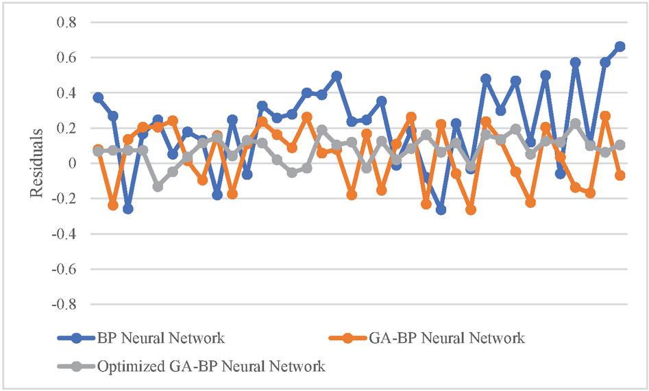
Figure 11 Comparison of model prediction effects.
As can be shown in Figure 11, the residual results of the optimized GA-BP neural network model and its volatility are obviously better than those of the traditional BP model and the GA-BP model without optimization treatment, which further verifies that the model in this article has better forecast accuracy and reliability.
The variation curves of horizontal displacement with time at different depths of CX-6 inclined pipe are shown in Figure 12. From the figure, it can be seen that the overall displacement grows with time in three stages, i.e., fast growth stage I, stable development stage II, and slow deformation stage III. The amplitude of deformation is inversely proportional to the depth of the diagonal measurement; the growth rate of diagonal deformation gradually tends to moderate, and basically remains stable after 50 d.
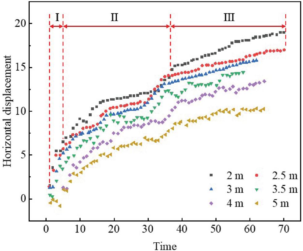
Figure 12 Curve of horizontal displacement at different depths with time.
After repeated trial runs to determine the optimal number of neurons interval of single hidden layer is [4, 7], at this time the model cycle converges fast, the running error is small, and the prediction accuracy is high.
Error analysis was carried out on the predicted value through the precision evaluation index to evaluate the prediction effect. The horizontal displacement error at different depths is shown in Figure 13. As can be seen from Figure 13, on the whole, the deviation of predicted displacement values of each depth is kept within 0.2 mm, and the width of the absolute error interval is 0.07 mm. The maximum relative error is 1.35% at 4.0 m depth, which obviously meets the requirements of construction safety and can provide an accurate reference for engineering construction.
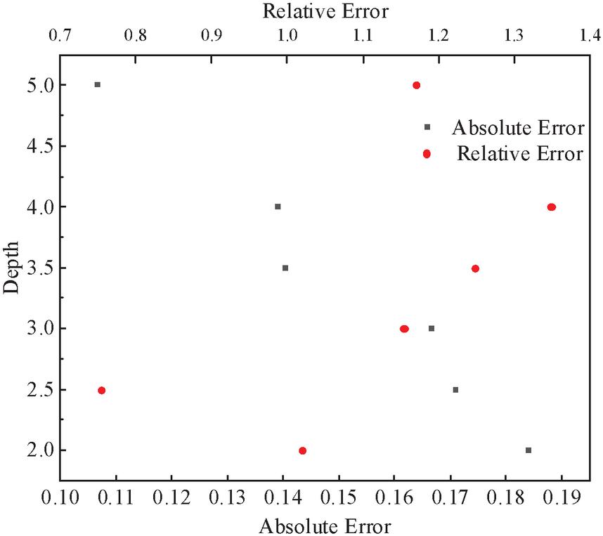
Figure 13 Error analysis of horizontal displacement prediction at different depths.
Table 3 Inversion table of mechanical parameters
| Observation | Measured | Inversion of Mechanical Parameters | Displacement | |||
| Point | Value | Inverse Analysis | ||||
| 2 | 18.63 | 2569 | 0.41 | 14.63 | 22 | 18.69 |
| 2.5 | 16.02 | 16.21 | ||||
| 3 | 14.69 | 14.79 | ||||
| 3.5 | 13.21 | 13.32 | ||||
| 4 | 11.36 | 11.51 | ||||
| 5 | 8.93 | 8.99 |
The displacement observations at 2 m, 2.5 m, 3 m, 3.5 m, 4 m, and 5 m are input to the network, and the mapping relationship is used to find the values of the soil mechanical parameters at the two points. Since the parameter values are dimensionless and normalized at this point, it is necessary to inverse standardize the parameter values to find out the mechanical parameters. It is necessary to inverse standardize the parameter values to find the actual values of soil mechanics parameters, and the specific results are shown in Table 3.
6 Conclusion
The construction business in China is booming, and the deep foundation pit and its surrounding buildings and ground surface will inevitably deform, once the deformation is too large may lead to the collapse of the building and the destruction of the foundation pit enclosure structure, which will cause incalculable economic losses. In this paper, based on the limit equilibrium theory, the method of inverse analysis of deep foundation pit displacement is adopted to determine the mechanical property parameters of soil body by optimizing GA-BP neural network. The specific conclusions are as follows:
(1) The deformation mechanisms of deep foundation pits are summarized as the deformation of the enclosure structure, the settlement of the surrounding ground surface and the uplift of the bottom of the pit. The damage modes of foundation pit slopes are summarized, and their lateral geotechnical pressure calculation methods are compiled according to the specifications.
(2) The working principle of neural network is described. On the basis of BP neural network error back propagation algorithm, this paper adopts genetic algorithm to initialize the initial weights and thresholds of BP neural network, find the interval where the optimal solution exists, and establish the GA-BP combined deformation prediction model.
(3) The GA-BP neural network model is optimized in terms of data preprocessing and hidden layer structure. The correlation coefficient regression analysis verifies that the optimal normalization interval for sample preprocessing is [0.05, 0.95]; the optimal interval for the number of neurons of single hidden layer is [4, 7], and the double hidden layer structure is suitable for the case of more number of input neurons, which can add monitoring data in real time as needed to prevent function overflow and help improve the speed and accuracy of prediction results.
(4) Combined with a subway project, comparing the prediction results of three models, the residual values and volatility of the optimized GA-BP neural network model proposed in this paper have obvious superiority. The foundation pit displacement grows with time in 3 stages, such as fast growth, stable development and slow deformation, and the deformation trend has time memory; with the help of displacement inverse analysis results, the mechanical parameters , , and are inverted using the mapping relationship.
In this paper, the number of nodes in the hidden layer of the BP network training parameters is selected only through repeated experiments to obtain a relatively accurate result, and further theoretical research and exploration are needed for the selection of the number of nodes. At present, only the GA-BP neural network model is designed with a double-implicit layer structure, and the possibility of using a three- or four-implicit layer structure is to be further studied to improve the computational speed and prediction accuracy of the neural network model.
References
[1] Peng K, Zhou Y, Liu Y, et al. The Application of Improved Genetic Algorithm to the Back Analysis of Foundation Pit Construction[C]//IOP Conference Series: Earth and Environmental Science. IOP Publishing, 2021, 676(1): 012124.
[2] Tan Rujiao, Xu Tianhua, Xu Wenjie, et al. Neural network-based inversion of soil parameters for large deep foundation pit projects[J]. Journal of Hydropower, 2015, 34(7): 109–117.
[3] Shen S.C., Chang Q.C., Lan Y., et al. Analysis of spatial and temporal effects of deep foundation pits based on evolutionary neural networks[J]. Journal of Rock Mechanics and Engineering, 2005, 24(A02): 5400–5404.
[4] Xue X, Zheng Y, Wang X. Prediction Method of Heavy Load Wheel/Rail Wear Mechanical Properties Based on GA-BP Hybrid Algorithm[J]. European Journal of Computational Mechanics, 2022: 409–432.
[5] Li YJ, Xue YD, Yue L, et al. Deep foundation pit deformation prediction based on genetic algorithm-BP neural network[J]. Journal of Underground Space and Engineering, 2015 (S2): 741–749.
[6] Daneshkhah E, Nedoushan R J, Shahgholian D, et al. Cost-effective method of optimization of stacking sequences in the cylindrical composite shells using genetic algorithm[J]. European Journal of Computational Mechanics, 2020: 115–138.
[7] Song Chuping. An improved BP neural network method for deep foundation pit deformation prediction [J]. Journal of Civil Engineering and Management, 2019, 36(5): 45–49.
[8] Kalanad A, Rao B N. Edge-crack diagnosis using improved two-dimensional cracked finite element and micro genetic algorithm[J]. European Journal of Computational Mechanics, 2013, 22(5–6): 254–283.
[9] Zhou D, Wu H, Mai J, et al. The Research on Distributed Parallel Optimal Design System of Foundation Pit Engineering[C]//2010 International Conference on Computational Intelligence and Software Engineering. IEEE, 2010: 1–4.
[10] Wang Zhaoxin. Application of neural network based on genetic algorithm in deep foundation pit deformation prediction [D]. Shijiazhuang College of Economics, 2015.
[11] Clough G W. Construction Induced Movements of Insitu Wall, Design and Performance of Earth Retaining Structure[C]//ASCE. 1990: 439–479.
[12] Xu W, Feng J S. Parameter Optimization Design of Soil Nail Supporting to Deep Foundation Pits[C]//Advanced Materials Research. Trans Tech Publications Ltd, 2013, 671: 235–239.
[13] Liu C Y, Wang Y, Hu X M, et al. Application of GA-BP neural network optimized by Grey Verhulst model around settlement prediction of foundation pit[J]. Geofluids, 2021, 2021: 1–16.
[14] Taoshen L. Co-evolutionary Algorithm and It’s Application for Retaining and Protecting Engineering of Foundation Pits[J]. Journal of Computer Aided Design and Computer Graphics, 2004, 16(4): 523–529.
[15] Yang Z, Dong X, Xie D, et al. Research on Optimal Design of Foundation Pit Anchor Support based on Improved Particle Swarm Optimization[C]//IOP Conference Series: Earth and Environmental Science. IOP Publishing, 2019, 300(2): 022063.
[16] Zhou D, Wu H, Mai J, et al. Decompose-Collaborated Evolution Optimum Design of Foundation Pit Engineering[C]//2010 International Conference on Artificial Intelligence and Computational Intelligence. IEEE, 2010, 3: 64–69.
[17] Zhao S L, Liu Y. Displacement back analysis on supporting structure of deep foundation pit based on evolutionary neural nrtwork[C]//2009 International Conference on Wavelet Analysis and Pattern Recognition. IEEE, 2009: 171–174.
[18] Chen Qiu-Lian, Li Tao-Shen, Wu Heng, et al. Genetic algorithm-based collaborative evolutionary processing model for foundation pit support[J]. Computer Applications, 2004, 24(10): 139–140.
[19] Grégoire D, Maigre H, Morestin F. New experimental techniques for dynamic crack localization[J]. European Journal of Computational Mechanics/Revue Européenne de Mécanique Numérique, 2009, 18(3–4): 255–283.
[20] Liu YJ, Li CM, Zhang JL, et al. Genetic-neural network-based real-time prediction method for deep foundation pit deformation[J]. Journal of Rock Mechanics and Engineering, 2004, 23(6): 1010–1014.
[21] Yi, Huangzhi. Optimization of GA-BP model in predicting the deformation of subway station pit project[D]. Hefei University of Technology, 2020.
[22] Song Q, Zhang J J, Liu Y S. Study on Displacement Prediction Model of Foundation Pit[C]//Advanced Materials Research. Trans Tech Publications Ltd, 2014, 834: 679–682.
[23] Liu J, Li FH, Liu XX. Optimization of GA-BP neural network model and foundation pit deformation prediction [J].
[24] Yuhao L, Xiao F. Research on Prediction of Ground Settlement of Deep Foundation Pit Based on Improved PSO-BP Neural Network[C]//E3S Web of Conferences. EDP Sciences, 2021, 276: 01014.
[25] Xu Hongquan, Luo Hailiang, Li Chunsheng, et al. Design optimization of deep foundation pit pile-anchor support structure based on genetic algorithm and MATLAB implementation[J]. Highway Engineering, 2012 (3): 158–161.
[26] Bu K Z, Zhao Y, Zheng X C. Optimization design for foundation pit above metro tunnel based on NSGA2 genetic algorithm[J]. J Railw Sci Eng, 2021, 18(2): 459–467.
[27] Mwangi A D, Jianhua Z, Gang H, et al. Ultimate pit limit optimization methods in open pit mines: A review[J]. Journal of Mining Science, 2020, 56: 588–602.
Biographies

Guo Yunhong obtained a Bachelor of Science degree from Henan Normal University in 1997, and a Master of Engineering degree from Beijing University of Posts and Telecommunications in 2006, currently serves as an associate professor in the Railway Engineering School of Zhengzhou Railway Vocational and Technical College. His research fields and directions include computer application technology, network and security, project management and engineering applications.

Zhang Shihao obtained a bachelor’s degree in engineering from Liaoning University of Science and Technology in 2016, and a Master of Engineering degree in engineering from Chang’an University in 2019, currently works as an assistant teacher in the Railway Engineering School of Zhengzhou Railway Vocational and Technical College. His research fields and directions include subgrade and pavement, road disaster prediction and treatment, and new materials for construction engineering.
European Journal of Computational Mechanics, Vol. 32_1, 53–84.
doi: 10.13052/ejcm2642-2085.3213
© 2023 River Publishers