Slope Stability Analysis Based on the Coupling of SA and Limit Equilibrium Mechanics
Guo Yunhong* and Zhao Liang
Railway Engineering College, Zhengzhou Railway Vocational & Technical College, Zhengzhou 450052, China
E-mail: xscgyh@163.com
*Corresponding Author
Received 29 April 2023; Accepted 28 May 2023; Publication 11 July 2023
Abstract
The limit equilibrium strip method of slope has become mature, but because of the complexity of slope instability with many degrees of freedom and high nonlinear, a more three-dimensional and mature method is needed for slope problems. Based on the overall force balance and moment balance of slope, a unified model of three dimensional limit balance methods is established in this paper. Given different assumptions, the analytical expressions of each traditional model are obtained to avoid the problem of difficult boundary treatment when the original method is divided into bars and columns. The influence of the trailing edge point B and shear outlet A on the central axis of the sliding body, and the control arc radius variable t on the calculated value of the three-dimensional slope stability coefficient is discussed in detail. Then, based on the simulated annealing algorithm, the state generating function, state accepting function and temperature updating function are constructed, and the calculation method of optimizing the sliding surface search of the slope by using the simulated annealing algorithm is proposed, and the stability analysis of the slope of a hydropower reservoir dam area in Guangxi is carried out. The results show that the position of the sliding surface obtained by searching around the design value K 1.10 is basically consistent with the actual one, which proves that the mechanical analysis method of coupling SA and limit equilibrium is convenient and efficient in the slope stability analysis.
Keywords: Mechanical calculation, SA, optimization problem, limit equilibrium, slope stability calculation.
1 Introduction
Slope stability analysis is one of the important research topics in geotechnical engineering, its research methods include: limit equilibrium method, limit analysis method, numerical analysis method, etc. Among them, the limit equilibrium method is the most widely used, but it must rely on the experience of researchers to try to calculate a series of sliding surfaces to find the minimum safety factor and the corresponding critical sliding surface position [1, 2]. As shown in Figure 1, the following figure shows the general treatment of roadbed slope and the arrangement of monitoring instruments.

Figure 1 Construction and monitoring methods of roadbed slope.
Firstly, as an important part of rock mass mechanics, the research progress of slope stability is closely related to the urgent need of human engineering activities and the rapid development of related disciplines. The early research is based on the simple homogeneous elastic and elastoplastic theory of semi-empirical and semi-theoretical slope analysis method, the calculation results are very different from the actual engineering situation. By the early 1960s, the expansion of the scale of engineering construction led to the slope problems became increasingly prominent. Especially after a series of engineering accidents such as the Vaiont reservoir landslide in Italy in 1963, people began to deeply study the stability of rock slope. The realization that geological analysis and mechanical mechanism analysis must be closely combined led to the rigid body limit equilibrium method. In latest years, many students have dedicated themselves to the lookup of the vital slip floor computerized search technology, proposing a range of relevant to the arc slip floor or non-arc slip floors search methods, such as the Monte Carlo approach and finite factor combination, criticality method, genetic evolutionary algorithm, sample search method, stumble upon ant colony algorithm, neural community, and more than one regression, etc. Compared with the exhaustive technique and dichotomous approach used in the early days, the accuracy and convergence of the above strategies have extended a lot, which has performed a fine function in slope balance lookup and realistic engineering applications, however from time to time it additionally takes place that the calculation outcomes are no longer the excessive fee of the universal security aspect. Common secondary side slopes are shown in Figure 2.
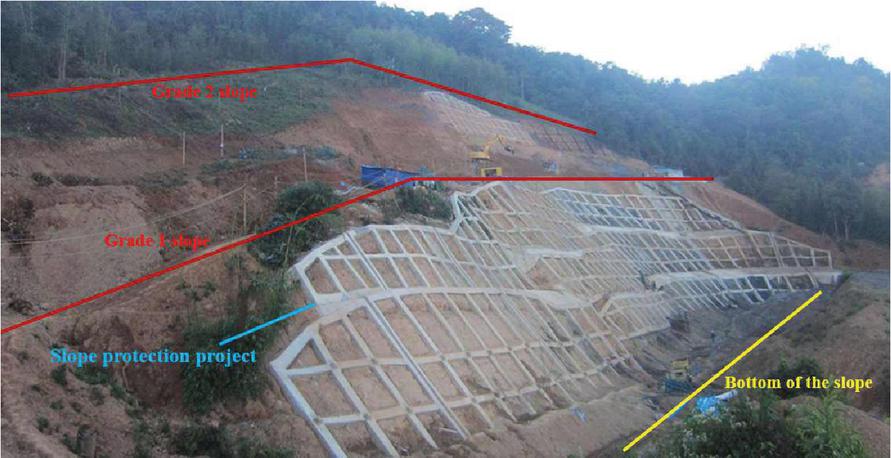
Figure 2 Schematic diagram of the secondary slope.
The simulated annealing algorithm (SA) originates from statistical physics, which simulates the bodily manner from gradual cooling to the ultimate crystallization of an object in the molten state. The simulated annealing algorithm takes benefit of the similarity between the answering system of the trouble and the annealing method of the melting object and makes use of a random simulation of the annealing system of the object to entire the answer of the problem, that is, the price of the parameter is adjusted underneath the motion of to managedage parameter (temperature) till the chosen parameter cost sooner or later makes the strength feature attain the world minimal cost [3].
The simulated annealing algorithm has the following traits in contrast with different algorithms:
(1) Accepting the optimized solution with a certain probability The simulated annealing algorithm (SA) differs from the traditional random search method in its search strategy, which introduces no longer solely excellent random factors, but additionally the herbal mechanism of the annealing procedure of the bodily system [4]. The introduction of this natural mechanism makes the simulated annealing algorithm in the iterative process not only accept the target function to become “good” trial points but also with a certain probability to accept the target function value to become “bad” trial points.
(2) Introduction of algorithm control parameters The annealing temperature-like algorithm manipulates parameters, which divides the optimization process into degrees and establishes the trade-off standards of the random states below each stage, and is introduced. The Metropolis algorithm then provides a straightforward mathematical model for the acceptance feature. The simulated annealing algorithm has two key steps: first, at each control parameter, a neighboring random state is generated from the previous iteration point, and second, the acceptance criterion lined by the control parameter determines the trade-off of this new state, forming a specific length of random Markov chain. Second, until the control parameter goes to zero and the state chain stabilizes at the optimal state of the optimization problem, the acceptance criterion is gradually reduced, and the control parameter is gradually increased. Thus improving the reliability of the global optimal solution of the simulated annealing algorithm.
(3) Use of object function values for search Traditional search algorithms no longer solely want to use the cost of the goal function, however additionally frequently want the cost of the by-product of the goal feature and some different auxiliary statistics to decide the search direction, when these statistics no longer exist, the algorithm will fail [5, 6]. The simulated annealing algorithm makes use of solely the fee of the health feature converted through the goal function, it can decide the similar search path and search range, barring different auxiliary information.
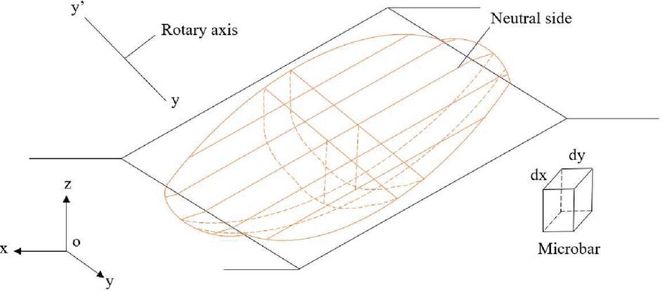
Figure 3 Three-dimensional stability analysis model of slope.
2 Unified Model of Three-Dimensional Limit Mechanical Equilibrium Method for Slopes
2.1 Establishment of a Unified Model
As shown in Figure 3, the x-coords are taken as the main sliding direction, the coords are taken as the slope direction in the vertical sliding direction, and the z-coords are taken as the vertical ascent direction. x, y, and z conform to the right-hand rule, and the microcolumn with x direction as dx and y direction as dy is taken for analysis (shown in Figure 4). The microbar column has six faces, except for the top face, each face is subject to three forces, two shear forces, and one vertical force. N represents the vertical force, and the subscripts indicate the action face, represents the vertical force on the face normal to y [7]. T represents the clipping force, the 1st scale of T represents the surface of action, and the 2nd scale represents the flow direction of the force. represents the shear force in the x direction on the face normal to y and dW represents the volume of the microbar column force.
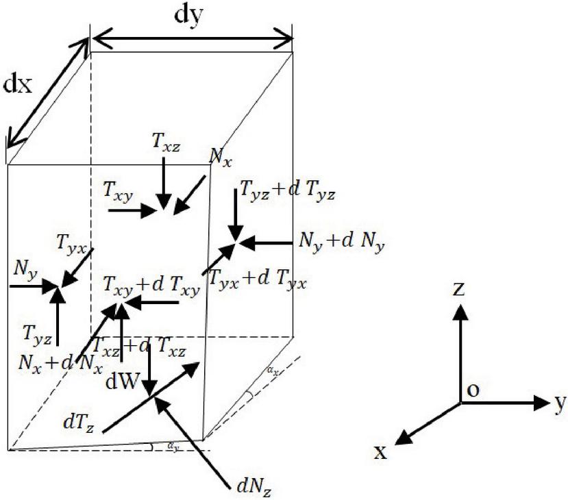
Figure 4 3D microbar column force diagram.
2.1.1 Basic mechanical assumptions
The mechanical model is based on the following assumptions:
(1) The stability factor is the material’s strength discount factor, or the proportion of the shear strength throughout the entire slip fracture surface compared to the actual shear strain produced.
| (1) |
(2) The oil is rigid, and the bottom slip surface obeys the Moore-Coulomb strength damage criterion:
| (2) |
Where, , u is the pore water pressure and is the area of the slip surface at the bottom of the microbar column.
(3) The point of action of the normal force at the bottom of the microbar is at the midpoint of the bottom of the bar.
2.1.2 Mechanics modeling
(1) Unified model of force equilibrium stability coefficient Establish the equilibrium equation of the sliding body as a whole along any linear direction in space (as shown in Figure 5), and introduce Equation (2), then the calculation formula of the force balance stability coefficient can be derived, the specific steps are as follows:
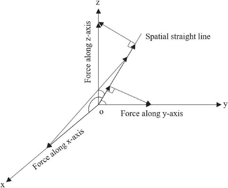
Figure 5 A diagram of the force projection along any plane in space.
Let the direction cosine of a certain line in space be , the direction cosine of dN be , and the direction cosine of dT be , then the equilibrium equation of the overall force along the direction of the line is:
| (3) |
Substituting Equation (2) into (2.1.2), the collation gives:
| (4) |
Where,
| (5) | ||
| (6) |
Equation (4) is the unified calculation model of the stability coefficient derived by static equilibrium [8].
(2) Unified model of moment balance stability coefficient Establish the second stability equation of the sliding physique as a total with any straight line in house as the axis of rotation, and introduce Equation (1), then the calculation formulation of the second stability steadiness coefficient can be derived. The precise steps are as follows.
Let a certain line through a point in space , the direction cosine is , the direction sine is , that is, the line O’D’ in Figure 6. Taking the line as the rotation axis, the forces in the model are first projected along the x, y, and z axes, and the combined forces projected in each direction are then projected in the vertical direction of the rotating line, and their distances (force arms) from the line are , , and (as shown in Figure 6).
As shown in Figure 6, OD is the line passing through the origin and parallel to O’D’, the angles between O’D’ and the x, y, and s axes are , , , respectively, and so is OD; ABC is the plane perpendicular to the line OD; AD, BD and CD are the projections of the combined forces in the model along the x, y and s axes in the perpendicular direction of the line; BC is the angle between BC and the x, y and The angles of BC and x, y and axes are /2, , , the angles of CA and x, y and z axes are , /2, , the angles of AB and x, y and axes are , , /2 respectively.
From Figure 6, it can be seen that BC is the normal to the face AOD, AC is normal to the face BOD, and AB is normal to the face COD [10]. Thus, the vertical distance between the projection of the combined forces in the model along the x, y; axes in the vertical direction of the projection of the spatial line and the rotation axis OD, i.e., the force arms , , , is transformed to the point to the normal to BC, CA The problem of finding the perpendicular distances from the point to the faces AOD, BOD, and COD normal to BC, CA, AB, and all through the point .
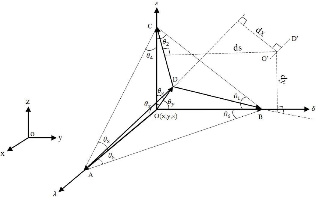
Figure 6 Geometric relationship of the moment force arm.
The directional cosine of BC, CA, and AB is first found, based on the geometric relationship shown in Figure 6:
The directional cosine of CB is:
The directional cosine of AC is:
The directional cosine of AB is:
Then,
| (7) |
Because
| (8) |
So
| (9) |
Take the positive, i.e.
| (10) |
Similarly,
| (11) |
Then the equations of surface AOD, BOD and COD are
| (12) |
Then the equation of the overall moment balance is
| (13) |
Substituting Equation (2) into Equation (2.1.2) and organizing gives
| (14) |
Equation (14) is the unified calculation model of the stability coefficient derived from moment balance [11].
In the three-dimensional limit equilibrium stability analysis of the slope, generally only the overall moment balance of the line around the point and parallel to the y-axis is considered, which can be known in this case.
| (15) | ||
| (16) |
(3) Solution of dN From the above-unified model, it can be seen that the equation contains only two unknown quantities, F and dN. As long as the expression of dN is determined, the calculation of the stability coefficient F can be obtained by iteration.
Because the expressions of dN, in the limit equilibrium method are obtained from the force balance in a certain direction of a single column, the general expressions for solving dN can be deduced by satisfying the force balance in any linear direction along the space by all the forces in the microbar column [11, 12].
Let the direction cosine of a certain line in space be , then the equilibrium equation of the force along the direction of that line for each microbar column is
| (17) |
Substituting Equation (2) into Equation (2.1.2), the collation yields
| (18) |
Where,
| (19) | ||
| (20) | ||
| (21) |
Equation (2.1.2) is the general expression to solve for dNz.
3 SA-based Optimization Method for Mechanical Calculations
Since Kirkpatrick, Gelatt, Jr., and Vecchi posted their seminal papers based totally on the preceding lookups on statistical mechanics, the simulated annealing algorithm has been praised as a “savior” for fixing many hard combinatorial optimization problems [13, 14]. “It has been used in applications such as a computer-aided sketch of very giant scale built-in circuits (VISI), picture processing and pc vision, telecommunications, economics, and many different engineering and scientific fields [15]. It is a general and effective approximation algorithm suitable for solving large-scale combinatorial optimization problems [6]. Combinatorial optimization problem is to solve the optimal value (maximum or minimum value) of the objective function under given constraints. The optimization trouble consists of three fundamental factors.
(1) Variables – the basic parameters selected in the solution process.
(2) constraints – the constraints on the value of the variables.
(3) The objective function is a function that gauges the viability of the proposed solution.
A combinatorial optimization problem illustration can be shown as a dyad (S, f), where the solution pool S is the collection of feasible solutions [17].
The objective function f is a mapping defined as:
| (22) |
The minimization issue, also known as the issue of locating the minimum of the desired function, is symbolized as:
| (23) |
The minimization problem and the maximization problem can be equivalently transformed by changing the sign of the objective function [18].
3.1 Overall Optimal Solution, Neighborhood Structure and Local Optimal Solution for Mechanics Problems
3.1.1 Optimal solution for overall mechanics
Let , be an instance of the combinatorial optimization problem, , if , holds for all call the overall optimal solution of the minimization problem , .
3.1.2 Domain structure
An example of a combinatorial optimization problem would be , in which case a nearby structure is a translation. .
Where denotes the set of all subsets of S. The implication is that for every solution , there is a neighborhood of the set of solutions that are in some sense “adjacent” to i, a neighborhood of the set . Each j S is called a neighboring solution of i.
3.1.3 Optimal solution for local mechanics
Let N be a domain structure and , be an example of a combinatorial optimization issue, then is said to be a locally optimal solution to the minimization problem . That is:
| (24) |
3.2 Local Mechanics Problem Search Algorithm
Local search algorithm is a general approximation algorithm, whose basic rule is to iterate through the neighboring solutions until they are no longer better. Local search method is flexible and can give a good approximate solution [19, 20].
The algorithm of local search algorithm is described as follows: the regional search process begins with a first answer. , and then uses a generator to continuously search for a better solution than I in the neighborhood S, of the solution I (called the current solution), and if a better solution than i is found, it replaces I with this solution to become the current solution and then continues to until the termination condition is satisfied, look for solutions nearby the current one, which is the algorithm’s last answer [21].
3.3 SA-based Mechanical Calculation Method
3.3.1 Mechanical structure and mathematical model of SA
(i) SA mechanical structure The execution strategy of the simulated annealing algorithm consists of the following steps: probe the entire mechanics solution space starting from an arbitrarily selected initial solution, and generate a new mechanics solution by perturbation, use the Mertopolis criterion to determine whether to accept the new solution, and drop the control temperature accordingly. The flowchart of the simulated annealing algorithm is shown in Figure 7.
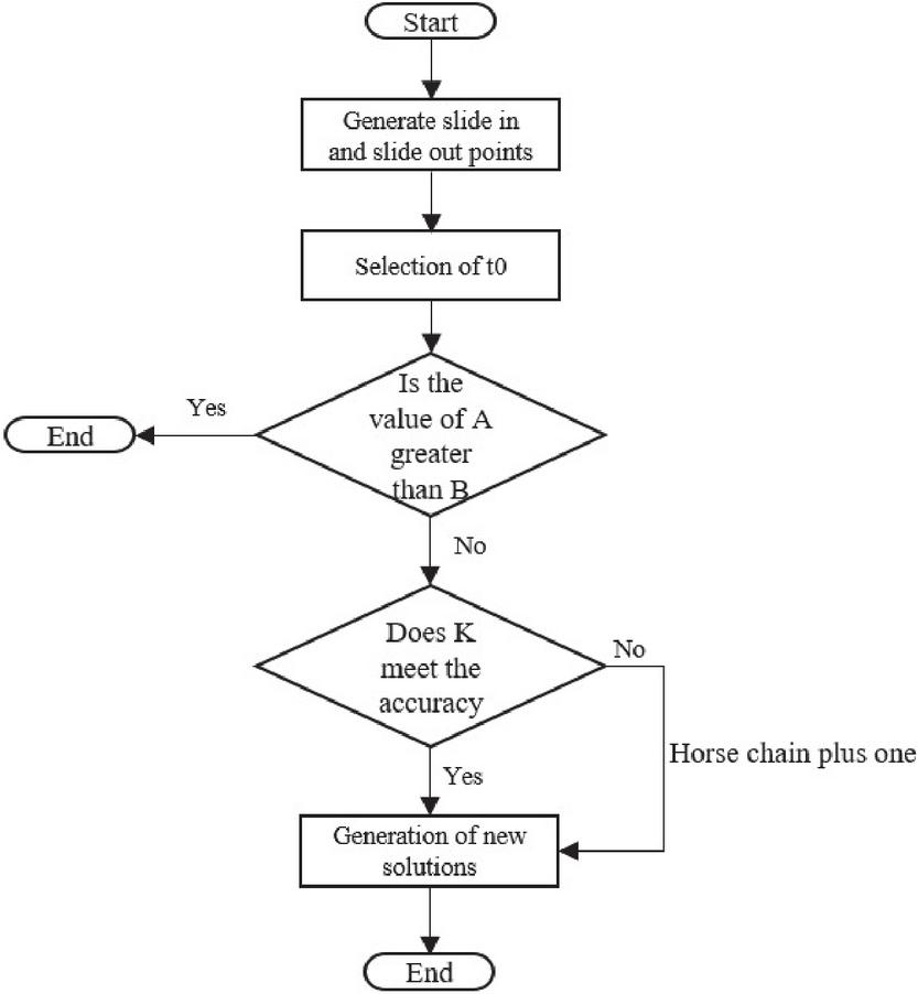
Figure 7 SA flow chart.
(ii) Mechanical model for simulated annealing algorithm The result j is what the algorithm for simulating annealing (SA) visits in the kth iteration, and the probability of the solution j is what the SA visits in the (k+1st) iteration [24]. It consists of two independent probability distributions, the probability of generating solution j from solution i in the kth iteration , where is required to satisfy the normalization condition: , the probability that the solution is accepted , where the kth cycle, the temperature is T, and the expression of the transfer probability for the case i j is as follows.
| (25) |
Since is not always equal to 1, there is a possibility that the new solution will not be accepted and the algorithm stays at solution i with probability:
| (26) |
Since is a kernel set, the random process represented by the random variable generated by the simulated annealing algorithm is a Markov chain whose one-step transfer probability is defined by Equations (25) and (26), and the one-step transfer probability is noted as:
| (27) |
Then the transfer probability for step k is:
| (28) |
Where I is the unit matrix and denotes the temperature value at the tth iteration. The meaning of the matrix is:
| (29) |
That is, the probability of being in state i by m iterations and in state j by the mth kth iteration [25].
(iii) Finite time implementation of SA Solving the international greatest answer is vital trouble in optimization algorithms. When the characteristic is nonconvex or provides segmental continuity, it is tough to clear up the international superior answer the usage of the usual nonlinear programming method, which is a neighborhood search algorithm [26]. For nonsmooth and distinctly pathological optimization problems, gradient-based typical nonlinear programming strategies are additionally frequently powerless. For combinatorial optimization problem, the traditional nonlinear programming method is not effective. In recent years, some direct search methods have been proposed, such as simulated annealing algorithm (SA), mean field annealing algorithm, genetic algorithm and so on. Simulated annealing algorithm is a kind of computation method which has attracted much attention in recent years. It can solve some problems which are difficult to be solved by traditional nonlinear programming methods. It has been widely studied in many fields such as generation scheduling, control engineering, machine learning, neural network, function optimization and so on [27].
The simulated annealing algorithm (SA) is a stochastic search method, which is based totally on statistical thermodynamics and introduces the herbal mechanism of the annealing system of bodily systems. The introduction of this herbal mechanism no longer solely makes the simulated annealing algorithm (SA) receive some higher generation factors in the iterative process, however additionally be given deteriorating options with a sure probability. It takes the principle of finite-state singular Markov chains in stochastic procedures as its mathematical basis, and the acceptance chance decreases regularly as the manage temperature decreases, and this search method can efficaciously make it keep away from falling into nearby minima. And the simulated annealing algorithm (SA) does now not want any auxiliary data (such as gradient information), has no requirement for the goal feature and constraint function, and has robust robustness, international convergence, implied parallelism, and broad applicability. The simulated annealing algorithm (SA) is a vital department of computation in accordance with the legal guidelines of nature, which simulates the optimization hassle with the warmness stability trouble in statistical mechanics and opens up a new way to clear up the international optimization problem. The optimization hassle is comparable to the metallic annealing manner in nature: the goal feature of the optimization trouble is equal to the inner electricity of the metal, the house of the blended states of the variables of the optimization hassle is equal to the interior kingdom house of the metal, and the answer method of the optimization hassle is a search for the blended states to decrease the price of the goal feature.
When the simulated annealing algorithm (SA) solves a global optimization problem, in theory, it is necessary to reach an equilibrium through many iterations for each temperature. When the temperature drops from high enough to low enough, the lowest point of the objective function can be found. For the ideal model, the classical simulated annealing algorithm converges to the global optimal solution under the following conditions: the initial temperature is high enough, the cooling rate is slow enough, and the termination temperature is low enough [28]. However, the number of iterations needed to reach the equilibrium of the objective function value at each temperature is very large, and the ideal annealing process requires the temperature to drop continuously and very slowly, which is difficult to do. They are the main reason for the low efficiency of simulated annealing algorithm (SA).
The determination of the initial temperature, the selection of the cooling function, the determination of the search method, the mechanism of solution generation, and the determination of the ending criterion are all important issues in constructing the simulated annealing algorithm [29]. The finite-time implementation of the simulated annealing algorithm is of great importance both theoretically and in terms of applications.
A series of factors known as the “cooling agenda” is used to modify the algorithm’s system to mimic the asymptotic convergence regime of the simulated annealing process and get the program to approach the ideal solution after a short running method. The cooling agenda includes the initial values of the manipulation parameters, their decay functions, the length of the associated Markov chain, and the halting threshold. It is a significant factor that affects the final result of the fake annealing process, and its careful selection is part of the application’s software’s hidden weapon [30, 31].
(1) Starting point for the control parameter t According to practical evaluation, the algorithmic process should seek the broadest feasible range of solutions in an acceptable amount of time. Since only a large initial value can meet this condition, the initial acceptance rate should be close to 1. By the Metropolis criterion, , it follows that the controlling factor t’s starting point should be high.
(2) Size of the Markov chain The result of one attempt in a Markov chain depends only on the result of the previous attempt and thus has the memory forgetting function. The length of the Markov chain represents the number of transformations produced by the KTH iteration of the Metropolis algorithm. The selection principle of Markov chain length is: on the premise that the attenuation function of the control parameter t has been selected, the probability distribution of the solution on each value of the control parameter should be stable distribution.
By counting the number of changes (some fixed value) that a uniform distribution should tolerate at least, it is possible to determine the number of changes necessary to smooth the distribution at each value of the control parameter. The amount of changes needed to accept a fixed number of changes, however, grows since the acceptance probability of the changes reduces with lowering values of the control factors, and eventually as . For this reason, certain constants can be used to limit the value of l so as not to produce excessively long Markov chains at small values of t.
The finite sequence “l” identifies the range of solution spaces that the algorithmic process examined and the value “l” indicates how many changes were carried out by the algorithmic process in the kth Markov chain. The following is a discussion of the commonly used methods for determining l.
(1) Fixed length Since the size of the solution space of most combinatorial optimization problems increases exponentially with the problem size n, some relationship between l and n can be established to certify the accuracy of the fake annealing algorithm’s eventual result. The exponential model of the relationship is obviously impractical, and therefore typically considered to be a polynomial function of the issue size n. Rirkpatick et al. used a direct specification of . Using a fixed-length L is a simple approach where l is independent of the value of the control parameter t and is a constant that does not vary with the algorithmic process for a given instance of the combinatorial optimization problem.
(2) Control of the number of iteration steps by the percentage of approval to rejection When the cost of the control factor is high, nearly every state is acceptable, and each kingdom occurs with roughly equal frequency. In this instance, the wide variety of technical procedures can be minimized at that modified factor value. As the fee of the manipulated parameter receives regularly smaller, greater, and larger states are rejected. If the variety of iterations at this manipulated parameter price is too small, it might also additionally cease resulting in upfront falling into a close-by final reply. A more intuitive and effective approach is to increase l as the value of the control parameter decreases. One approach that can be implemented is to give an acceptance count indicator i. The Markov chain at that control value for the parameter ends when the acceptance count reaches i, and the control factor value declines.
(3) Decay function of the control parameters The algorithm procedure may undergo more iterations as a result of the slight decay of the control parameters. This is expected to result in more changes, better neighborhood visits, a wider search area for answers, and a better final solution. Of course, this will also require more CPU time. According to the tests, the size of the existing response may be significantly increased without significantly impacting the reasonableness of CPU time, provided that the decay feature is selected correctly.
(4) Stopping criterion The asymptotic convergence property of controlled simulated annealing offers additional light on the fact that the method’s asymptotic approach to the minimal set of possibilities occurs when the cost of the manipulation factor t steadily reduces. It is only allowed to obtain exceptional, highest-quality options when t is “sufficiently small.” Consequently, “sufficiently small” can, to an extent, be employed as a stopping condition in place of “final solution excellence”. One is to let the value of the control parameter t be smaller than some sufficiently small positive number , which directly constitutes the judgment formula for the stopping criterion, and the other is to determine a termination parameter by the decreasing acceptance probability of the algorithmic process with the value of the control parameter, and to terminate the algorithm if the current acceptance rate of the algorithmic process . This is the standard for stopping that Johnson et al. adopted. This approach strikes a balance between the requirements of the best final response and the CPU time required for the ending standard, and it can be projected that the CPU time will be reduced while the final solution quality is still guaranteed as long as the value of is chosen appropriately.
4 Mechanical Application of Simulated Annealing Algorithm in Slope Stability Analysis
The simulated annealing algorithm described in Section three is a classical simulated annealing algorithm, whose fundamental thought is to examine the answer procedure of a sure kind of optimization trouble with the thermal equilibrium hassle in statistical thermodynamics, attempting to simulate the annealing system of high-temperature objects to discover the world most advantageous or almost world most advantageous answer of the optimization problem, even though it can be given inferior options to a restrained extent and soar out of the nearby most appropriate solution, however it nevertheless of course has the following two deficiency factors.
If the cooling process is slow enough, the performance of the obtained solution will be better, but the corresponding convergence rate is too slow.
If the cooling procedure is too fast, it is probable that the international most fulfilling answer will now not be obtained. From the standpoint of the algorithm process, the simulated annealing algorithm consists of three functions (i.e., nation technology function, country acceptance feature, and temperature replace function) and two standards (i.e., internal loop criterion and outer loop criterion), and the format of these hyperlinks will decide the optimization overall performance of the simulated annealing algorithm. In addition, the choice of the initial temperature also has a significant impact on the algorithm. In the following chapter, we will introduce how the parameters of the simulated annealing algorithm and the parameters of the slope stability analysis are related, and how to adjust the size of each parameter so that the calculation can be done accurately and quickly.
4.1 Design of Mechanical State Generation Function in Slope Stability Analysis
The beginning factor of designing the nation era feature (neighborhood function) must be to make certain that the candidate options are spread over the entire answer house as a lot as possible. Generally, the nation technology feature consists of two parts, namely, the way to generate candidate options and the likelihood distribution of the candidate solutions [32]. The former determines the way in which candidate solutions are generated from the current solution, while the latter determines the probability of choosing different states among the candidate solutions generated by the current solution. The generation mode of the candidate solution is determined by the nature of the problem, which is usually generated in a certain probabilistic way in the neighborhood structure of the current state. The neighborhood function and probabilistic mode can be diversified design, in which the probability distribution can be uniform distribution, normal distribution, exponential distribution, Cauchy distribution, etc.
For the analysis of the soil slope problem studied in this paper is shown in Figure 8.
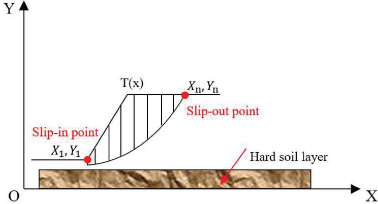
Figure 8 Slope slitting calculation model.
4.1.1 Selection of sliding surface mechanics calculation variables
Assuming that the coordinates of the sliding-in and sliding-out points of the sliding surface are , , now take the points along the X direction from the point with equal spacing , so that we can get , and since are assumed to be known, the unknown variables are . Since the slip-in and slip-out points must be on the soil slope surface, is the design variable. Other quantities are known as long as the to determine the location of the sliding surface, such a selection of design variables can control the number of sub-strip to determine the number of unknown purposes, to get a smooth sliding curve needs to be divided into how many strips of soil, according to the specific engineering situation to determine, but It is not better to divide the sliding surface into more strips, but the calculation time also increases, and it is difficult to reach the specified length of the martensite chain, resulting in slow convergence. The present simulation example is to determine the relationship between the slope length of 28 meters at the bottom elevation angle of 25 and the convergence of the calculation time [33].
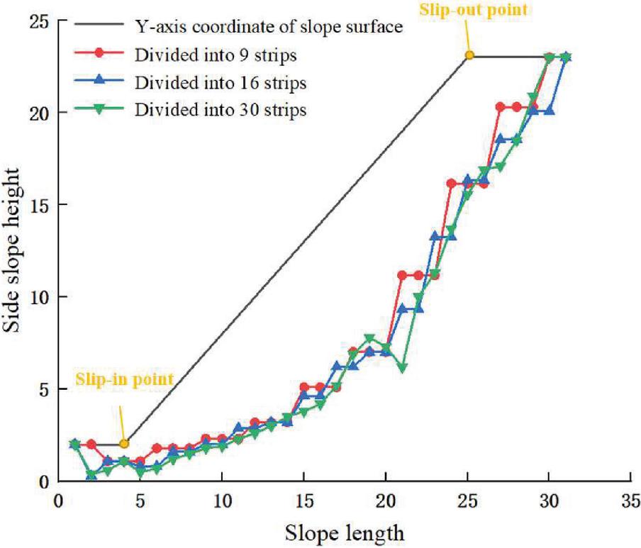
Figure 9 Coordinate diagram of sliding surface with different slits.
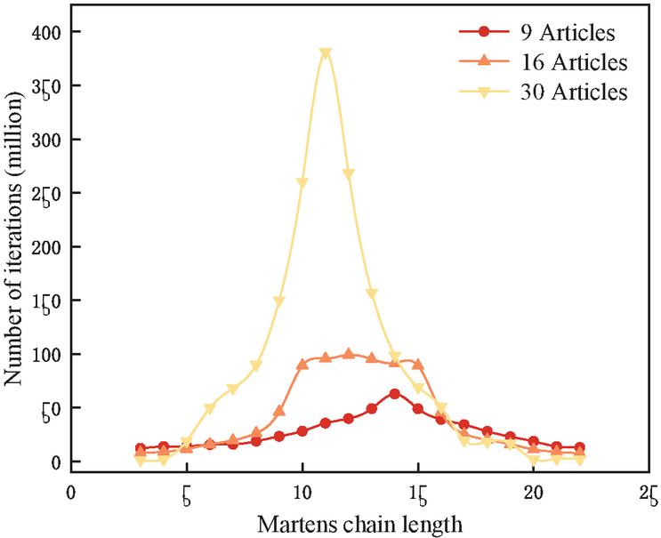
Figure 10 Graph of the number of iterations for calculating the safety factor.
From Figures 8 and 9, it can be concluded that in the case of the slope bottom elevation angle of 25, the calculation speed is relatively fastest when divided into 9 strips, but the sliding surface obtained is the least smooth, which is caused by too few strips and insufficient data calculation, and the calculation speed drops a lot when divided into 30 strips, which is about 4.5 times of 16 strips, and the time of each run is different, which is very different. In the fourth run of the program, the phenomenon that the calculation time was too long and the program could not be jumped out occurred, and it can be concluded from Figure 8 that there are obvious slip resistance points on the sliding surface curve obtained by dividing into 30 strips, which is also an unreasonable factor. calculation method. In other cases where the elevation angle of the slope bottom and other parameters are determined, the above method can also be adapted to determine the number of sliding bars, to achieve the condition that both the calculation speed and smoothness are satisfied.
4.1.2 Selection of mechanical objective function
To obtain the minimum stability safety coefficient K of the slope and the corresponding real most dangerous slip crack surface as the target of this paper, thus K can be taken as the objective function, which is required for optimal numerical analysis.
| (30) |
Where K is the safety factor for the Janbu bar splitting method:
| (31) |
Where:
– horizontal thrust between soil strips.
W – Self-weight of the soil strip.
U – permeable water pressure at the bottom of the soil strip
f – Friction coefficient at the bottom of the soil strip.
c – The cohesive force of the soil.
Since both sides of the equation contain the objective function K, it needs to be calculated by falling generation. Janbu strip method can be applied to sliding surface of arbitrary shape, and the actual engineering cases match well, so the objective function is selected based on the safety factor K of Janbu strip method.
4.1.3 Generation of new sliding surface
Firstly, the possible position intervals of the slip-in and slip-out points are estimated, and their corresponding X-coordinates are . Based on the fact that the slip-in and slip-out points must be on the surface of the soil slope, the corresponding Y-coordinates can also be determined, which are noted as , and then the new solution generation equation can be expressed as:
| (32) | ||
| (33) | ||
| (34) |
Where is a random number between 0 and 1 generated randomly by the computer.
4.1.4 Determination of slope constraints
The slip crack surface formed by the design variables must be within the basic possible range of the slip crack surface determined by the shape and geological conditions of the slope. Specifically, it means that and must not go beyond the outermost left and right sides of the slope surface, while must not go beyond the slope top curve upward and the hard soil surface curve downward, i.e.
| (35) | |
| (36) | |
| (37) |
4.2 Design of Mechanics State Acceptance Function
The state acceptance function is generally given in the form of probability, and the difference between different acceptance functions mainly lies in the different forms of acceptance probability. To design the state acceptance probability, the following principles should be followed.
(1) At a fixed temperature t, the probability of accepting a candidate solution that makes the value of the objective function decrease is greater than the probability of accepting a candidate solution that makes the value of the objective function increase.
(2) As the temperature decreases, the probability of accepting a solution that increases the value of the objective function decreases.
(3) When the temperature tends to zero, only solutions with decreasing values of the objective function can be accepted.
The introduction of the state acceptance function is the most critical factor for the simulated annealing algorithm to achieve global search, but experiments show that the specific form of the state acceptance function does not have a significant impact on the performance of the algorithm. Therefore, the Metropolis criterion is usually used as the state acceptance function in the simulated annealing algorithm.
4.3 Acceptance Criteria for New Solutions
To decide whether to embrace the new solution in this chapter, the enlarged Metropolis admission rule is used. The new approach is accepted if it is workable and superior to the current one; otherwise, the new solution is accepted with the probability of . That is:
| (38) | ||
| (39) |
5 Conclusion
In this paper, based on the unified model of the three-dimensional limit equilibrium method of the slope, the three-dimensional slope parameter backcalculation and excess sliding force calculation formulas are proposed. The modern intelligent optimization method is also applied to the search of the 3D critical sliding surface of the slope to solve this complex problem with multiple degrees of freedom and high nonlinearity. Through the work of this paper, the following conclusions are obtained:
1. Based on the overall force balance and torque balance of sliding body, a unified model of three dimensional limit balance methods is established. Through this model, the expression of unknown quantity dNz in the bottom of sliding surface is determined under different assumptions. The analytical expressions of each traditional model can be obtained, which avoids the problems of boundary processing and column number determination in column division of existing methods. This makes the concrete implementation of various methods, programming becomes more convenient, more simple calculation, improve the efficiency of computing. The three-dimensional Sarma method established in this paper is also improved to make the shear force direction of the bottom sliding surface related to the bottom sliding surface inclination, and the model is fully analyzed.
2. By setting up the country-producing function, country accepting feature, and temperature updating characteristic of the simulated annealing algorithm. This chapter proposes a calculation technique to optimize the search of the sliding floor through the use of simulated annealing algorithm, and via the steadiness evaluation of the slope of a hydropower reservoir in Guangxi, the calculation results are equal to the thrust value calculated by the unbalanced thrust method. And the design value K 1.10 is searched to get. The position of the sliding surface is consistent with the shape of the sliding surface and its position obtained from the actual geological exploration, which indicates that the simulated annealing algorithm is feasible and efficient in the slope stability analysis.
References
[1] Huang Lin. Dynamic Stability analysis of stratified soil slope under earthquake [D]. Southwest Jiaotong University, 2017.
[2] Song J, Wu K, Feng T, et al. Coupled seismic analysis of permanent deformation of shallow and deep failure surface of slope [J]. Engineering Geology, 2020, 274: 105688.
[3] Ai Hui, Wu Honggang, Feng Wenqiang, et al. Shaking table test on deformation and failure mechanism of multi-sliding surface landslide [J]. Journal of Disaster Prevention and Mitigation Engineering, 2018, 38(1): 65–71.
[4] Messai A, Belounar L, Merzouki T. Static and free vibration of plates with a strain based brick element[J]. European Journal of Computational Mechanics, 2018: 1–21.
[5] Gholami M, Hassani A, Mousavi S S, et al. Bending analysis of anisotropic functionally graded plates based on three-dimensional elasticity[J]. European Journal of Computational Mechanics, 2019: 1–25.
[6] Zhang Junwen, Zou Ye, Li Yulin. Failure mode and stability of large multilayer accumulations [J]. Chinese Journal of Rock Mechanics and Engineering, 2016, 35(12): 2479–2489.
[7] Yang Tao, Zhang Zhongping, Ma Huimin. Stability analysis and support selection of multi-story complex landslide [J]. Chinese Journal of Rock Mechanics and Engineering, 2007 (s2): 4189–4194.
[8] Murdock J R, Yang S L. Hydrodynamic stability and turbulent transition with the Vreman LES SGS and a modified lattice Boltzmann equation[J]. European Journal of Computational Mechanics, 2018, 27(4): 277–301.
[9] Vahdati M, Beigmoradi S, Batooei A. Minimising drag coefficient of a hatchback car utilising fractional factororial design algorithm[J]. European Journal of Computational Mechanics, 2018, 27(4): 322–341.
[10] Ji J, Zhang W, Zhang F, et al. Reliability analysis of soil slope permanent displacement using simplified Bishop Method [J]. Computers and Geotechnics, 2020, 117: 103286.
[11] Bandini V, Biondi G, Cascone E, et al. A GLE based model for seismic displacement analysis of slopes including strength degradation and geometry rearrangement[J]. Soil Dynamics and Earthquake Engineering, 2015, 71: 128–142.
[12] Chen Chunshu, Xia Yuanyou. Real-time dynamic Newmark sliding block displacement method for slope Based on Limit Analysis [J]. Chinese Journal of Rock Mechanics and Engineering, 2016, 35(12): 2507–2515.
[13] Song Jian, Gao Guangyun. Unified prediction model of slope seismic displacement based on velocity pulse ground motion [J]. Chinese Journal of Geotechnical Engineering, 2013, 35(11): 2009–2017.
[14] Jiang Xin. Application of Global Optimization in Searching the Most dangerous sliding Surface of slope [D]. Nanjing University, 2012.
[15] Zhang Bin, Zhang Damin, Amin Han. Fruit Fly Optimization Algorithm based on Simulated Annealing [J]. Journal of Computer Applications, 2016, 36(11): 3118–3122.
[16] He Qing, WU Yile, Xu Tongwei. Application of improved Genetic Simulated Annealing Algorithm in TSP Optimization [J]. Control and Decision, 2018 (2): 219–225. (in Chinese)
[17] Gerber M, Bornn L. Improveving simulated annealing through derandomization[J]. Journal of Global Optimization, 2017, 68(1): 189–217.
[18] Li Shouju, Liu Yingxi, He Xiang, et al. Global search method for a minimum safety factor of slope based on simulated annealing algorithm [J]. Chinese Journal of Rock Mechanics and Engineering, 2003, 22(2): 236–240.
[19] Zhang Dan, Li Tongchun, Le Chengjun. Two methods for calculating safety factor of slope stability by transfer coefficient method [J]. Advances in Water Resources and Hydropower Science and Technology, 2004, 24(2): 23–25.
[20] Chen Changfu, Gong Xiaonan. Chaotic perturbation heuristic ant colony Algorithm and its application in Search of Slope non-circular critical sliding Surface [J]. Chinese Journal of Rock Mechanics and Engineering, 2004, 23(20): 3450–3453.
[21] Li Tonglu, Deng Hongke, Li Ping, et al. A new method for searching the potential sliding surface of simple soil slope [J]. Journal of Chang ’an University: Earth Science Edition, 2003, 25(3): 56–59.
[22] Siegel R A, Kovacs W D, Lovell C W. Random surface generation in stability analysis [J]. Journal of the Geotechnical Engineering Division, 1981, 107(7): 996–1002.
[23] Malkawi A I H, Hassan W F, Sarma S K. A global search method for locating common sliding surfaces using Monte Carlo techniques [J]. Journal of geotechnical and geoenvironmental engineering, 2001, 127(8): 688–698.
[24] Li Tonglu, Wang Yan-xia, Deng Hong-ke. An improved 3D method for slope stability analysis [J]. Chinese Journal of Geotechnical Engineering, 2003, 25(5): 611–614.
[25] Huang C C, Tsai C C. A New method for Stability analysis of three-dimensional asymmetric slope [J]. Chinese Journal of Geotechnical Engineering, 2000, 126(10): 917–927.
[26] Wang Liujun. Study on Pseudo-dynamic method of Active Earth Pressure for Retaining Wall Based on Curved Surface Sliding [D]. Xi ’an: Chang ’an University, 2018.
[27] Choudhury D, Nimbalkar S S. Seismic rotational displacement of gravity walls by pseudodynamic method[J]. International Journal of Geomechanics, 2008, 8(3): 169–175.
[28] Lu Yulin, Bo Jingshan, Chen Xiaoran, et al. Stability calculation of sandy soil slope considering seepage and earthquake [J]. Journal of Chongqing University: Natural Science Edition, 2017, 40(1): 65–75.
[29] Deng Yahong, Xu Zhao, Sun Ke, et al. A pseudo-dynamic seismic method for slope stability analysis considering wave effect [J]. Journal of Earth Sciences & Environment, 2019, 41(5).
[30] Deng Dongping, Li Liang. Pseudo-static analysis of slope stability under earthquake based on a new sliding surface search method [J]. Chinese Journal of Rock Mechanics and Engineering, 2012, 31(1): 86–98.
[31] Hungr O. Bishop’s extension of a simplified method for slope stability analysis to three dimensions [J]. Geotechnique, 1987, 37(1): 113–117.
[32] Chen R H, Chameau J L. Three-dimensional Limit Equilibrium Analysis of slope [J]. Geotechnique, 1983, 33(1): 31–40.
[33] Ugai K, Leshchinsky D O V. Three-dimensional limit equilibrium and Finite element analysis: Comparison of results [J]. Soil and Foundation, 1995, 35(4): 1–7.
Biographies

Guo Yunhong obtained a Bachelor of Science degree from Henan Normal University in 1997, and a Master of Engineering degree from Beijing University of Posts and Telecommunications in 2006, currently serves as an associate professor in the Railway Engineering School of Zhengzhou Railway Vocational and Technical College. His research fields and directions include computer application technology, network and security, project management and engineering applications.

Zhao Liang obtained a bachelor’s degree in engineering from Henan University of Technology in 2011, and a Master of Engineering degree in engineering from Zhengzhou University in 2015, is currently a lecturer in the Railway Engineering College of Zhengzhou Railway Vocational and Technical College. His research fields and directions include optimization and control of complex systems, and intelligent recognition.
European Journal of Computational Mechanics, Vol. 32_2, 103–132.
doi: 10.13052/ejcm2642-2085.3221
© 2023 River Publishers