Development of an Equation-Free Surrogate Model using Deep Learning Algorithm for Heat Transfer Simulation
Somayeh Afzali1, Mohammad Kazem Moayyedi2, 3,* and Faranak Fotouhi-Ghazvini1, 3
1Department of Computer Engineering and IT, University of Qom, Iran
2CFD Turbulence, and Combustion Research Lab., Department of Mechanical Engineering, University of Qom, Iran
3Institute of Aerospace Studies, School of Engineering, University of Qom, Iran
E-mail: moayyedi@qom.ac.ir
*Corresponding Author
Received 07 June 2024; Accepted 24 June 2024
Abstract
The significant computational costs and time associated with accurate simulation of physical phenomena make the simulation of nonlinear systems based on differential equations impractical for real-time prediction. Deep learning with its high potential in understanding nonlinear and unknown phenomena can be a suitable alternative to equation-based modeling. However, the success of deep learning highly relies on the availability of large-scale labeled data. To solve this problem, weakly supervised learning helps us. This algorithm can train models using only a limited amount of labeled data. In this work, a new definition of the loss function was presented, which can greatly reduce our need to prepare labels for network training through weak supervision. We used this approach for 2D heat transfer modeling. The present work consists of two steps: (1) Extracting the equilibrium temperature pattern directly from only 400 thermal data and encoding it in a convolutional kernel that forms the loss function; and (2) unsupervised training of the model using this loss function instead of the labels without observing any thermal data. The effectiveness of the proposed model in terms of accuracy, the number of labeled data used, and the time required for training the network was evaluated and compared with three supervised models trained on large data sets. Despite using less data, our model achieved higher accuracy compared to a supervised model trained from direct observation of 5000 labeled thermal data (0.68% vs. 1.5% error), which has a longer training time than our model (20 vs. 12 hours); and the cGAN-based model despite using more than 10 times more labeled thermal data (0.68% vs. 1% error).
Keywords: Neural network, deep learning, weakly supervised learning, steady state heat equation, boundary condition.
1 Introduction
Partial differential equations are one of the main tools in modeling many phenomena in real life. The impressive achievements in understanding a large variety of physical phenomena, long before computers came into use, have made the study of partial differential equations (PDEs), often called applied mathematics, a well-established area in its own right, which will no doubt remain so for many years to come [1]. However, computational methods for PDEs remain a vibrant research area whose open challenges include the efficient solution of highly nonlinear coupled systems and PDEs in high dimensions. Despite the increase in computing power and simultaneous algorithmic improvements, which today make possible the numerical solution of complex and nonlinear problems with high accuracy via standard discretization procedures, such as finite difference (FD), finite volume (FV), finite element (FE), or spectral methods, but still, these schemes remain prohibitively expensive in many-query and real-time contexts, both in terms of CPU time and memory demand, due to the large number of degrees of freedom (DOFs) they need to accurately solve the PDE. To counter these issues, machine learning techniques are developed to model nonlinear physical phenomena. One of the most accurate and reliable machine learning techniques is the artificial neural network (ANN). The primary working mechanism of this algorithm is that the models are developed by training the available data. ANN is an effective tool to predict and develop the input and output relation for complex problems. The ability of ANN to deal with the data non–linearity helps us to learn the hidden relationships behind the data without any requirements of prior knowledge about the system dynamics [2]. Hence, in recent years, artificial neural networks have been used in many studies in the field of engineering and science, especially for dynamic modeling of complex and high-precision systems. Moghanlo et al. [3] simulated the effects of climate change on the dust phenomenon using an artificial neural network (ANN) until 2050. Graf et al. [4] developed two models – Multilayer Perceptron Neural Network (MLPNN) and Extreme Gradient Boosting (XGBoost) – to predict the ice phenomenon in the Warta River in Poland in a temperate climate region. Pichi et al. [5] investigated bifurcation fluid phenomena using a reduced-order modeling setting through artificial neural networks. Ma et al. [6] present a self-optimized ANN methodology, as an endeavor to discover more accurate and robust models which can simulate the interaction process between complex geometries.
Deep learning is a subfield of machine learning, and deep neural networks (DNN) make up the backbone of deep learning algorithms. A deep neural network is an ANN with multiple hidden layers of units between the input and output layers. Deep learning algorithms have recently emerged as a promising method for nonlinear process monitoring. This approach alleviates two key challenges in modern dynamical systems: (1) equations are often unknown for systems of interest [7, 8], as in climate, neuroscience, epidemiology, and finance; and (2) low-dimensional dynamics are typically embedded in a high-dimensional state space, requiring scalable architectures that discover dynamics on latent variables [9]. Analysis of high-dimensional datasets like speech, image, and video data has been a significant focal point for the deep learning community. Deep neural networks can compete with well-understood, mesh-based methods in two dimensions while also being scalable to 100 dimensions. One such example is the application of neural networks to high-dimensional mean-field games [10]. In recent years, many advances in machine vision and natural language processing have been made through in deep learning [11–15]. In this regard, the amount of data is one of the key components in solving problems related to deep learning. According to Andrew Ng, founder and leader of Google Brain, “Deep learning is like a rocket whose engine, is deep learning models and its fuel are huge amounts of data fed to these algorithms” [16]. In supervised tasks, such as image recognition and processing [17–19], speech recognition [20–24], and machine translation [25, 26], large-labeled datasets had to be assembled before the neural network architectures particularly suited to these applications could emerge and achieve human-level performance on these tasks.
Petousis et al. [27] designed a set of dynamic Bayesian networks (DBN) for lung cancer screening prediction. They trained five different DBNs using backward construction and structure learning methods on the NLST dataset [28] (including data on lung cancer cases and lung cancer deaths on cases of lung cancer and deaths from lung cancer) using backward construction and structure learning methods. Results were comparable to expert decisions. The average area under the curve (AUC) of the receiver operating characteristic (ROC) for the three intervention points of the NLST trial was higher than 0.75 for all models. Evaluation of the models on the complete LDCT arm of the NLST dataset demonstrated satisfactory generalization. The DBNs outperformed comparison models such as logistic regression and naïve Bayes. However, these satisfactory results are achieved due to the NLST Dataset with 75000 data, which was prepared by screening chest radiographs of more than 53000 participants for 5 years.
D’Souza et al. [29] proposed a parameter-efficient AlterNet-K model for Glaucoma autodetection based on an alternating design pattern, which combines ResNets and multi-head self-attention (MSA) to leverage their complementary properties to improve the generalizability of the overall model. The AlterNet-K model outperformed transformer models such as ViT, DeiT-S, and Swin transformer, standard DCNN models including ResNet, EfficientNet, MobileNet and VGG with an accuracy of 0.916, AUROC of 0.968 and F1 score of 0.915. The model was trained on the Rotterdam EyePACS AIROGS dataset, which contains 113,893 color fundus images from 60,357 subjects and approximately 500 different sites with a heterogeneous ethnicity. All images were assigned by human experts with the labels referable glaucoma, no referable glaucoma, or ungradable.
Although supervised learning has achieved great success in many tasks, sufficient data supervision for labels is not accessible in many domains because accurate data labeling is costly and laborious. Therefore, it is noteworthy to focus on weakly supervised learning, as it is more applicable to practical applications. A weakly supervised learning approach helps reduce the human involvement in training the models. It is a branch of machine learning that uses noisy, restricted, or inaccurate sources to label vast quantities of training data. According to this, it is divided into three types: inexact, incomplete, and inaccurate supervision respectively. A more detailed introduction to weakly supervised learning is proposed by Zhou [30]. Weakly supervised learning has recently become a hot paradigm for machine learning, and it is desirable to work with weakly supervised learning in many domains.
Wang et al. [31] used a weakly supervised framework to detect lesions automatically. This framework only needs a group of normal and abnormal retinal images without the annotations to implement the detection task. In detail, they regard fundus images as a superposition of background. The background is regarded as a low-rank structure by applying different data preprocessing techniques. This framework is tested on Kaggle and Messidor datasets. Overall, the framework gets an AUC of 0.9907, a MAP of 0.8394 on the Kaggle dataset, and an AUC of 0.9974, a MAP of 0.9091 on the Messidor dataset.
Nguyen-Duc et al. [32] designed a deformable image registration method with a weakly supervised mechanism to analyze the ssEM images. This method improves slice interpolation when images have structural differences, and it only needs roughly aligned data to train the deformation model. The proposed method is validated on the ssEM datasets and gets the best dice coefficient of 0.798 on the CREMI dataset.
Costa et al. [33] designed a weakly supervised framework for interpretable diabetic retinopathy detection on retinal images. This framework uses the MIL, which can extract the hidden information from the image-level annotations. It also uses the joint optimization technique in instance encoding. Moreover, it introduces a new loss function to enhance the explainability of the framework. The framework got an AUC of 90% on the Messidor dataset, an AUC of 93% on the DR1 dataset, and an AUC of 96% on the DR2 dataset.
This research seeks to simulate a physical phenomenon without using governing differential equations and only by using deep learning. We aim to do this by presenting a new approach using weakly supervised learning that exploits incomplete supervision. Incomplete supervision concerns the situation in which we are given a small amount of labeled data, which is insufficient to train a good learner, while abundant unlabeled data are available. The phenomenon investigated in this work is heat transfer in a two-dimensional field. The field is a square plate made of some conductive material that is insulated along its edges. Heat is applied to the conductive plate. Our goal is to model the propagation of thermal energy through the plate. This study presents a surrogate equation-free model to simulate two-dimensional heat transfer, which can transfer the system’s dynamics to a neural network in such a way that after applying heat to the edges of the conductive plate, it predicts its temperature at the moment of equilibrium. It uses the observation of the minimum number of labeled thermal data.
2 Modeling of Steady-state Heat Transfer Using Classical and Traditional Methods
Heat transfer using traditional methods can be studied through three different approaches: mathematical methods, experimental methods, and numerical calculations [34]. Solving complex governing equations using mathematical methods with high accuracy requires very high time and computational power and is sometimes even impossible. It was practically impossible to use experimental methods to understand all the facts and phenomena. The complexity of mathematical methods in solving governing partial differential equations and the inability of empirical methods to understand all facts increased the tendency to use numerical modeling. Numerical modeling deals with the approximate solution of the problem’s differential equations. Computational fluid dynamics is a computational method in which the equations governing physical processes are solved approximately using numerical solution methods such as finite difference, finite volume, or finite element. The finite difference solution pattern of this form of equations (elliptic equations) is an iterative method. It is used to calculate relatively exact solutions for partial differential equations. It incorporates a precise rule that is derived from the analysis and interpretation of the partial differential equation governing the steady-state heat transfer. Equation (1) shows the equation of steady-state heat transfer in a two-dimensional domain [35]:
| (1) |
In this equation, represents the temperature of the point after applying heat at the equilibrium moment. Solutions to the Laplace equation are the harmonic functions that satisfy the initial condition of the system. Since the heat is applied only to the boundaries of the plate, Equation (1) is known as the Dirichlet boundary problem. In some cases, exact solutions to the equation are available. Otherwise, as mentioned, the equation must be solved approximately through a numerical approach such as finite difference [34]. Solving the two-dimensional steady-state heat equation using the finite difference method involves discretizing the Equation (1). The discretized form of the equation for node (i, j) would be:
| (2) |
The nodal relation expressed in Equation (2) is solved iteratively by applying the rule above at each node (a point in the grid) until convergence is achieved.
3 Artificial Neural Networks (ANNs)
Artificial Neural Networks are computational processing systems that are heavily inspired by the way biological nervous systems (such as the human brain) operate. ANNs are mainly comprised of a high number of interconnected computational nodes (referred to as neurons), which work entwined in a distributed fashion to collectively learn from the input to optimize its final output.
3.1 ANN Structure
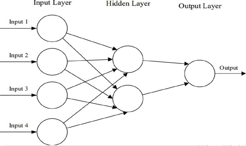
The basic structure of an ANN can be modeled as shown in Figure 1, which is comprised of an input layer, a hidden layer, and an output layer. This structure is the basis of several common ANN architectures, including but not limited to Feedforward Neural Networks (FNN), Restricted Boltzmann Machines (RBMs), and Recurrent Neural Networks (RNNs). As shown, we would load the input, usually in the form of a multidimensional vector to the input layer which will distribute it to the hidden layers. The hidden layers will then make decisions from the previous layer and weigh up how a stochastic change within itself detriments or improves the final output, and this is referred to as the process of learning. Having multiple hidden layers stacked upon each other is commonly called deep learning [59].
Figure 1 A simple three-layered feedforward neural network (FNN) [59].
3.2 Activation Functions
Neural networks can harness different activation functions to express complex features. Like the function of the neuron model of the human brain, the activation function here is a unit that determines which information should be transmitted to the next neuron. Each neuron in the neural network accepts the output value of the neurons from the previous layer as input and passes the processed value to the next layer. In a multilayer neural network, there is a function between two layers. This function is called the activation function, whose structure is shown in Figure 2.
Figure 2 General activation function structure [60].
In this figure, x represents the input feature; n features are input to the neuron j at the same time; w represents the weight value of the connection between the input feature xi and the neuron j; b represents the internal state of the neuron j, which is the bias value; and y is the output of the neuron j. is the activation function, which can be a Sigmoid function, tanh (x) function [61], Rectified Linear Unit [62], etc. The Sigmoid function is one of the most typical non-linear activation functions with an overall S-shape (Figure 3(a)). With the x value approaching 0, the gradient becomes steeper. The Sigmoid function can map a real number to (0, 1), so it can be used for binary classification problems. In addition, SENet [63] and MobileNet v3 [64] need to transform the output value to (0, 1) for the attention mechanism, which sigmoid is a good way to implement. Different from the Sigmoid, TANH function [61] (Figure 3(b)) can map a real number to (1, 1). Since the mean value of the output of TANH is 0, it can achieve a kind of normalization. This makes the next layer easier to learn. In addition, the Rectified Linear Unit (ReLU) [62] (Figure 3(c)) is another effective activation function. When x is less than 0, its function value is 0; when x is greater than or equal to 0, its function value is x itself. Compared to the Sigmoid function and TANH function, a significant advantage of using the ReLU function is that it can speed up learning. Sigmoid and TANH are involved in exponential operations that require division while computing derivatives, whereas the derivative of ReLU is a constant. Moreover, in the sigmoid and TANH function, if the value of x is too large or too small, the gradient of the function is pretty small, which can cause the function to converge slowly. However, when x is less than 0, the derivative of ReLU is 0, and when x is greater than 0, the derivative is 1, so it can obtain an ideal convergence effect. AlexNet [65], the best model in ILSVRC2012, uses ReLU as the activation function of the CNN-based model, which mitigates the gradient vanishing problem when the network is deep and verifies that the use of ReLU surpasses sigmoid in deep networks.
Figure 3 Diagrams of Sigmoid, Tanh, and ReLU functions.
3.3 Back-propagation Algorithm
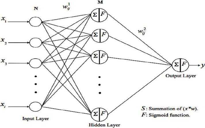
The back-propagation algorithm is one of the most widely used and popular techniques to optimize feedforward neural network training. It is highly suitable for problems in which no relationships are found between the output and input. Figure 4 illustrates the BP architecture in detail. It consists of an input layer, one or more hidden layers, and an output layer. Layers are connected sequentially starting from the input layer through the hidden layers to the output layer. Where the connections between layers contain weights and each layer includes one or more neurons.
Figure 4 Schematic representation of back-propagation architecture [70].
The basic idea behind BP is to minimize the overall output error gradually during the learning process. Whereas the training sets are estimated iteratively through the input layer to predict the correct output. The BP process is divided into two stages: forward and backward process. In the forward process, the BP architecture is described as: X are the inputs to the neural network with N neurons, are the weights of interconnections between inputs and hidden layers, and M neurons for the hidden layer. The hidden layer is defined by:
| (3) |
Where b is a bias input layer, the hidden layer will pass through activation function f (sigmoid function is used here):
| (4) |
After calculating the overall output by multiplying the output of the hidden layer neurons with the hidden layer weights , the final output will be:
| (5) |
The algorithm defines a loss function to measure the fit of the model. The small value of the loss function leads to better performance of the fitting procedure. The error function forward propagation can be defined as follows:
| (6) |
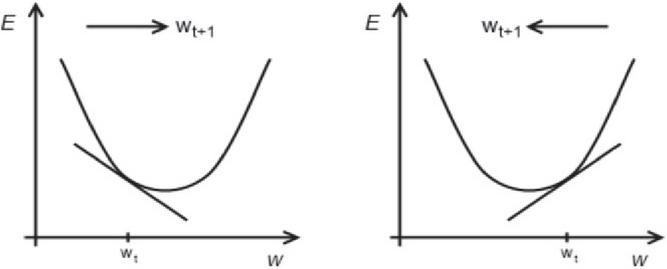
Where is the target value and is the number of data that is given to the network at each epoch of training. In the backward process, weights on the connections between all layers will be updated to minimize the error between the target (or desired) and output until finding the optimum weights with minimum E. For this purpose, a gradient descent algorithm is used. According to this algorithm, the gradient of the error function (dE/dW) is calculated concerning the weights to find a root. In particular, the weights are modified going in the opposite direction of the partial derivatives until a local minimum is reached. This idea is roughly illustrated in Figure 5 for a univariate error function. If the partial derivative is negative, the weight is increased (left part of the figure); if the partial derivative is positive, the weight is decreased (right part of the figure). After the weights are updated, the forward process is down again, this time with new weights. This cycle continues until the desired accuracy is reached.
Figure 5 Gradient descent algorithm illustrated for a univariate error function E(w).
3.4 Convolutional Neural Network (CNN)
A Convolutional neural network is a kind of feedforward neural network that can extract features from data with convolution structures. Different from the traditional feature extraction methods [66, 67], CNN does not need to extract features manually. The architecture of CNN is inspired by visual perception. A biological neuron corresponds to an artificial neuron; CNN kernels represent different receptors that can respond to various features; Compared with general artificial neural networks, CNN possesses many advantages, which are important reasons for its success in various image processing tasks: (1) Local connections. Each neuron is no longer connected to all neurons of the previous layer, but only to a small number of neurons, which is effective in reducing parameters and speeding up convergence; (2) Weight sharing. A group of connections can share the same weights, which reduces parameters further. (3) Down-sampling dimensionality reduction. A pooling layer harnesses the principle of image local correlation to down-sample an image, which can reduce the amount of data while retaining useful information. It can also reduce the number of parameters by removing trivial features. The three appealing characteristics make CNN one of the most representative algorithms in the deep learning field. To be specific, to build a CNN model, four components are typically needed. Convolution is a pivotal step for feature extraction. It involves sliding a window (often called a filter or kernel) across the input data. The outputs of convolution can be called feature maps. When setting a convolution kernel with a certain size, we will lose information in the border. Hence, padding is introduced to enlarge the input with zero value, which can adjust the size indirectly. Besides, for the sake of controlling the density of convolving, stride is employed. A larger stride will result in a lower density. After convolution, feature maps consist of a large number of features that are prone to causing overfitting problems [68]. As a result, pooling [69] (a.k.a. down-sampling) is proposed to obviate redundancy, including max pooling and average pooling. an average pooling layer performs down-sampling by dividing the input into rectangular pooling regions and computing the average values of each region, while in max pooling this is done by computing the maximum value. The procedure of a CNN is shown in Figure 6.
Figure 6 Procedure of a two-dimensional CNN.
4 A Surrogate Model Based on Deep Learning for Steady-state Heat Transfer Simulation
There are already several examples of research exploring the application of deep learning techniques within the physics and engineering communities [36–39], including applications for accelerating fluid simulations in graphics generation [40, 41] and shape optimization for drag reduction [42, 43]. These approaches have shown deep learning models perform exceptionally well in classification and regression tasks.
This work presents an equation-free approach based on deep learning algorithms for modeling physical phenomena, in which it presents a new method based on weakly supervised learning. Then this method is used to simulate heat transfer in a two-dimensional field. Firstly, in this section, the proposed method is introduced. Then the architecture and implementation of the proposed model will be described.
4.1 Approach
One of the goals of this research is to use deep learning algorithms to train a convolutional neural network to generate a model that can directly infer the solution of the Laplace Equation (1) when receiving the desired initial boundary conditions as input. One of the approaches of machine learning to solve problems is to use the supervised learning method its goal is learning a function (trained model) that maps data as feature vectors (input) to labels (output), based on example data-label pairs [44]. This method is shown in Figure 7. Supervised learning uses a loss function whose task is to compare the data generated from the network with the label corresponding to the input and calculate the amount of this difference as an error. The network is trained to reduce this error and to produce a supervised model. This method is completely data-driven, the accuracy of which is highly dependent on the amount of labeled data given to the network.
Figure 7 Model training by supervised method.
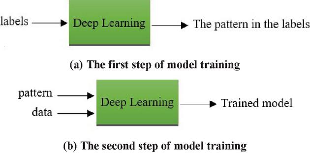
This research, by presenting a non-data-oriented approach, tries to make the training of the model possible with less labeled data and at the same time with high accuracy. The proposed approach to achieve this goal seeks a new and different definition for the loss function. For this purpose, in this method, the loss function focuses on the hidden pattern in the data instead of the data itself. The rules governing any phenomenon can be obtained directly through the data defining that phenomenon, and a loss function can be defined and produced from them, which calculates the degree of matching of the data generated from the network with the pattern that it infers and extracts from the data describing the phenomenon as a value, which shows the error of the data generated from the network. To generate this function, a learnable convolutional kernel has been used, which has a good potential to find patterns in the data and encrypt them in its parameters. When the pattern is extracted and encoded in the loss function, there is no need to use any data to train the model, and the network is trained unsupervised and without observing any labeled data during the learning process. Model training in this approach consists of two steps, As shown in Figure 8(a), in the first step, the existing pattern in the phenomenon is learned through a limited number of relevant labeled data. Then, in the second step, as shown in Figure 8(b), to generate the model, unsupervised training is performed using the pattern obtained from step 1 with unlabeled data (feature vectors). In Section 4.3, the details of the proposed method are fully described, including how to extract the pattern from thermal data and how to use it instead of labels (equilibrium conditions) for model training.
Figure 8 The steps of model training in the proposed method.
4.2 Network Architecture
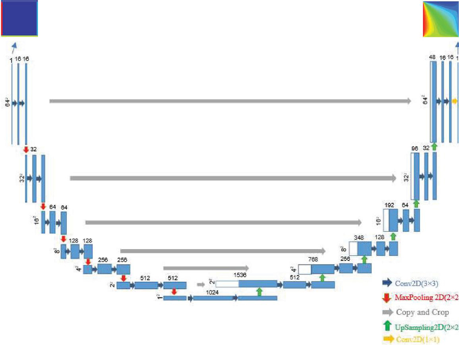
Convolutional neural networks (CNNs) are the most common architectures used in supervised deep learning techniques. CNNs are state-of-the-art architectures for classification, detection, and segmentation [37, 38] and surpass human performance in image classification [39]. CNNs are primarily used in the field of pattern recognition within images. This allows us to encode image-specific features into the architecture, making the network more suited for image-focused tasks whilst further reducing the parameters required to set up the model. The architecture of the network contains a two-dimensional convolutional encoder-decoder network adapted from the U-Net architecture [49]. The U-Net is based on a fully convolutional neural network. This architecture is used successfully in translating text and images [50–53]. The U-Net architecture of this network has two symmetrical paths (contracting and expanding), creating a U-shape. The contraction (downsampling) path is a traditional CNN for feature extraction that forms an encoder network. This network is comprised of several two-dimensional encoding convolutional layers that gradually decrease the input image size in each layer to reach an image of size in the bottleneck. The expanding path (upsampling) is used to preserve spatial information and forms a decoder network. The layers of this network inversely expand the reduced representation produced by the encoder to an input-sized image. Both paths are connected by skip connections to share a large amount of low-level information directly between the equivalent size layers in the two encoder and decoder networks using these connections to preserve the spatial features from the early layers [49]. The architecture is shown in Figure 9. Each blue box corresponds to a multi-channel feature map. The number of channels is denoted on top of the box. The x-y-size is provided at the lower left edge of the box. White boxes represent copied feature maps. The arrows denote the different operations.
Figure 9 Encoder-Decoder U-Net [49] architecture of the network (for 6464 pixels).
4.3 Implementation of the Proposed Method
In this section, the implementation steps of the proposed method to simulate steady-state heat transfer are described in detail.
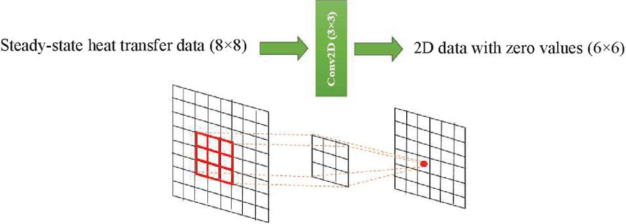
Figure 10 Network containing the steady-state temperature distribution pattern architecture.
4.3.1 The first step of implementation: Extraction of steady-state heat transfer pattern
In the first step, we tried to extract the pattern in the steady-state heat transfer directly from a limited number of thermal data (labels) in low dimensions () and small size (400) and encode it in a convolutional kernel. This data shows the temperature status (in degrees Celsius) of the points of a two-dimensional plate () in equilibrium conditions after applying heat to its 4 border edges. The convolutional kernel is supposed to learn the pattern in this data. In this step, a simple convolutional neural network was implemented according to Figure 10, which shows the architecture of this network. In this network, only a two-dimensional convolutional layer with a learnable kernel was used. In this layer, the number of features was set to 1, the activation was set to none, and the bias value was set to zero. To generate the data used for training the network, first, images with zero values and different random boundary conditions (temperatures of four edges) were generated and then it is given to a two-dimensional CFD simulator to calculate the steady-state temperature with high accuracy using the finite difference method. Then the obtained data with dimensions of was used as data (input) and two-dimensional data with dimensions of with zero values as labels (Output) for training the network. We seek to assign the 2D thermal field data to a specific category, like a 1-class classification problem. For this purpose, during the training of this network, we encode all the thermal data to a constant value so that the network directs them to this specific class. In this work, we set this class with a value of zero. During the training process of the network, the learnable convolution kernel passes over the thermal data and a data is produced in the output. This kernel is trying to set its weights in such a way that the average sum of the squares of the output nodes is minimized (close to zero). After several thousand iterations on randomly generated data points, this procedure learns the following kernel, shown in Figure 11.
Figure 11 The kernel resulting from the training of the network.
In the resulting kernel, all kernel nodes have a value close to zero except the central node and four adjacent nodes. The nodes have almost the same value, which is equal to a quarter of the value of the central node. The value obtained from the kernel passing through any point of the two-dimensional steady-state heat transfer data is almost zero. If is the temperature of node (i, j) in the conducting plane at the equilibrium moment, then by passing this kernel (Figure 11) through any point like node (i, j) of that conducting plate, Equation (2) appears. It means that the temperature at each point in the two-dimensional space with equilibrium conditions should be the average of its four adjacent points. This indicates the finite difference method described in Section 2. It is by iteration of this rule that the finite-difference method for solving partial differential equations typically solves this problem with high accuracy. This shows that it is possible to learn the local laws that define the equilibrium conditions directly from these data without needing to prepare thermal data in high volumes and dimensions.
4.3.2 The Second step of implementation: generating the steady-state temperature distribution predictor model
In the previous step, we obtained the pattern of the class related to the thermal data, which defines the two-dimensional temperature distribution. By extracting the pattern in the limited labeled data in the previous step, there is no need to prepare labels (equilibrium conditions) for model training. The correct output is the data that is closer to the pattern (which represents the correct equilibrium conditions). We intend to direct the data generated from the network to a specific class that belongs to thermal equilibrium, and we do this by imposing constraints on the output of the network through the error defined in Equation (7). For this purpose, the output data from the network should be checked immediately by the network containing this pattern (Figure 10) and its error calculated. The more accurately the output data from the network satisfies the equilibrium conditions defined in the kernel, the closer the error calculated by this layer will be to zero. Therefore, the training of this network is done in an unsupervised way without observing the labels (steady-state data) only by applying restrictions on the data output from the network by the kernel containing the pattern.
| (7) |
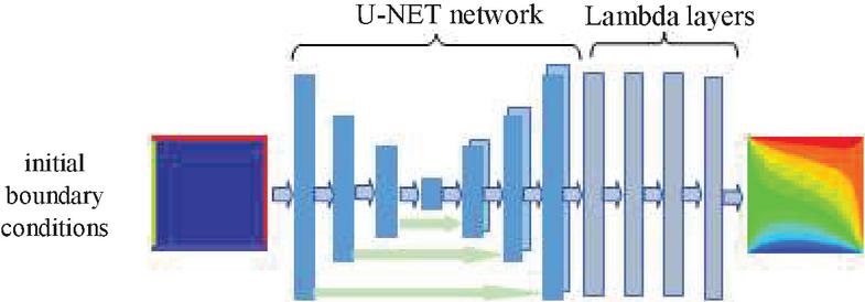
The architecture of this network uses a U-Net architecture, the details of which are shown in Figure 9. To transfer the values of the temperature boundary conditions of the input data to the output data boundaries of the network, four lambda layers (to transfer the temperatures of the four edges) have been used to the end of the U-Net network so that the network produces the steady-state temperatures according to the temperature boundary conditions of the input data. The resulting network architecture is shown in Figure 12. In this network, we used ReLU function in each convolutional layer due to its better overall performance and higher convergence speed than other activation functions. How this function works is explained in Section 3.2. To train this network in an unsupervised way, according to Figure 13, the network containing the steady-state distribution temperature pattern (Figure 10) is connected to the end of the network (Figure 12) while its kernel is frozen to calculate the errors of the output data produced from it according to Equation (7). The input is a square plate with zero values. The four sides of the plate are set with four random temperatures between 0 and 100 degrees Celsius.
Figure 12 The steady-state temperature distribution predictor network architecture.
Figure 13 The steady-state temperature distribution predictor network training.
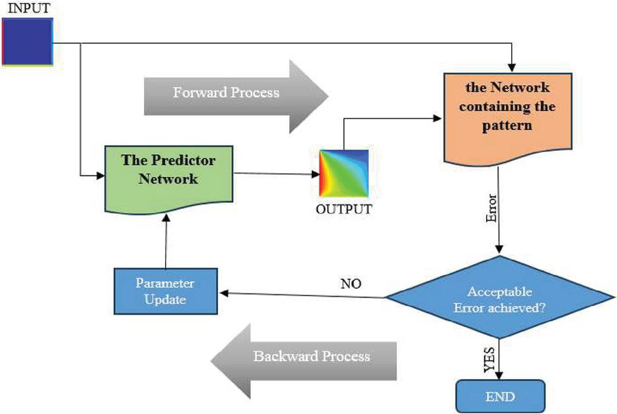
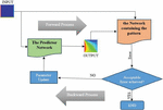
Figure 14 Flowchart of the predictor network training using the back-propagation algorithm.
This network uses the back-propagation algorithm to adjust its weights and parameters, the way the algorithm works is explained in Section 3.3. Figure 14 shows the flowchart of predictor network training using this algorithm. First, square plates with zero temperature and with different temperature boundary conditions enter the network. Then, in the forward process, by passing the data through different hidden layers of the network, calculation operations are performed on the data and the initial weights of the layers. In this operation, the output data values from the input layer and hidden layers are obtained according to Equations (3) and (5), respectively. The function used in each layer is ReLU. Then the output generated from the network and its related boundary conditions are given to the Network containing the pattern (whose parameters are frozen) to calculate the error rate and its deviation from the equilibrium temperature pattern using Equation (7). In the next step, this error is checked and if the model has not reached the acceptable accuracy, the backward process is started to update the weights to obtain a lower error. In this step, the network parameters are optimized using the gradient descent algorithm (explained in Section 3.3). This cycle stops when the network achieves the desired accuracy.
5 Analyzing and Evaluating the Results of the Proposed and the Supervised Models
In this section, in addition to the proposed model, a supervised model has been designed and trained using the labeled steady-state heat transfer data to evaluate the efficiency of the proposed model in equilibrium condition simulation. The network architecture used in the proposed model comprised 12 hidden layers. It includes 6 encoder layers and 6 decoder layers in the first part, and 4 lambda layers in the second part to transfer four boundary values of the input to the output.
The architecture of the supervised model is the same as the U-Net network in the proposed model. The architecture of both models is considered in the same conditions in terms of the number of main layers, the number of learnable parameters as well as the number of training data used for training. The input data to the supervised model network is 5000 matrices with dimensions of with zero values. The four edges are set with four different numbers between 0 and 100. The labels are the equilibrium conditions corresponding to the square input data. In this experiment, the data generated by the finite difference method obtained using the CFD simulation is used as an accuracy criterion to measure the accuracy of the outputs generated by the networks of both models. In the model created by the proposed method, only 400 data with dimensions of were used to extract the steady-state heat transfer pattern during this experiment. In this model, the network is trained to minimize the error defined in Equation (7) in an unsupervised way without directly observing any heat distribution data. In contrast, the supervised model used 5,000 steady-state heat transfer labeled data to train its network. The two models have been compared and evaluated with each other from different aspects such as generated output data, changes in the percentage of average absolute error during the training process, as well as the method and process of learning to produce the steady state heat transfer data.
5.1 Comparison and Evaluation of Outputs Produced by Proposed and Supervised Models
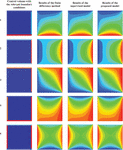
Figure 15 shows the outputs simulated by the proposed model and the supervised model. The first column of the figure shows the input data in this
Figure 15 Results of the equilibrium heat distribution simulation with different boundary conditions in size of 64 64 64, using finite difference method, supervised and proposed models.
experiment. The input data to the models are matrices of size with zero values, the 4 edges of which are set with 4 different temperatures between 0 and 100 degrees Celsius. Each matrix shows the thermal conditions of the conductive plate at the first moment of heat application. Therefore, the only non-zero entries in the input are at the boundaries. These areas are marked with dark blue in the figure. The 4 edges around the plate, which are marked with different colors, represent the different temperatures applied to the conductive plate in the first moment. The boundary conditions for the ten input data displayed in this column are listed in 4 different temperatures in Table 1. The data displayed in the next three columns show the temperature distribution of the input data at any point on the screen using the three different methods after the heat transfer process converges to an equilibrium temperature distribution. The data solved by the finite difference method are assumed as real equilibrium conditions and placed in the second column. The next two columns show the outputs obtained from the two proposed and supervised models in the relevant boundary conditions, respectively.
By comparing the outputs of the two models with the corresponding outputs in the finite difference method, it is obtained that the network in the proposed model, despite not observing the labeling data during network training, has produced a more accurate steady-state temperature distribution simulation compared to the supervised model. Of course, the results obtained from both models are somewhat similar to the data produced by the finite difference method.
Table 1 Boundary conditions of the input data shown in Figure 15
| Number | Left | Right | Bottom | Top |
| 1 | 9 | 23 | 71 | 0 |
| 2 | 45 | 94 | 55 | 55 |
| 3 | 5 | 45 | 2 | 40 |
| 4 | 84 | 99 | 92 | 3 |
| 5 | 74 | 71 | 12 | 29 |
| 6 | 34 | 55 | 9 | 60 |
| 7 | 38 | 0 | 12 | 59 |
| 8 | 11 | 78 | 5 | 12 |
| 9 | 100 | 21 | 68.44 | 6.9 |
| 10 | 34 | 11 | 12 | 29 |
5.2 Comparison of Cost of Computations and data Consumption for Fully Training of Proposed and Supervised Model
Table 2 shows the two models in terms of the number of data used, the dimensions of each data, the time taken to fully train the models, and the data errors produced by the two models with MAPE (Mean absolute percentage error) and MSE (Mean squared error) values. According to these results, the proposed model (kernel-based model) with its different approach to defining the loss function, has reduced the amount of data consumption to less than one-twelfth compared to the supervised method (400 versus 5000 data). In addition, the dimensions of each data used in this method are 64 times smaller than the data used in the supervised method ( versus ), and despite all this, this model is more accurate with fewer simulation errors (MAPE and MSE) compared to the supervised model. The MAPE value for the supervised model is 1.53%, while this value for the kernel-based model is equal to 0.68% despite using less than one-tenth of the data. Also, the value of MSE in the supervised model is about three times higher than in the kernel-based model. 0.78 vs. 0.23.
Table 2 Comparison of proposed and supervised models from different aspects
| Model | Data | Data | Training | ||
| Type | Dimensions (Pixel) | Size (Number) | Time (Hour) | MAPE | MSE |
| Supervised model | 6464 | 5000 | 20 | %1.53 | 0.78 |
| Proposed model | 88 | 400 | 11 | %0.68 | 0.23 |
5.3 Comparison of Changes in the Output Error (MAPE) of Proposed and Supervised Models During the Training Step
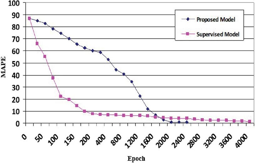
Figure 16 shows the changes in the percentage of average per-pixel output error (MAPE) of proposed and supervised models during different periods of the training process in this experiment. The pink curve corresponds to the supervised model, and the blue curve corresponds to the proposed model. In this figure, the horizontal and vertical axes represent the training epoch and the average per-pixel output error corresponding to the relevant training epoch, respectively. The accuracy of the two models has been measured using the MAPE formula [54] as follows.
| (8) |
y is the correct equilibrium temperature distribution matrix obtained using the finite difference method in this experiment. y also represents the temperature distribution matrix predicted by the relevant method. The mean operator calculates the average values of the resulting matrix.
Figure 16 Comparing the mean absolute percentage error (MAPE) curves of the two proposed and supervised models during the training process.
As for the training procedure, experience so far indicates that while training deep neural networks, it is often useful to reduce the learning rate as the training progresses [55]. In this experiment, using the Adam optimizer [56], the learning rates of the two models were set with different values in descending order from 10 to 10 during consecutive courses during the training process as shown in Table 3. The training of the supervised and proposed models has been done during 4000 and 2200 epochs, respectively, with a batch size of 128 samples. Every epoch of the optimizer on a single NVIDIA Tesla K80 GPU card takes around 18 seconds, for both models. Before starting the learning process, the weights of the networks of both models were randomly set with identical values. Therefore, both have started the training process with the same weights. At the beginning of the learning process, the mean absolute percentage error (MAPE) for both models is 87%. According to Figure 16, the error reduction process is performed at a very high speed in early training when the simulation error of both networks is high. However, this process gradually becomes slower by gaining more accuracy. In the initial moments of training, the simulation error curve of the supervised model has a much steeper slope than the proposed model, which shows that in early training the learning ability of the supervised model is much higher than the proposed model. In this model, the error reduction process does not last long, so it slows down sharply from the 200th epoch onwards. Finally, the training of this model stops after about 4000 epochs, gaining an average error of 1.53% per pixel. In contrast, it has lasted longer in the supervised model, although the error reduction process is relatively slow from the beginning. In this model, the error reduction process has become faster gradually with more training epochs. Until the curves of both models intersected each other at the epoch 1800 with an error rate of 4.9%. From this epoch onwards, the proposed model has fewer errors than the supervised model. The slope of the curve related to the mentioned model slows down after about 2000 epochs, and finally, this model succeeds in obtaining a lower error rate with a smaller number of training epochs. The training of this model ends after 2400 training epochs with an average output error rate of 0.68% per pixel. From the analysis and comparison of the two curves, it can be inferred that the learning speed of the supervised model is much higher in the early training, but then the proposed model succeeds in gaining higher accuracy with a smaller number of training epochs. This indicates the high learning capability of the proposed model in simulating the two-dimensional heat transformation. Moreover, the training epochs of the proposed model are faster than the supervised model with 1600 fewer epochs.
Table 3 The learning rates of the two proposed and supervised models during different training epochs
| Supervised Model | Proposed Model | ||
| Learning Rate | Epoch | Learning Rate | Epoch |
| 10 | 300 | 10 | 600 |
| 8 10 | 2100 | 8 10 | 1000 |
| 2 10 | 1000 | 5 10 | 200 |
| 10 | 200 | 10 | 200 |
| 10 | 200 | 5 10 | 200 |
| 10 | 200 | 10 | 200 |
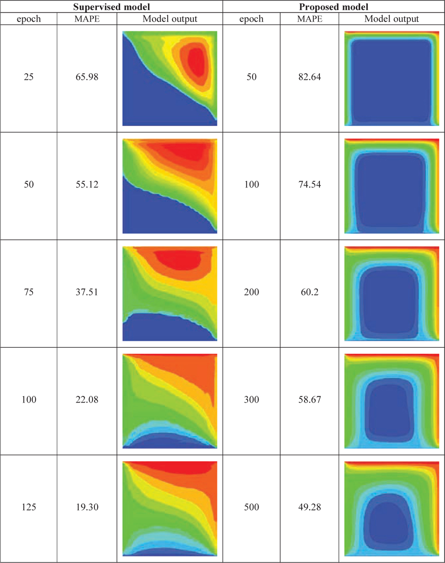
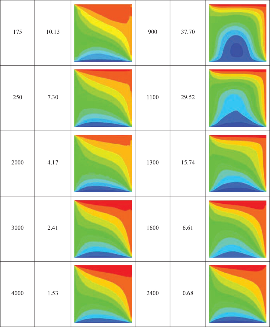
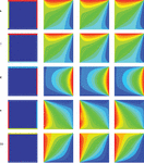
Table 4 Comparison of the learning process of the two proposed and supervised models during the training process
5.4 Comparing the Learning Process of the Proposed and Supervised Models During the Training Process
Table 4 shows the learning process of the two proposed and supervised models in steady-state heat transfer simulation during different training epochs and compares them with each other. The initial temperature distribution of the square control volume shown in the table at the left, right, bottom, and top borders of the conductive plate is 34, 55, 9, and 60C, respectively. The information displayed in each column of the table shows the output of the desired model and the average per-pixel output error of the model in the relevant training epoch. Although the two models eventually produced the same output, they each adopted a different learning method to produce the desired output. According to the information in the left-hand column of the table, which describes the learning process of the supervised model, early in the training, the network tends to generate outputs that draw an overall structure of the equilibrium condition on the output by observing the steady-state heat transformation data. It then slowly adds more detail to the desired output. In this model, the fundamental changes are applied in the first training epochs and intangible changes are made to the output image from the 250 epoch onwards. The right-hand column of the table shows the output of the proposed model in each training epoch. The proposed model tends to reduce the value obtained by passing the kernel containing the equilibrium conditions pattern across the output. Therefore, it is trained by this criterion that the temperature of each point should be the average of the temperatures of the four adjacent points. Consequently, a plate with constant temperatures also satisfies the desired conditions. Since the borders of a plate with dimensions of form a relatively small fraction of the whole plate, early in the training, the model tries to satisfy the pattern in the kernel by producing outputs in which the entire plate is zero except for its four borders. As the learning process progresses and to further reduce the amount obtained from the kernel passing across the output, the network gradually moves towards producing outputs that follow this pattern to a greater extent. Therefore, in the early training, compared to the proposed model, there is a large distance between the correct output (correct equilibrium heat distribution), and the learning process is very slow. However, the output produced by this model is more accurate. This is because it follows the principle of the equilibrium temperature pattern encrypted in the kernel. The supervised model draws an overall structure of the equilibrium heat distribution from the beginning and then completes it by adding more details of the equilibrium temperature conditions. However, in the proposed model, a completely opposite procedure occurs. In this model, the temperature lines are smooth from the beginning and possess details, but the desired overall structure is achieved by more training epochs. Therefore, the model has a high error rate early in the learning process, but over time and with the formation of the overall structure of the equilibrium heat distribution, the error reduction process proceeds faster than the supervised model.
6 Comparison and Evaluation of the Present Work for the 2D Heat Transfer
In this section, we examined the models presented in the previous sections that have performed two-dimensional steady-state heat transfer simulation after applying specified temperatures to the edges of a conductive plate using huge data. The number of data used in the first and second research is more than 10 times and 100 times the data used in the proposed model of this article, respectively. Both models have used data-driven methods to train a U-Net neural network. We compared the two models in terms of simulation accuracy, the number of data used, and the dimensions of each image data with the proposed model. The details of these results have been examined and analyzed in the next two subsections.
6.1 Model Based on Generative Adversarial Network (cGAN)
Research [57] presented a new data-driven model based on a Generative Adversarial Network, which, like the current research, performs two-dimensional steady-state heat transfer on a conductive plate in different temperature boundary conditions [57]. A U-Net network is used in the architecture of this work as in the present work.
The results of comparing these models from different aspects (including the number of data used, the dimensions of each data, and simulation accuracy) are shown in Table 5. In this table, the cGAN-based model introduced in the mentioned research [57] is named model A. According to these results, the number of data used and the size of each data in the cGAN-based model are about 9 and 64 times more than our proposed model (kernel-based model), respectively. And yet, our model has achieved higher accuracy despite using much less data. The value of MAPE for our model is %0.68, which is about %0.32 less than the cGAN-based model.
6.2 Model Based on an Advanced Deep Neural Network
Research [58] has employed an advanced type of artificial intelligence, a deep neural network, to learn the physics of conduction heat transfer in two-dimensional geometries using a large dataset of observations [58]. A dataset containing 44,160 samples is produced using the conventional finite difference method on a uniform grid of . The dataset includes four geometries of the square, triangular, regular hexagonal, and regular octagonal with random sizes and random Dirichlet boundary conditions. Then, the dataset of the solved problems was introduced to a convolutional Deep Neural Network (DNN) to learn the physics of 2D heat transfer without knowing the partial differential equation underlying the conduction heat transfer.
The results of comparing the model with the proposed model from different aspects are shown in Table 5. In this table, the model that is introduced in the mentioned research [58] is named model B. According to the results in the Table, the number of data used and the dimensions of each data in this model are about 110 and 64 times more than our proposed model (kernel-based model), respectively. That is, the number of data used has increased to more than 9 times more than the cGAN-based model, and thus the value of MSE has been reduced for it compared to our proposed model (0.0055 versus 0.23). Therefore, our proposed model is a good option for problems where we have access to very limited data in dimension and size to solve, while we need an acceptable level of accuracy.
Table 5 Comparison results of proposed and presented models [57,50] from different aspects
| Model Type | Data Dimensions | Data Size | MAPE | MSE |
| Model A [57] | 4850 | %1 | – | |
| Model B [58] | 44160 | – | 0.0055 | |
| Proposed Model | 400 | %0.68 | 0.23 |
7 Conclusion
In this study, the two-dimensional steady-state heat conduction problem is investigated. For this purpose, an equation-free approach is presented that uses deep learning algorithms instead of governing differential equations to simulate the physics of conduction heat transfer. The proposed model can simulate the equilibrium heat distribution without using governing equations under arbitrary boundary conditions outside the range of training data observed by the network and with only a small amount of thermal data, with acceptable accuracy. To train the model, a small data set, containing 400 data from square plates with dimensions of with different boundary conditions, was prepared. The actual temperature distribution in each of the plates along with the boundary conditions was generated using the finite difference method. This data was used to extract the steady-state temperature pattern and encode it in a convolutional kernel. Then, this kernel was used as a loss function to calculate the network error in the steady-state temperature distribution simulation so that the network does not need thermal data in high dimensions () as labels. For this, a network with U-Net architecture was used and it was trained using a kernel containing a pattern. The produced model was compared with other models in different aspects. The results showed that the presented model based on a kernel, despite using only 400 data in low dimensions has managed to obtain a lower value of MAPE and MSE in simulating the actual steady-state temperature distribution than the supervised model that used a large set of 5000 data in high dimensions () (0.68% vs. 1.53% in MAPE value and 0.23 vs. 0.78 in MSE value). The results also showed that with a different definition of the loss function in model training, the learning process will be different subsequently, even if the output results of the two models are the same. According to Table 4, which shows the learning process of two models during different periods, the supervised model tries to create a general structure of equilibrium conditions in the output at the beginning of the learning process. While the kernel-based model tries to produce a temperature distribution that covers a large part of the screen with zero temperature values. The learning process of the two models in Figure 16 shows that the supervised model has a higher learning speed at the beginning of the learning process than the kernel-based model, but gradually as it approaches higher accuracies, the learning speed drops drastically. This procedure happens in the opposite way in the kernel-based model.
In the end, the kernel-based model was compared with two models introduced in two other studies, which, like the present work, have performed the simulation of two-dimensional steady-state heat transfer in different boundary conditions. The comparison results showed that the kernel-based model, despite using one-tenth of the thermal data used in the cGAN-based model (400 vs 4850 data) and with lower dimensions ( vs ), was able to compute temperature distribution with less error (0.68% vs 1%). However, the model presented in [58] has succeeded in obtaining higher accuracy by increasing the data to more than a hundred times higher dimensions.
This work points to the possibility of extracting existing laws and patterns in physical phenomena and encoding them in neural networks that no longer need to find the governing differential equations or prepare huge data related to the phenomenon. In principle, the equation-free method presented in this article is a suitable solution for solving those problems that seek to simulate a physical phenomenon with acceptable accuracy despite the small amount of data.
References
[1] Mattheij, R., Sjoerd, W., “Partial differential equations: modeling, analysis, computation”, Society for Industrial and Applied Mathematics, (2005).
[2] Sadeghi, E, S., Cronin, L.,Sadeghi, S., Pakzad, S., “Input estimation of nonlinear systems using probabilistic neural network”, Journal of Mechanical Systems and Signal Processing, Vol. 166, No. 9, (2021).
[3] Moghanlo, S., Alavinejad, M., Oskoei, V., Najafi, H., “Using artificial neural networks to model the impacts of climate change on dust phenomenon in the Zanjan region”, Journal of Urban Climate, Vol. 35, (2021).
[4] Graf, R.; Kolerski, T.; Zhu, S., “Predicting Ice Phenomena in a River Using the Artificial Neural Network and Extreme Gradient Boosting”, Resources, Vol. 11, No. 2, (2022).
[5] Pichi, F., Ballarin, F., Rozza, G., “An artificial neural network approach to bifurcating phenomena in computational fluid dynamics”, Journal of Computers & Fluids, Vol. 254, (2023).
[6] Ma, J., Wang, J., Han, Y., Dong, S., “Towards data-driven modeling for complex contact phenomena via self-optimized artificial neural network methodology”, Journal of Mechanism and Machine Theory, Vol. 182, (2023).
[7] Bongard, J., Lipson, H., “Automated reverse engineering of nonlinear dynamical systems”, National Acad Sciences, USA 104, (2007), 9943–9948.
[8] Schmidt, M., Lipson, H., “Distilling free-form natural laws from experimental data”, Journal of Science, (2009), 81–85.
[9] Lusch, B., Kutz, J.N., Brunton, S.L., “Deep learning for universal linear embeddings of nonlinear dynamics”, Journal of Nature Communications, (2018).
[10] Ruthotto, L., Osher, S., Li, W., Nurbekyan, L., “A machine learning framework for solving high-dimensional mean field game and mean field control problems”, Journal of PNAS, Vol. 117, No. 17, (2020), 9183–9193.
[11] Ding, Y., Hua, L., Li, S., “Research on computer vision enhancement in intelligent robot based on machine learning and deep learning”, Journal of Neural Computing and Applications, Vol. 34, (2022), 2623–2635.
[12] Lauriola, I., Lavelli, A., Aiolli, F., “An introduction to deep learning in natural language processing: Models, techniques, and tools”, Journal of Neurocomputing, Vol. 470, (2022), 443–456.
[13] Johnson, M., Schuster, M., Le, Q., Krikun, M., Wu, Y., Chen, Z., Thorat, N., Viégas, F., Wattenberg, M., Corrado, G., Hughes, M., & Dean, J., “Google’s Multilingual Neural Machine Translation System: Enabling Zero-Shot Translation”, Transactions of the Association for Computational Linguistics, Vol. 5, (2017), 339–351.
[14] Gumbs, A., Grasso, V., Bourdel, N., Croner, R., Spolverato, G., Frigerio, I., Illanes, A., Abu Hilal, A., Park, A., Elyan, E., “The Advances in Computer Vision That Are Enabling More Autonomous Actions in Surgery: A Systematic Review of the Literature”, Vol. 22, No. 13, (2022).
[15] Thepade, S. D., Dindorkar, M.R., Chaudhari, P.R., Bang, S.V., “Enhanced Face Presentation Attack Prevention Employing Feature Fusion of Pre-trained Deep Convolutional Neural Network Model and Thepade’s Sorted Block Truncation Coding”, International Journal of Engineering (IJE), Transactions A: Basics, Vol. 36, No. 04, (2023), 807–816.
[16] El-Amir, H., Hamdy, M., “Deep Learning Pipeline: Building a Deep Learning Model with TensorFlow”, Apress, (2019).
[17] Venigandla, K., Tatikonda, V., “Improving Diagnostic Imaging Analysis with RPA and Deep Learning Technologies ”, Journal of Power System Technology, Vol. 45, No. 4, (2021).
[18] Liu, X., Gao, K., Liu, B., Pan, C., “Advances in Deep Learning-Based Medical Image Analysis”, Journal of Health Data Science, (2021).
[19] Ramcharan, A., Baranowski, K., McCloskey, P., Ahmed, B., “Deep Learning for Image-Based Cassava Disease Detection”, Journal of Frontiers in Plant Science, Vol. 8, (2017).
[20] Issa, D., Demirci, M.F., Yazici,A., “Speech emotion recognition with deep convolutional neural networks”, Journal of Biomedical Signal Processing and Control, Volume 59, (2020).
[21] Saleem, N., Khattak, M., Qazi, A., “Supervised Speech Enhancement Based on Deep Neural Network”, Journal of Intelligent & Fuzzy Systems, Vol. 37, No. 4, (2019), 5187–5201.
[22] Wang, D., Chen, J., “Supervised Speech Separation Based on Deep Learning: An Overview”, in IEEE/ACM Transactions on Audio, Speech, and Language Processing, Vol. 26, No. 10, (2018), 1702–1726.
[23] Chan, Z., Lau, C., Thang, K., “Visual Speech Recognition of Lips Images Using Convolutional Neural Network in VGG-M Model”, Journal of Information Hiding and Multimedia Signal Processing, Vol. 11, No. 3, (2020).
[24] Song, Z., “English speech recognition based on deep learning with multiple features”, Journal of Computing, Vol. 102, (2020), 663–682.
[25] Araújo, A., Pereira, A., Benevenuto, F., “A comparative study of machine translation for multilingual sentence-level sentiment analysis”, Journal of Information Sciences, Vol. 512, (2020).
[26] Andrabi, A., Wahid, A., “Machine Translation System Using Deep Learning for English to Urdu”, Journal of Computational Intelligence and Neuroscience, (2022).
[27] Petousis, P., Han, S., Aberle, D., Bui, A., “Prediction of lung cancer incidence on the low-dose computed tomography arm of the National Lung Screening Trial: A dynamic Bayesian network”, Journal of Artificial Intelligence in Medicine, Vol. 72, (2016), 42–55.
[28] Aberle, D., Adams, A., Berg, C., Black, W., “Reduced lung-cancer mortality with low-dose computed tomographic screening”, Journal of National Lung Screening Trial Research Team, (2011).
[29] D’Souza, G., Siddalingaswamy, P.C., Pandya, M.A., “AlterNet-K: a small and compact model for the detection of glaucoma”, Journal of Biomedical Engineering Letter, Vol. 14, (2024), 23–33.
[30] Zhou, Z., “A brief introduction to weakly supervised learning”, Journal of National Science Review, Vol. 5, No. 1, (2018), 44–53.
[31] Wang, R., Chen, B., Meng, D., Wang, L., “Weakly Supervised Lesion Detection from Fundus Images”, in IEEE Transactions on Medical Imaging, Vol. 38, No. 6, (2019), 1501–1512.
[32] Nguyen-Duc, T., Yoo, I., Thomas, L., Kuan, A., “Weakly supervised learning in deformable EM image registration using slice interpolation”, In IEEE 16th International Symposium on Biomedical Imaging, (2019), 670–673.
[33] Costa, P., Galdran, A., Smailagic, A., Campilho, A., “A weakly-supervised framework for interpretable diabetic retinopathy detection on retinal images”, IEEE Access 6, (2018), 18747–18758.
[34] Ganji, D., Sabzehmeidani, Y., Sedighiamiri, A., “Nonlinear System in Heat Transfer Mathematical Modeling and Analytical Methods”, (2018), 35–36.
[35] Daileda, R. C., “The two-dimensional heat equation”, Trinity University, San Antonio, Texas, (2012).
[36] Lu, C., Liu, Q., Sun, Q., Hsieh, C., Zhang, S., Shi, L., Lee, C., “Deep Learning for Optoelectronic Properties of Organic Semiconductors”, Journal of Physical Chemistry, Vol. 124, No. 13, (2020), 7048–7060.
[37] Ryczko, K., Strubbe, D., Tamblyn, I., “Deep Learning and Density Functional Theory”, (2019).
[38] Bikmukhametov, T., Jäschke, J., “Combining machine learning and process engineering physics towards enhanced accuracy and explainability of data-driven models”, Elsevier, Vol. 138, (2020).
[39] Frank, M., Drikakis, D., Charissis, V., “Machine-Learning Methods for Computational Science and Engineering”, Computation, (2020).
[40] Kochkov, D., Smith, J. A., Alieva, A., Hoyer, S., “Machine learning–accelerated computational fluid dynamics”, Journal of PNAS, University of California, Vol. 118, No. 21, (2021).
[41] Mario, l., Stathi, F., Anil A. B., Chris D. C., “Current and emerging deep-learning methods for the simulation of fluid dynam”, Journal of Proc. R. Soc. A, Vol. 479, No. 2275, (2023).
[42] Li, J., Zhang, M., Martins, J., Shu, C., “Efficient Aerodynamic Shape Optimization with Deep-Learning-Based Geometric Filtering”, AIAA Journal, Vol. 58, No. 10, (2020).
[43] Yan, X., Zhu, J., Kuang, M., Wang, X., “Aerodynamic shape optimization using a novel optimizer based on machine learning techniques”, Journal of Aerospace Science and Technology, Vol. 86, (2019).
[44] J.Russell, S., Norvig, P., “Artificial Intelligence: A Modern Approach, Third Edition”, Prentice Hall, (2010).
[45] Talo, M., “Automated classification of histopathology images using transfer learning”, Journal of Artificial Intelligence in Medicine, Vol. 101, (2019).
[46] Yousefi, S., Nie, Y., “Transfer Learning from Nucleus Detection to Classification in Histopathology Images”, IEEE 16th International Symposium on Biomedical Imaging, Venice, Italy, (2019).
[47] Ker, J., Wang, L., Rao, J., Lim, T., “Deep Learning Applications in Medical Image Analysis”, in IEEE Access, Vol. 6, (2018), 9375–9389.
[48] Aljuaid, A., Anwar, M., “Survey of Supervised Learning for Medical Image Processing”, Journal of Computer Science, (2022).
[49] Ronneberger, O., Fischer, P., Brox, T., “U-Net: Convolutional Networks for Biomedical Image Segmentation”, in International Conference on Medical Image Computing and Computer-Assisted Intervention, Springer International Publishing, (2015), 234–241.
[50] Jiang, J., Hu, Y. C., Tyagi, N., Zhang, P., Rimner, A., Mageras, G. S., Deasy, J. O., Veeraraghavan, H., “Tumor-aware, Adversarial Domain Adaptation from CT to MRI for Lung Cancer Segmentation”, Medical image computing and computer-assisted intervention, (2018), 777–785.
[51] Hinton, G. E., Salakhutdinov, R. R., “Reducing the dimensionality of data with neural networks”, Journal of Science, New York, N.Y., Vol. 313, No. 5786, (2006), 504.
[52] Yin, XX., Sun, L., Fu, Y., Lu, R., Zhang, Y., “U-Net-Based Medical Image Segmentation”, Journal of Healthc Eng, (2022).
[53] Siddique, N., Paheding, S., Elkin, C., Devabhaktuni, V., “U-Net and Its Variants for Medical Image Segmentation: A Review of Theory and Applications”, in IEEE Access, Vol. 9, (2021).
[54] Chicco, D., Warrens, M. J., Jurman, G., “ The coefficient of determination R-squaredis more informative than SMAPE, MAE, MAPE, MSE and RMSE in regression analysis evaluation”, Journal of Computer Science, (2021).
[55] Raissi, M., Yazdani, A., Karniadakis, G., “Hidden Fluid Mechanics: A Navier-Stokes Informed Deep Learning Framework for Assimilating Flow Visualization Data”, Journal of Science, (2018).
[56] Kingma, D. P., Ba, j., “Adam: A Method for Stochastic Optimization”, computer science, conference paper at the 3rd International Conference for Learning Representations, San Diego, (2014).
[57] Barati, A., Gomes, J., Pande, V., “Deep Learning the Physics of Transport Phenomena”, (2017).
[58] Edalatifar, M., Tavakoli, M. B., Ghalambaz, M., Setoudeh, F., “Using deep learning to learn physics of conduction heat transfer”, Journal of Thermal Analysis and Calorimetry, (2020).
[59] O’Shea, K., Nash, R., “An Introduction to Convolutional Neural Network”, Journal of Neural and Evolutionary Computing, (2015).
[60] Li, z., Yang, w., Peng, S., Liu, S., “A Survey of Convolutional Neural Networks: Analysis”, IEEE Transactions on Neural Networks and Learning Systems, Vol. 33, No. 12, (2022).
[61] B. L. Lecun, Y., Bengio, Y., et al., “Gradient-based learning applied to document recognition,” Proceedings of the IEEE, Vol. 86, No. 11, (1998), 2278–2324.
[62] Nair, v., Hinton, G. E., “Rectified Linear Units Improve Restricted Boltzmann Machines Vinod Nair”, (2010).
[63] Hu, J., Shen, L., Albanie, S., Sun, G., Wu, E., “Squeeze-and Excitation Networks.”, Journal of Computer Science, (2019).
[64] Howard, A., Chu, G., Chen, L., Chen, B., Tan, M., Wang, W., Zhu, Y., “Searching for MobileNetV3,” (2019).
[65] Krizhevsky, A., Sutskever, I., Hinton, G., “ImageNet Classification with Deep Convolutional Neural Networks,” Journal of Advances in Neural Information Processing Systems, vol. 25, no. 2, (2012).
[66] Cruz-Mota, J., Bogdanova, I., Paquier, B., Bierlaire, M., “Scale Invariant Feature Transform on the Sphere: Theory and Applications”, Journal of Computer Vision, (2012), 217–241.
[67] Ahonen, T., Hadid, A., Pietikäinen, M., “Face description with local binary patterns: application to face recognition”, Journal of IEEE Trans Pattern Anal Mach Intell, (2006).
[68] Hawkins, D. M., “The problem of overfitting”, Journal of Chemical Information and computer sciences, Vol. 44, No. 1, (2004).
[69] Gholamalinezhad, G., Khosravi, H., “Pooling Methods in Deep Neural Networks, a Review”, Journal of Computer Science, (2020).
[70] Hameed, A., Karlik, B., Shukri, M., “Back-propagation Algorithm with Variable Adaptive Momentum”, Journal of LATEX Templates, (2016).
Biographies

Somaye Afzali received her M.Sc. in Information Technology Engineering from University of Qom in 2020. Her research interests include AI and Machine Learning Applications in Computational Science and Engineering.

Mohammad Kazem Moayyedi received his Ph.D. in Aerospace Engineering from Sharif University of Technology in 2009. He is currently Associate Professor of Mechanical Engineering, the Director of CFD Turbulence and Combustion Research Lab. and the Director of Institute of Aerospace Studies at the University of Qom (Iran). His research interests include CFD, Geophysical Fluid Mechanics, Turbulence, and Machine Learning Applications in Mechanical Science and Engineering.

Faranak Fotouhi-Ghazvini received her MEng degree in Telecommunication Engineering from King’s College London (UK) in 2001 (1st class), and her Ph.D. degree from Bradford University (UK), Department of Informatics in 2011. She is an Assistant Professor at the Department of Computer Engineering and Information Technology and the Director of IoT and Smart Environments Research Lab. in University of Qom. Her research interests include Pervasive Computing and Machine Learning.
European Journal of Computational Mechanics, Vol. 33_4, 329–368.
doi: 10.13052/ejcm2642-2085.3341
© 2024 River Publishers
