Joint Resonance Analysis in Multiple Modes of Soft Ferromagnetic Rectangular Thin Plate

Xiaofang Kang^*, Xinzong Wang, Qingguan Lei, Zhengxing Zhu, Ziyi Sheng and Fuyi Zhang

School of Civil Engineering, Anhui Jianzhu University, Hefei, 230601, China
E-mail: xiaofangkang@ahjzu.edu.cn
*Corresponding Author

Received 09 June 2023; Accepted 07 February 2024; Publication 29 March 2024

Abstract

In this article, the nonlinear principal and internal resonance properties of a soft ferromagnetic rectangular thin plate are investigated in a magnetic field environment. The nonlinear partial differential equation of motion of a soft ferromagnetic rectangular thin plate is derived under the effect of homogeneous simple harmonic excitation. The system of nonlinear differential equations with multiple degrees of freedom is established by the assumed one-sided fixed trilateral simply support condition using the Galerkin’s method. The system of nonlinear differential equations is solved by the multiscale method to obtain the response of two modes under the simple harmonic force at the principal and internal resonance. The numerical results of the system response show that when the frequency of the simple harmonic force is close to one of the modes (first-order or second-order mode) causing it to resonate, the other mode will also resonate internally. The magnetic field can have an inhibiting effect on the resonant response of the system and also affect the kinematic state of the system. The internal resonance provides a mechanism for transferring energy from a high mode to a lower mode.

Keywords: Principal and internal resonance, soft ferromagnetic rectangular thin plate, Galerkin’s method, multiscale method.

1 Introduction

The electromagnetic effect [1] is an effect of the interaction of an electromagnetic field with a deformation field. In the linear range, there are various models for dielectric and conducting objects [2–5]. In recent years, such theories have been named coupled field theory [6–8]. Among them, the theory of magnetoelasticity [9, 10] is mainly aimed at the coupling of electromagnetic fields with other types of fields, which is basically the coupling of linear elasticity theory [11, 12] and electrodynamic theory [13]. If the elastomer is in a strong magnetic field, the deformation field and electromagnetic field caused by mechanical loads, etc., will interact with each other, resulting in a coupling effect. In the system, the presence of a Lorentz force causes the electromagnetic field to interact with the deformation field. The deformation field affects the strength of the magnetic field, and also affects the propagation speed and phase of magnetoelastic waves [14] and electromagnetic waves [15], which is manifested in the addition of current density [16–18] growth terms in Ohm’s law. Flexomagneticity (FM) is a newly discovered magneto-elastic coupling phenomenon, a phenomenon that exists during the magneto-mechanical coupling of magnetic fields and strain gradients [19–22]. The physical action of FM makes it competent for economic prospects.

For electromagnetic systems, the study of the theory of their magnetoelastic non-linearity is of great significance. When the electromagnetic system is disturbed by the electromagnetic field, the corresponding deformation will occur due to the action of electromagnetic force, and the deformation will promote the change of the electro-magnetic field, which is further manifested as the change of electromagnetic force distribution. In the case of conductors [23, 24], their main manifestation is the Lorentz force. For electromagnetic dielectric materials that can be polarized or magnetized, the electromagnetic force is generated by polarization [25, 26] or magnetization interacting with the external electromagnetic field. The coupling between electromagnetic fields and mechanical fields belongs to the category of nonlinear research. Although the electromagnetic field and the simple harmonic force field can be regarded as linear, the edge value equation of the corresponding system after coupling is nonlinear, and the study of magnetoelastic dynamics will become more complicated.

Soft magnetic materials (SMMs) [27], mainly manifested as magnetization, their coercivity is less than 1000 A/m. For soft magnetic materials, the use of limited external magnetic fields can maximize the magnetization strength, because it has low coercivity and high permeability [28, 29], which can meet the requirements of miniaturization, lightweight, energy saving, and high frequency of materials put forward by new eco-gnomic forms. As an object of soft magnetic materials, soft ferromagnetism has great research value in its material properties. For the material properties of various soft ferromagnetic materials [30], such as iron-silicon soft magnetism, iron-nickel soft magnetic, soft ferromagnetic spinel, etc. [31, 32], scholars have conducted in-depth research and achieved certain constructive results.

Nonlinear resonance refers to the resonance that occurs in a nonlinear system. In nonlinear resonance, the system kinematic state depends on the amplitude of the vibration. There are interactions between modes in nonlinear systems due to resonance. In general, it is necessary to distinguish nonlinear resonances from linear resonances. The occurrence of resonance can be described by observing whether the frequency of the simple harmonic force is close to the intrinsic frequency of the system. When the frequency of simple harmonic force is close to the inherent frequency of the system, the main resonance will occur; And when the frequency of simple harmonic force is close to an integer or fractional multiple of the inherent frequency of the system, the super harmonic resonance or subharmonic resonance will occur. Many studies of the dynamics of plate members have been devoted to statics and dynamics [33–35]. For example, Avcar et al. [36, 37] conducted an in-depth study of static buckling of functional gradient plates and static problems of functional gradient plate structures under different boundary conditions. And for plate dynamics many problems focus on nonlinear dynamics, especially in the fields of chaos, fractal bifurcation, and resonance [38–41]. However, many nonlinear resonance analyses for continuous members, mostly consider only the single-degree-of-freedom case [42, 43] ignoring the prevalence of the realistic multi-degree-of-freedom case. And in the case of multiple degrees of freedom, a resonance formed by an internal indirect excitation (internal resonance) may arise. There will be mutual interference between different modes, which leads to an energy exchange between the interfering modes.

In this article, the nonlinear partial differential motion equation of soft ferromagnetic rectangular sheet is derived by considering the magnetic field under the action of simple harmonic excitation. The Galerkin’s method is used to convert the partial differential equations of system motion into a system of nonlinear ordinary differential equations. Using the multiscale method, the control equations for the amplitude and phase of the two modes of the system at the 1:3 resonance are obtained. The effect of the disturbance of the magnetic field on the motion of the system is further analyzed by numerical methods. The stability control region of magnetic field is determined to avoid system motion entering a chaotic state and excessive energy load caused by resonance to the system.

2 Nonlinear Equations of Motion for Soft Ferromagnetic Rectangular Sheets

In a magnetic field environment, a rectangular plate with simple support on one side is fixed, as shown in Figure 1. The length, width and thickness of the plate, respectively, a, b and h, meet the minimum values of thickness much less than length and width; Taking the middle surface of the plate as the XY surface, establish the coordinate system shown in Figure 1, and the simple harmonic force $P=F_{0}cos{\mathrm{\Omega }}_{0}t$. Parameter $F_0$ is the amplitude of the external excitation and parameter ${\mathrm{\Omega }}_0$ is the frequency of the external excitation.

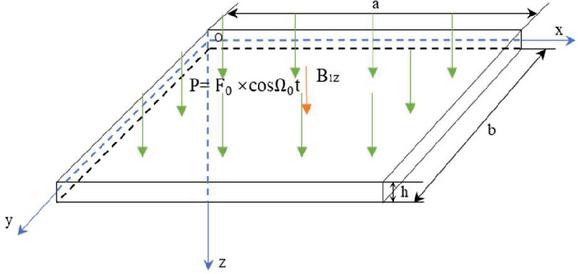
Figure 1 Model of a magnetoelastic rectangular sheet under mechanical excitation in a magnetic field environment.

This section makes the following four basic assumptions:

(1) Considering only displacement inertia forces and not rotational moments of inertia.

(2) The material of the sheet is considered to be linear elastic and isotropic in terms of its mechanical properties.

(3) No free charge, no current present in the material.

(4) Displacement of the midplane considering geometric nonlinear effects.

A Cartesian coordinate system is established on the mid-surface of a rectangular thin plate. Assume that the displacement of a point on the mid-surface is represented by $u$, $v$ and $w$ in the $x$, $y$ and $z$ directions, respectively.

According to the electromagnetic instanton relationship, for linear magnetized materials.

$$\{\begin{array}{c}\mathit{B}={\mu }_r{\mu }_0\mathit{H}\hfill \\ \mathit{M}={\chi }_m\mathit{H}\hfill \\ {\mu }_r=1+{\chi }_m\hfill \end{array}$$

(1)

Where $\mathit{M}$ is the magnetization vector, ${\mu }_0$ is the magnetic permeability in a vacuum, ${\mu }_r$ is the relative permeability, $\mathit{H}$ is the magnetic field strength vector, $\mathit{B}$ is the magnetic induction strength vector, $\mathit{J}=\mathit{B}\sigma \partial \mathit{u}/\partial t$ is the density vector, ${\chi }_m$ is the magnetic susceptibility, and $\sigma$ is the electrical conductivity.

According to the theory of elastic deformation, the displacement of the plate, whose internal distance from the midplane is $z$, can be expressed as follows:

$$\mathit{u}=\left[u_0(x,y)-z\frac{\partial w}{\partial x}\right]\mathit{i}+\left[v_0(x,y)-z\frac{\partial w}{\partial y}\right]\mathit{j}+w(x,y,t)\mathit{k}$$

(2)

In Equation (2), $\mathit{i},\mathit{j}$ and $\mathit{k}$ are unit vectors; $u_0$, $v_0$ and $w$ are the displacement components in the middle plane along the $x$, $y$, and $z$ axis directions.

Bringing Equation (2) into the expression for the Lorentzian electromagnetic force, we get:

$$=\sigma z\left(\mathit{i}{B}_{1z}^2\frac{{\partial }^{2}w}{\partial x\partial t}+\mathit{j}{B}_{z1}^2\frac{{\partial }^{2}w}{\partial y\partial t}\right)=f_x\mathit{i}+f_y\mathit{j}$$

(3)

The elastic deformation-induced equivalent magnetic force is:

$F_E={\displaystyle \frac{\partial }{\partial x}}{\displaystyle {\int }_{-\frac{h}{2}}^{\frac{h}{2}}}{f}_{x}z\mathit{d}z+{\displaystyle \frac{\partial }{\partial y}}{\displaystyle {\int }_{-\frac{h}{2}}^{\frac{h}{2}}}{f}_{y}z\mathit{d}z={\displaystyle \frac{\sigma h^3{B}_{1z}^2}{12}}\left({\displaystyle \frac{{\partial }^{3}w}{\partial x^2\partial t}}+{\displaystyle \frac{{\partial }^{3}w}{\partial y^2\partial t}}\right)$

(4)

Considering the distributed forces due to eddy currents at the mid-platen surface, using the magnetic dipole model [43] and neglecting the inertial forces in the surface, it is obtained that:

$$\begin{array}{cc}& \rho h\frac{{\partial }^{2}w}{\partial t^2}+D_M{\nabla }^{4}w\hfill \\ & -\frac{1}{2}{D}_N\left[{\left(\frac{\partial w}{\partial x}\right)}^2\frac{{\partial }^{2}w}{\partial x^2}+{\left(\frac{\partial w}{\partial y}\right)}^2\frac{{\partial }^{2}w}{\partial y^2}+2\frac{\partial w}{\partial x}\frac{\partial w}{\partial y}\frac{{\partial }^{2}w}{\partial x\partial y}\right]\hfill \\ & -\frac{{\chi }_m{B}_{1z}^2}{2{\mu }_r{\mu }_0}\left({\left(\frac{\partial w}{\partial x}\right)}^2+{\left(\frac{\partial w}{\partial y}\right)}^2\right)-\frac{\sigma h^3{B}_{1z}^2}{12}\left(\frac{{\partial }^{3}w}{\partial x^2\partial t}+\frac{{\partial }^{3}w}{\partial y^2\partial t}\right)\hfill \\ & =F_{0}cos{\mathrm{\Omega }}_{0}t\hfill \end{array}$$

(5)

$${\nabla }^4=\frac{{\partial }^4}{\partial x^4}+2\frac{{\partial }^4}{\partial x^2\partial y^2}+\frac{{\partial }^4}{\partial y^4}$$

(6)

In Equations (5) and (6), $\rho$ is the density of the rectangular thin plate; $D_M$ is the bending stiffness of the plate; $D_N$ is the tensile stiffness of the plate; $B_{1z}$ is the magnetic induction intensity; ${\nabla }^4$ is the dual Laplace operator;

From the condition of fixed three-sided simple support on one side of the rectangular sheet, the separation variable method is used so that the transverse displacement is [44]:

$$w=\sum _{n=1}^2{Q}_n(t)X_n(x)sin\frac{\pi y}{b}$$

(7)

In Equation (7)

$$X_n=cosh{\alpha }_{n}x-cos{\alpha }_{n}x-C_n(sinh{\alpha }_{n}x-sin{\alpha }_{n}x)$$

$$C_n=\frac{cosh{\alpha }_{n}a+cos{\alpha }_{n}a}{sinh{\alpha }_{n}a+sin{\alpha }_{n}a}$$

$${\alpha }_n=\frac{(4n+1)\pi }{4a}$$

Substitute Equations (6) and (7) into Equation (5):

$\rho h{\displaystyle \sum _{n=1}^2}sin{\displaystyle \frac{\pi y}{b}}{X}_n\ddot{Q_n}$
$\mathrm{\hspace{1em}\hspace{1em}}+D_M\left[\begin{array}{c}{\displaystyle \sum _{n=1}^2}sin{\displaystyle \frac{\pi y}{b}}X_n{}^{\left(4\right)}{Q}_n-{\left({\displaystyle \frac{\pi }{b}}\right)}^2{\displaystyle \sum _{n=1}^2}sin{\displaystyle \frac{\pi y}{b}}\ddot{X_n}{Q}_n\hfill \\ +{\left({\displaystyle \frac{\pi }{b}}\right)}^4{\displaystyle \sum _{n=1}^2}sin{\displaystyle \frac{\pi y}{b}}{X}_n{Q}_n\hfill \end{array}\right]$
$\mathrm{\hspace{1em}\hspace{1em}}-{\displaystyle \frac{1}{2}}{D}_N\left\{\begin{array}{c}{\left[{\displaystyle \sum _{n=1}^2}sin{\displaystyle \frac{\pi y}{b}}\dot{X_n}{Q}_n\right]}^2\left[{\displaystyle \sum _{n=1}^2}sin{\displaystyle \frac{\pi y}{b}}\ddot{X_n}{Q}_n\right]\hfill \\ -{\left({\displaystyle \frac{\pi }{b}}\right)}^2{\left[{\displaystyle \sum _{n=1}^2}cos{\displaystyle \frac{\pi y}{b}}{X}_n{Q}_n\right]}^2\hfill \\ \times \left[{\left({\displaystyle \frac{\pi }{b}}\right)}^2{\displaystyle \sum _{n=1}^2}sin{\displaystyle \frac{\pi y}{b}}{X}_n{Q}_n\right]\hfill \\ +2{\left({\displaystyle \frac{\pi }{b}}\right)}^2{\displaystyle \sum _{n=1}^2}sin{\displaystyle \frac{\pi y}{b}}\dot{X_n}{Q}_n{\displaystyle \sum _{n=1}^2}cos{\displaystyle \frac{\pi y}{b}}{X}_n{Q}_n\hfill \\ \times {\displaystyle \sum _{n=1}^2}cos{\displaystyle \frac{\pi y}{b}}\dot{X_n}{Q}_n\hfill \end{array}\right\}$
$\mathrm{\hspace{1em}\hspace{1em}}-{\displaystyle \frac{{\chi }_m{B}_{1z}^2}{2{\mu }_r{\mu }_0}}\left\{{\left[{\displaystyle \sum _{n=1}^2}sin{\displaystyle \frac{\pi y}{b}}\dot{X_n}{Q}_n\right]}^2+{\left({\displaystyle \frac{\pi }{b}}\right)}^2{\left[{\displaystyle \sum _{n=1}^2}sin{\displaystyle \frac{\pi y}{b}}{X}_n{Q}_n\right]}^2\right\}$
$\mathrm{\hspace{1em}\hspace{1em}}-{\displaystyle \frac{\sigma h^3{B}_{1z}^2}{12}}\left\{\left[{\displaystyle \sum _{n=1}^2}sin{\displaystyle \frac{\pi y}{b}}\ddot{X_n}\dot{Q_n}\right]-\left[{\left({\displaystyle \frac{\pi }{b}}\right)}^2{\displaystyle \sum _{n=1}^2}sin{\displaystyle \frac{\pi y}{b}}{X}_n\dot{Q_n}\right]\right\}$
$\mathrm{\hspace{1em}}=F_{0}cos{\mathrm{\Omega }}_{0}t$	(8)

Using the Galerkin’s method [45], the differential equation of the system is obtained as Equation (9).

The dimensionless treatment of Equation (9) reduces the system equation of motion to the Equations (10) and (11).

For the parameters in the Equations (9)–(11), see Appendix A and Appendix B for details.

${\displaystyle \frac{\rho hb}{2}}{\displaystyle \sum _{n=1}^2}{A}_{ni}\ddot{Q_n}+D_M{\displaystyle \sum _{n=1}^2}\left[{\displaystyle \frac{b}{2}}{M}_{ni}-{\displaystyle \frac{{\pi }^2}{b}}{C}_{ni}+{\displaystyle \frac{{\pi }^4}{2b^3}}{A}_{ni}\right]Q_n$
$-{\displaystyle \frac{D_N}{2}}\left\{\begin{array}{c}{\displaystyle \sum _{n=1}^2}\left({\displaystyle \frac{{\pi }^2}{4b}}{B}_{ni}-{\displaystyle \frac{{\pi }^4}{8b^3}}{H}_{ni}+{\displaystyle \frac{3b}{8}}{F}_{ni}\right)Q_n{}^3\hfill \\ +\left[{\displaystyle \frac{3b}{8}}\left(S_{2i}+2K_{2i}\right)-{\displaystyle \frac{3{\pi }^4}{8b^3}}{P}_{1i}+{\displaystyle \frac{{\pi }^2}{4b}}\left(S_{1i}+2K_{1i}\right)\right]Q_{1}Q_2{}^2\hfill \\ +\left[{\displaystyle \frac{3b}{8}}\left(S_{4i}+2K_{4i}\right)-{\displaystyle \frac{3{\pi }^4}{8b^3}}{P}_{2i}+{\displaystyle \frac{{\pi }^2}{4b}}\left(S_{3i}+2K_{3i}\right)\right]Q_1{}^2{Q}_2\hfill \end{array}\right\}$
$-{\displaystyle \frac{{\chi }_m{B}_{1z}^2}{2{\mu }_r{\mu }_0}}{\displaystyle \sum _{n=1}^2}\left[\left({\displaystyle \frac{4b}{3\pi }}{E}_{ni}+{\displaystyle \frac{4}{3b}}{R}_{ni}\right)Q_n{}^2+\left({\displaystyle \frac{8b}{3\pi }}{Y}_{1i}+{\displaystyle \frac{8}{3b}}{Y}_{2i}\right)Q_1{Q}_2\right]$
$-{\displaystyle \frac{\sigma b{h}^3{B}_{1z}^2}{24}}{\displaystyle \sum _{n=1}^2}\left[C_{ni}-{\left({\displaystyle \frac{\pi }{b}}\right)}^2{A}_{ni}\right]\dot{Q_n}={\displaystyle \frac{2b}{\pi }}{O}_i{F}_{0}cos{\mathrm{\Omega }}_{0}t$	(9)
$\begin{array}{cc}\hfill \ddot{q_1}(\tau )+{\omega }_1^2{q}_1(\tau )& =-g_1{q}_2(\tau )+{\mathit{c}}_{11}\dot{q_1}(\tau )+{\mathit{c}}_{21}\dot{q_2}(\tau )+{\eta }_{11}{q}_1^3(\tau )\hfill \\ & +{\eta }_{21}{q}_2^3(\tau )+{\mathcal{𝒮}}_{11}{q}_1(\tau )q_2^2(\tau )+{\mathcal{𝒮}}_{12}{q}_1^2(\tau )q_2(\tau )\hfill \\ & +{\varsigma }_{11}{q}_1^2(\tau )+{\varsigma }_{21}{q}_2^2(\tau )+q_1(\tau )q_2(\tau )+f_{1}cos\mathrm{\Omega }\tau \hfill \end{array}$	(10)
$\begin{array}{cc}\hfill \ddot{q_2}(\tau )+{\omega }_2^2{q}_2(\tau )& =-g_2{q}_1(\tau )+{\mathit{c}}_{22}\dot{q_2}(\tau )+{\mathit{c}}_{12}\dot{q_1}(\tau )+{\eta }_{22}{q}_2^3(\tau )\hfill \\ & +{\eta }_{12}{q}_1^3(\tau )+{\mathcal{𝒮}}_{21}{q}_1(\tau )q_2^2(\tau )+{\mathcal{𝒮}}_{22}{q}_1^2(\tau )q_2(\tau )\hfill \\ & +{\varsigma }_{12}{q}_1^2(\tau )+{\varsigma }_{22}{q}_2^2(\tau )+{\psi }_{12}{q}_1(\tau )q_2(\tau )+f_{2}cos\mathrm{\Omega }\tau \hfill \end{array}$	(11)

3 Multiscale Method for Solving the System

When solving the weakly nonlinear system using the multiscale method, introducing the small parameter $\epsilon (0<\epsilon \ll 1)$ into Equations (10) and (11), we get:

$\ddot{q_1}(\tau )+{\omega }_1^2{q}_1(\tau )$	$=-\epsilon \widetilde{g_1}{q}_2(\tau )+\epsilon {\tilde{\mathit{c}}}_{11}\dot{q_1}(\tau )+\epsilon {\tilde{\mathit{c}}}_{21}\dot{q_2}(\tau )$
	$\mathrm{\hspace{1em}}+\epsilon [{\tilde{\varsigma }}_{11}{q}_1^2(\tau )+{\tilde{\varsigma }}_{21}{q}_2^2(\tau )+{\tilde{\psi }}_{11}{q}_1(\tau )q_2(\tau )]+\epsilon {\tilde{f}}_{1}cos\mathrm{\Omega }\tau$
	$\mathrm{\hspace{1em}}+\epsilon [{\tilde{\eta }}_{11}{q}_1^3(\tau )+{\tilde{\eta }}_{21}{q}_2^3(\tau )+{\widetilde{\mathcal{𝒮}}}_{11}{q}_1(\tau )q_2^2(\tau )$
	$\mathrm{\hspace{1em}}+{\widetilde{\mathcal{𝒮}}}_{12}{q}_1^2(\tau )q_2(\tau )]$	(12)
$\ddot{q_2}(\tau )+{\omega }_2^2{q}_2(\tau )$	$=-\epsilon \widetilde{g_2}{q}_1(\tau )+\epsilon {\tilde{\mathit{c}}}_{22}\dot{q_2}(\tau )+\epsilon {\tilde{\mathit{c}}}_{12}\dot{q_1}(\tau )$
	$\mathrm{\hspace{1em}}+\epsilon [{\tilde{\varsigma }}_{12}{q}_1^2(\tau )+{\tilde{\varsigma }}_{22}{q}_2^2(\tau )+{\tilde{\psi }}_{12}{q}_1(\tau )q_2(\tau )]+\epsilon {\tilde{f}}_{2}cos\mathrm{\Omega }\tau$
	$\mathrm{\hspace{1em}}+\epsilon [{\tilde{\eta }}_{22}{q}_2^3(\tau )+{\tilde{\eta }}_{12}{q}_1^3(\tau )+{\widetilde{\mathcal{𝒮}}}_{21}{q}_1(\tau )q_2^2(\tau )$
	$\mathrm{\hspace{1em}}+{\widetilde{\mathcal{𝒮}}}_{22}{q}_1^2(\tau )q_2(\tau )]$	(13)

Among them, $\widetilde{g_1}=\frac{g_1}{\epsilon }$, $\widetilde{g_2}=\frac{g_2}{\epsilon }$, ${\tilde{\mathit{c}}}_{ij}=\frac{{\mathit{c}}_{ij}}{\epsilon }$, ${\tilde{\eta }}_{ij}=\frac{{\eta }_{ij}}{\epsilon }$, ${\widetilde{\mathcal{𝒮}}}_{ij}=\frac{{\mathcal{𝒮}}_{ij}}{\epsilon }$, ${\tilde{\varsigma }}_{ij}=\frac{{\varsigma }_{ij}}{\epsilon }$, ${\tilde{\psi }}_{11}=\frac{{\psi }_{11}}{\epsilon }$, ${\tilde{\psi }}_{12}=\frac{{\psi }_{12}}{\epsilon }$, ${\tilde{f}}_i=\frac{f_i}{\epsilon }$ $(i=1,2;j=1,2)$.

Suppose the solutions of Equations (12) and (13) are of the form [42]:

$q_1$	$=q_{11}(T_0,T_1)+\epsilon q_{12}(T_0,T_1)$	(14)
$q_2$	$=q_{21}(T_0,T_1)+\epsilon q_{22}(T_0,T_1)$	(15)

We let $T_{\mathrm{n}}={\epsilon }^n\tau (n=0,1)$, where $T_{\mathrm{n}}$ are the different scale time variables.

Bringing Equations (14), (15) into Equations (12), (13):

$[D_0^2+2\epsilon D_0{D}_1](q_{11}+\epsilon q_{12})+{\omega }_1^2(q_{11}+\epsilon q_{12})$
$\mathrm{\hspace{1em}\hspace{1em}}=-\epsilon \widetilde{g_1}(q_{21}+\epsilon q_{22})+\epsilon {\tilde{\mathit{c}}}_{11}(D_0+\epsilon D_1)(q_{11}+\epsilon q_{12})$
$\mathrm{\hspace{1em}\hspace{1em}}\mathit{\hspace{1em}}+\epsilon {\tilde{\mathit{c}}}_{21}(D_0+\epsilon D_1)(q_{21}+\epsilon q_{22})+\epsilon {\tilde{\eta }}_{11}{(q_{11}+\epsilon q_{12})}^3$
$\mathrm{\hspace{1em}\hspace{1em}}\mathit{\hspace{1em}}+\epsilon {\tilde{\eta }}_{21}{(q_{21}+\epsilon q_{22})}^3+\epsilon {\widetilde{\mathcal{𝒮}}}_{11}(q_{11}+\epsilon q_{12}){(q_{21}+\epsilon q_{22})}^2$
$\mathrm{\hspace{1em}\hspace{1em}}\mathit{\hspace{1em}}+\epsilon {\widetilde{\mathcal{𝒮}}}_{12}{(q_{11}+\epsilon q_{12})}^2(q_{21}+\epsilon q_{22})+\epsilon {\tilde{\varsigma }}_{11}{(q_{11}+\epsilon q_{12})}^2$
$\mathrm{\hspace{1em}\hspace{1em}}\mathit{\hspace{1em}}+\epsilon {\tilde{\varsigma }}_{21}{(q_{21}+\epsilon q_{22})}^2+\epsilon {\tilde{\psi }}_{11}(q_{11}+\epsilon q_{12})(q_{21}+\epsilon q_{22})+\epsilon {\tilde{f}}_{1}cos\mathrm{\Omega }\tau$	(16)
$[D_0^2+2\epsilon D_0{D}_1](q_{11}+\epsilon q_{12})+{\omega }_1^2(q_{11}+\epsilon q_{12})$
$\mathrm{\hspace{1em}\hspace{1em}}=-\epsilon \widetilde{g_1}(q_{21}+\epsilon q_{22})+\epsilon {\tilde{\mathit{c}}}_{11}(D_0+\epsilon D_1)(q_{11}+\epsilon q_{12})$
$\mathrm{\hspace{1em}\hspace{1em}}\mathit{\hspace{1em}}+\epsilon {\tilde{\mathit{c}}}_{21}(D_0+\epsilon D_1)(q_{21}+\epsilon q_{22})+\epsilon {\tilde{\eta }}_{11}{(q_{11}+\epsilon q_{12})}^3$
$\mathrm{\hspace{1em}\hspace{1em}}\mathit{\hspace{1em}}+\epsilon {\tilde{\eta }}_{21}{(q_{21}+\epsilon q_{22})}^3+\epsilon {\widetilde{\mathcal{𝒮}}}_{11}(q_{11}+\epsilon q_{12}){(q_{21}+\epsilon q_{22})}^2$
$\mathrm{\hspace{1em}\hspace{1em}}\mathit{\hspace{1em}}+\epsilon {\widetilde{\mathcal{𝒮}}}_{12}{(q_{11}+\epsilon q_{12})}^2(q_{21}+\epsilon q_{22})+\epsilon {\tilde{\varsigma }}_{11}{(q_{11}+\epsilon q_{12})}^2$
$\mathrm{\hspace{1em}\hspace{1em}}\mathit{\hspace{1em}}+\epsilon {\tilde{\varsigma }}_{21}{(q_{21}+\epsilon q_{22})}^2+\epsilon {\tilde{\psi }}_{11}(q_{11}+\epsilon q_{12})(q_{21}+\epsilon q_{22})$
$\mathrm{\hspace{1em}\hspace{1em}}\mathit{\hspace{1em}}+\epsilon {\tilde{f}}_{1}cos\mathrm{\Omega }\tau$	(17)

Expanded so that the coefficient of the same power of $\epsilon$ is zero.

For the terms of ${\epsilon }^0$:

$D_0^2{q}_{11}+{\omega }_1^2{q}_{11}$	$=0$	(18)
$D_0^2{q}_{21}+{\omega }_2^2{q}_{21}$	$=0$	(19)

For the terms of $\epsilon$:

$D_0^2{q}_{12}+{\omega }_1^2{q}_{12}$	$=-2D_0{D}_1{q}_{11}-\widetilde{g_1}{q}_{21}+{\tilde{\mathit{c}}}_{11}{D}_0{q}_{11}+{\tilde{\mathit{c}}}_{21}{D}_0{q}_{21}$
	$\mathrm{\hspace{1em}}+{\tilde{\eta }}_{11}{q}_{11}^3+{\tilde{\eta }}_{21}{q}_{21}^3+{\widetilde{\mathcal{𝒮}}}_{11}{q}_{11}{q}_{21}^2+{\widetilde{\mathcal{𝒮}}}_{12}{q}_{21}{q}_{11}^2$
	$\mathrm{\hspace{1em}}+{\tilde{\varsigma }}_{11}{q}_{11}^2+{\tilde{\varsigma }}_{21}{q}_{21}^2+{\tilde{\psi }}_{11}{q}_{11}{q}_{21}+{\tilde{f}}_{1}cos\mathrm{\Omega }\tau$	(20)
$D_0^2{q}_{22}+{\omega }_2^2{q}_{22}$	$=-2D_0{D}_1{q}_{21}-{\tilde{g}}_2^2{q}_{11}+{\tilde{\mathit{c}}}_{12}{D}_0{q}_{11}+{\tilde{\mathit{c}}}_{22}{D}_0{q}_{21}$
	$\mathrm{\hspace{1em}}+{\tilde{\eta }}_{12}{q}_{11}^3+{\tilde{\eta }}_{22}{q}_{21}^3+{\widetilde{\mathcal{𝒮}}}_{21}{q}_{11}{q}_{21}^2+{\widetilde{\mathcal{𝒮}}}_{22}{q}_{21}{q}_{11}^2$
	$\mathrm{\hspace{1em}}+{\tilde{\varsigma }}_{12}{q}_{11}^2+{\tilde{\varsigma }}_{22}{q}_{21}^2+{\tilde{\psi }}_{12}{q}_{11}{q}_{21}+{\tilde{f}}_{2}cos\mathrm{\Omega }\tau$	(21)

The terms of ${\epsilon }^0$ are written in complex form:

$q_{11}$	$=A_1(T_1)exp(i{\omega }_1{T}_0)+\overline{A_1}(T_1)exp(-i{\omega }_1{T}_0)$	(22)
$q_{21}$	$=A_2(T_1)exp(i{\omega }_2{T}_0)+\overline{A_2}(T_1)exp(-i{\omega }_2{T}_0)$	(23)

Where $A_1$ and $A_2$ are the complex functions to be determined, and $\overline{A_1}$ and $\overline{A_2}$ are their corresponding conjugate complex numbers. Substituting Equations (22), (23) into Equations (20), (21), we obtain:

$D_0^2{q}_{12}+{\omega }_1^2{q}_{12}$	$=(-2i{\omega }_1{A}_1^{\prime }+i{\omega }_1{\tilde{\mathit{c}}}_{11}{A}_1+3{\tilde{\eta }}_{11}{A}_1^2\overline{A_1}$
	$\mathrm{\hspace{1em}}+2{\widetilde{\mathcal{𝒮}}}_{11}{A}_1{A}_2\overline{A_2})exp(i{\omega }_1{T}_0)$
	$\mathrm{\hspace{1em}}+(-\widetilde{g_1}{A}_2+i{\omega }_2{\tilde{\mathit{c}}}_{21}{A}_2+3{\tilde{\eta }}_{21}{A}_2^2\overline{A_2}$
	$\mathrm{\hspace{1em}}+2{\widetilde{\mathcal{𝒮}}}_{12}{A}_1{A}_2\overline{A_1})exp(i{\omega }_2{T}_0)+\tilde{\eta }{}_{11}A{}^3{}_{1}exp(3i{\omega }_1{T}_0)$
	$\mathrm{\hspace{1em}}+{\tilde{\eta }}_{21}{A}_2^{3}exp(3i{\omega }_2{T}_0)+{\widetilde{\mathcal{𝒮}}}_{11}{A}_1{A}_2^{2}exp[i({\omega }_1+2{\omega }_2)T_0]$
	$\mathrm{\hspace{1em}}+{\widetilde{\mathcal{𝒮}}}_{11}{A}_1{\overline{A_2}}^{2}exp[i({\omega }_1-2{\omega }_2)T_0]$
	$\mathrm{\hspace{1em}}+{\widetilde{\mathcal{𝒮}}}_{12}{A}_1^2{A}_{2}exp[i(2{\omega }_1+{\omega }_2)T_0]$
	$\mathrm{\hspace{1em}}+{\widetilde{\mathcal{𝒮}}}_{12}{A}_2{\overline{A_1}}^{2}exp[i({\omega }_2-2{\omega }_1)T_0]$
	$\mathrm{\hspace{1em}}+{\widetilde{\mathcal{𝒮}}}_{11}{A}_2^2\overline{A_1}exp[i(2{\omega }_2-{\omega }_1)T_0]$
	$\mathrm{\hspace{1em}}+{\widetilde{\mathcal{𝒮}}}_{12}{A}_1^2\overline{A_2}exp[i(2{\omega }_1-{\omega }_2)T_0]+{\tilde{\varsigma }}_{11}{A}_{1}exp(2i{\omega }_1{T}_0)$
	$\mathrm{\hspace{1em}}+{\tilde{\varsigma }}_{21}{A}_{2}exp(2i{\omega }_2{T}_0)+{\tilde{\psi }}_{11}{A}_1{A}_{2}exp[i({\omega }_1+{\omega }_2)T_0]$
	$\mathrm{\hspace{1em}}+{\tilde{\psi }}_{11}\overline{A_1}{A}_{2}exp[i({\omega }_2-{\omega }_1)T_0]+0.5{\tilde{f}}_{1}exp(i\mathrm{\Omega }\tau )+cc$	(24)
$D_0^2{q}_{22}+{\omega }_1^2{q}_{22}$	$=(-2i{\omega }_2{A}_2^{\prime }+i{\omega }_2{\tilde{\mathit{c}}}_{22}{A}_2+3{\tilde{\eta }}_{22}{A}_2^2\overline{A_2}$
	$\mathrm{\hspace{1em}}+2{\widetilde{\mathcal{𝒮}}}_{22}{A}_1{A}_2\overline{A_1})exp(i{\omega }_2{T}_0)$
	$\mathrm{\hspace{1em}}+(-{\tilde{g}}_2^2{A}_1+i{\omega }_1{\tilde{\mathit{c}}}_{12}{A}_1+3{\tilde{\eta }}_{12}{A}_1^2\overline{A_1}$
	$\mathrm{\hspace{1em}}+2{\widetilde{\mathcal{𝒮}}}_{12}{A}_1{A}_2\overline{A_2})exp(i{\omega }_1{T}_0)+\tilde{\eta }{}_{22}A{}^3{}_{2}exp(3i{\omega }_2{T}_0)$
	$\mathrm{\hspace{1em}}+{\tilde{\eta }}_{12}{A}_1^{3}exp(3i{\omega }_1{T}_0)+{\widetilde{\mathcal{𝒮}}}_{22}{A}_2{A}_1^{2}exp[i({\omega }_2+2{\omega }_1)T_0]$
	$\mathrm{\hspace{1em}}+{\widetilde{\mathcal{𝒮}}}_{22}{A}_2{\overline{A_1}}^{2}exp[i({\omega }_2-2{\omega }_1)T_0]$
	$\mathrm{\hspace{1em}}+{\widetilde{\mathcal{𝒮}}}_{21}{A}_2^2{A}_{1}exp[i(2{\omega }_2+{\omega }_1)T_0]$
	$\mathrm{\hspace{1em}}+{\widetilde{\mathcal{𝒮}}}_{21}{A}_1{\overline{A_2}}^{2}exp[i({\omega }_1-2{\omega }_2)T_0]$
	$\mathrm{\hspace{1em}}+{\widetilde{\mathcal{𝒮}}}_{22}{A}_1^2\overline{A_2}exp[i(2{\omega }_1-{\omega }_2)T_0]$
	$\mathrm{\hspace{1em}}+{\widetilde{\mathcal{𝒮}}}_{21}{A}_2^2\overline{A_1}exp[i(2{\omega }_2-{\omega }_1)T_0]+{\tilde{\varsigma }}_{12}{A}_{1}exp(2i{\omega }_1{T}_0)$
	$\mathrm{\hspace{1em}}+{\tilde{\varsigma }}_{22}{A}_{2}exp(2i{\omega }_2{T}_0)+{\tilde{\psi }}_{12}{A}_1{A}_{2}exp[i({\omega }_1+{\omega }_2)T_0]$
	$\mathrm{\hspace{1em}}+{\tilde{\psi }}_{12}{A}_1\overline{A_2}exp[i({\omega }_1-{\omega }_2)T_0]$
	$\mathrm{\hspace{1em}}+{\tilde{\psi }}_{12}\overline{A_1}exp[i({\omega }_2-{\omega }_1)T_0]+{\displaystyle \frac{1}{2}}{\tilde{f}}_{2}exp\mathrm{?}(i\mathrm{\Omega }\tau )+cc$

In Equations (24), (3.14) $cc$ denotes the conjugate complex of the previous terms, and $A_1^{\prime }$ and $A_2^{\prime }$ denote the derivatives of $A_1$ and $A_2$ with respect to $T_1$.

If between two mode intrinsic frequencies, ${\omega }_2=3{\omega }_1$ is satisfied, then there is a 1:3 resonance phenomenon. Let the difference between ${\omega }_2$ and $3{\omega }_1$ be a small quantity of the same order of $\epsilon$ and introduce the coordination parameter ${\sigma }_1$, then [46]:

$${\omega }_2=3{\omega }_1+\epsilon {\sigma }_1$$

(26)

4 Principal and Internal Resonance

When the frequency $\mathrm{\Omega }$ of the dimensionless simple harmonic force approaches the system intrinsic frequency ${\omega }_1$, the system undergoes a first-order principal and internal resonance. To represent the relationship between the frequency of the simple harmonic force and the intrinsic frequency of the system, let the difference between ${\omega }_1$ and $\mathrm{\Omega }$ be a small quantity of the same order of $\epsilon$, and introduces the coordination parameter ${\sigma }_2$, then:

$$\mathrm{\Omega }={\omega }_1+\epsilon {\sigma }_2$$

(27)

Equations (26), (27) lead to the condition that $q_{12}$ and $q_{22}$ eliminate the permanent term as:

$-2i{\omega }_1{A}_1^{\prime }+i{\omega }_1{\tilde{\mathit{c}}}_{11}{A}_1+3{\tilde{\eta }}_{11}{A}_1^2\overline{A_1}+2{\widetilde{\mathcal{𝒮}}}_{11}{A}_1{A}_2\overline{A_2}$
$\mathrm{\hspace{1em}\hspace{1em}}+{\widetilde{\mathcal{𝒮}}}_{12}{A}_2{\overline{A_1}}^{2}exp(i{\sigma }_1{T}_1)+0.5{\tilde{f}}_{1}exp(i{\sigma }_2{T}_1)=0$	(28)
$-2i{\omega }_2{A}_2^{\prime }+i{\omega }_2{\tilde{\mathit{c}}}_{22}{A}_2+3{\tilde{\eta }}_{22}{A}_2^2\overline{A_2}+2{\widetilde{\mathcal{𝒮}}}_{22}{A}_1{A}_2\overline{A_1}$
$\mathrm{\hspace{1em}\hspace{1em}}+{\tilde{\eta }}_{12}{A}_1^{3}exp(-i{\sigma }_1{T}_1)=0$	(29)

From Equations (28), (29), it can be seen that there is no weakening trend of both $A_1$ and $A_2$. The first-order mode $A_1$ is associated with the simple harmonic force and generates the main resonance. The second-order mode is an internal indirect excitation due to the main resonance generated by the first-order mode.

Assumptions:

$$A_k=\frac{1}{2}{a}_k(T_1)exp[i{\theta }_k(T_1)]\mathit{\hspace{1em}}(k=1,2)$$

(30)

Substituting Equation (30) into Equations (28), (29), further separates the real part from the imaginary part [33]:

$$8{\omega }_1{a}_1^{\prime }=4{\omega }_1{\tilde{\mathit{c}}}_{11}{a}_1+{\widetilde{\mathcal{𝒮}}}_{12}{a}_1^2{a}_{2}sin{\beta }_1+4{\tilde{f}}_{1}sin{\beta }_2$$	(31)
$$8{\omega }_2{a}_2^{\prime }=4{\omega }_2{a}_2{\tilde{\mathit{c}}}_{22}-{\tilde{\eta }}_{12}{a}_1^{3}sin{\beta }_1$$	(32)
$$8{\omega }_1{\theta }_1^{\prime }{a}_1=-(3{\tilde{\eta }}_{11}{a}_1^2+2{\widetilde{\mathcal{𝒮}}}_{11}{a}_2^2)a_1-{\widetilde{\mathcal{𝒮}}}_{12}{a}_1^2{a}_{2}cos{\beta }_1-4{\tilde{f}}_{1}cos{\beta }_2$$	(33)
$$8{\omega }_2{\theta }_2^{\prime }{a}_2=-(3{\tilde{\eta }}_{22}{a}_2^2+2{\widetilde{\mathcal{𝒮}}}_{22}{a}_1^2)a_2-{\tilde{\eta }}_{12}{a}_1^{3}cos{\beta }_1$$	(34)

In Equations (31)–(34), ${\beta }_1={\theta }_2-3{\theta }_1+{\sigma }_1{T}_1$, ${\beta }_2={\sigma }_2{T}_1-{\theta }_1$.

$$4{\omega }_1{\tilde{\mathit{c}}}_{11}{a}_1+{\widetilde{\mathcal{𝒮}}}_{12}{a}_1^2{a}_{2}sin{\beta }_1+4{\tilde{f}}_{1}sin{\beta }_2=0$$	(35)
$$4{\omega }_2{a}_2{\tilde{\mathit{c}}}_{22}-{\tilde{\eta }}_{12}{a}_1^{3}sin{\beta }_1=0$$	(36)
$$(3{\tilde{\eta }}_{11}{a}_1^2+2{\widetilde{\mathcal{𝒮}}}_{11}{a}_2^2)a_1+{\widetilde{\mathcal{𝒮}}}_{12}{a}_1^2{a}_{2}cos{\beta }_1+4{\tilde{f}}_{1}cos{\beta }_2=8{\omega }_1{\sigma }_2{a}_1$$	(37)
$$(3{\tilde{\eta }}_{22}{a}_2^2+2{\widetilde{\mathcal{𝒮}}}_{22}{a}_1^2)a_2+{\tilde{\eta }}_{12}{a}_1^{3}cos{\beta }_1=8{\omega }_2{a}_2(3{\sigma }_2-{\sigma }_1)$$	(38)

Let $a_1\ne 0$, $a_2\ne 0$. The joint cubic Equations (35)–(38), eliminating ${\beta }_1$, ${\beta }_2$:

${[8{\omega }_2{a}_2(3{\sigma }_2-{\sigma }_1)+3{\tilde{\eta }}_{22}{a}_2^3+2{\widetilde{\mathcal{𝒮}}}_{22}{a}_1^2{a}_2]}^2+16{\omega }_2^2{a}_2^2{\tilde{\mathit{c}}}_{22}^2-{\tilde{\eta }}_{12}^2{a}_1^6=0$	(39)
$[2{\tilde{\eta }}_{12}{\omega }_1{\sigma }_2{a}_1^2+0.5({\tilde{\eta }}_{12}{\widetilde{\mathcal{𝒮}}}_{11}+{\widetilde{\mathcal{𝒮}}}_{12}{\widetilde{\mathcal{𝒮}}}_{22})a_1^2{a}_2^2+0.75{\tilde{\eta }}_{11}{\tilde{\eta }}_{12}{a}_1^4$
$\mathrm{\hspace{1em}}+3{\widetilde{\mathcal{𝒮}}}_{12}{\omega }_2{a}_2^2(3{\sigma }_2-{\sigma }_1)+0.75{\tilde{\eta }}_{22}{\widetilde{\mathcal{𝒮}}}_{12}{a}_2^4]$
$\mathrm{\hspace{1em}}+{({\tilde{\mathit{c}}}_{11}{\tilde{\eta }}_{12}{\omega }_1{a}_1^2+{\tilde{\mathit{c}}}_{22}{\widetilde{\mathcal{𝒮}}}_{12}{\omega }_2{a}_2^2)}^2-{\tilde{\eta }}_{12}^2{a}_1^2\widetilde{f_1^2}=0$	(40)

5 Example Analysis

From Equations (10), (11), ${\omega }_1=k_1/{\omega }_n=\sqrt{k_1/k_2}=1/{\omega }_2$, and the need to achieve 1:3 internal resonance requires that the value of ${\omega }_1/{\omega }_2$ is close to 1/3. Taking $b/a=2$, the condition can be satisfied [47]. The object of this study is a rectangular thin plate, whose material is soft ferromagnetic.

Parameter values [43]: Electrical conductivity $\sigma =2.3\times {10}^6{(\mathrm{\Omega }\cdot \mathrm{m})}^{-1}$, Material density $\rho =7800$ kg/m${}^3$, Poisson’s ratio $\mu =0.3$, Modulus of elasticity $E=2\times {10}^{11}$ Pa, $a=0.6$ m, $b=1.2$ m, $h=0.003$ m, Magnetization coefficient ${\chi }_m=1000$.

5.1 Amplitude-frequency Response Analysis

The amplitude-frequency characteristic curves at various magnetic field strengths for the simple harmonic force amplitude $F_0=25000$ N/m${}^2$ are shown in Figure 2. From Figure 2, it can be concluded that both modes are excited and the image curves show a complex phenomenon of multiple values and steps.

From Figure 2, it can be known that the number of steady-state solutions of the first-order and second-order modes is transformed from a single solution to multiple solutions when the magnetic field disturbance is ignored. When the magnetic field is considered, the resonance region of two modes becomes smaller and the maximum value of the resonance response also becomes smaller. This indicates that the magnetic field suppresses the resonance response of two modes.

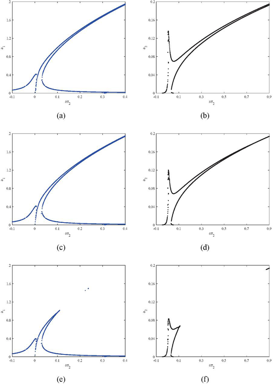
Figure 2 (a), (c) and (e) are the amplitude-frequency response curves of the first-order mode for magnetic induction strengths of 0T, 10T and 15T; (b), (d) and (f) are the amplitude-frequency response curves of the second-order mode for magnetic induction strengths of 0T, 10T and 15T.

5.2 Dynamic Response Analysis

The system of dimensionless differential Equations (10), (11) are solved using MATLAB software and programmed according to the Runge-Kutta method, at this time taking $\mathrm{\Omega }={\omega }_1+\epsilon {\sigma }_2=0.6$, $\epsilon {\sigma }_2=0.02$, ${\omega }_1=0.577$, ${\omega }_2=1.733$.

The waveforms, phase trajectory curves, and Poincaré scatter plots for two orders under the first-order principal and internal resonance with magnetic field strength $B_{1z}=0T$ and simple harmonic force amplitude $F_0=25000$ N/m${}^2$ are shown in Figure 3. Where (a), (c), (e) represent the first-order mode response, which is directly influenced by the simple harmonic force; (b), (d), (f) represent the second-order mode response, which is not directly influenced by the simple harmonic force, but by the internal resonance with the first-order mode, the energy of two modes is transferred, thus contributing to the indirect excitation. From the displacement time curve and phase trajectory diagram, it is obvious that the amplitude of the first-order mode is about 10 times of the second-order mode amplitude when $F_0=25000$ N/m${}^2$. This indicates that the resonance situation is dominated by the first-order mode at this point.

When the magnetic field strength $B_{1z}=0T$, the phase trajectory map of the first-order mode in Figure 3 presents a symmetric multiple limit-loop phase set, and the points of the Poincaré mapping are distributed on a closed curve with a quasi-periodic shape. The second-order mode, on the other hand, presents a shape of a center-symmetric irregular multiple limit-loop set, and the points on the image are a certain collection of scattered points, showing chaotic morphology, as can be seen from the Poincaré mapping of the second-order mode.

Figure 3 (a), (c) and (e) are the time displacement curve, phase trajectory, and Poincare map of the first-order mode with magnetic induction equal to 0T; (b), (d) and (f) are the time displacement curve, phase trajectory, and Poincare map of the second-order mode with magnetic induction equal to 0T.

Figure 4 (a), (c) and (e) are the time displacement curve, phase trajectory, and Poincare map of the first-order mode with magnetic induction equal to 2.5T; (b), (d) and (f) are the time displacement curve, phase trajectory, and Poincare map of the second-order mode with magnetic induction equal to 2.5T.

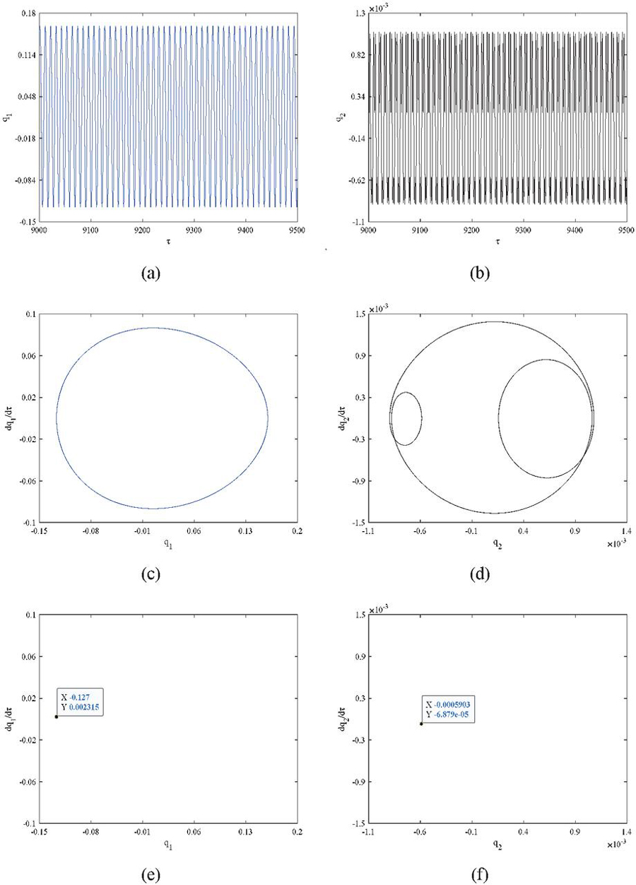
Figure 5 (a), (c) and (e) are the time displacement curve, phase trajectory, and Poincare map of the first-order mode with magnetic induction equal to 10T; (b), (d) and (f) are the time displacement curve, phase trajectory, and Poincare map of the second-order mode with magnetic induction equal to 10T.

The waveforms, phase trajectory curves and Poincaré scatter diagrams for two orders under the first-order principal and internal resonance for simple harmonic force amplitude $F_0=25000$ N/m${}^2$ are displayed in Figures 4 and 5. As can be known from Figure 5, when $B_{1z}=2.5T$, the points on two mode Poincaré scatter diagrams are distributed on a cyclic curve, which shows quasi-periodic form; The phase trajectory curve shows reciprocal motion. As shown in Figure 5, when $B_{1z}=10T$, the phase trajectory curve of two modes is a cyclic curve, while the Poincaré scatter plot is a point. This shows that the kinematic state of the system is affected when the system considers the magnetic field disturbance. The disturbance of the magnetic field will change with time, so that the modal state, which was in a chaotic or quasi-periodic state of motion, will eventually change to a stable periodic state of motion, and the response of the modal state will gradually disappear, with the magnetic field acting as a damping action.

6 Conclusion

This paper studies the nonlinear motion of a soft ferromagnetic rectangular thin plate under the action of a magnetic field. The equations of motion of the soft ferromagnetic rectangular thin plate are derived by considering the magnetic field effects under the coupling of magnetization and eddy currents. The control equations of two modes amplitude and phase of the system are accessed by the Galerkin’s method and multiscale method. The effect of the variation of the magnetic field on the system motion is further analyzed by numerical simulations. The results show that:

(1) The vibrational modes can interact with each other in resonant interactions. When the resonance is dominated by first-order modes, the first-order mode is influenced by the simple harmonic force. The second-order mode is then influenced by the first-order mode, which further generates the internal resonance phenomenon.

(2) The existence of internal resonance makes the system energy exchange between the two mutually coupled modes; the first two modes of the system are decayed by mutual coupling oscillation under the action of the magnetic field, and the decay rate is accelerated with the increase of magnetic field strength. The amplitude-frequency characteristic curves are accompanied by nonlinear phenomena such as multiple values and jumps; the magnetic field strength has a suppressive effect on the resonance amplitude.

(3) From the dynamic response, it is clear that the passage of time, without magnetic field disturbance, does not affect the kinematic state of the system. The mode in the main resonance will remain in a stable periodic motion, while the mode in the inner resonance will remain in a chaotic state. When the system considers the magnetic field disturbance, the resonance response of the system will be suppressed significantly, and the kinematic properties will reach a stable periodic kinematic state with time and the strengthening of the magnetic field. In practical engineering, the kinematic properties of the system can be changed by adjusting the magnetic field strength.

Acknowledgments

This research was funded by the Anhui Provincial Natural Science Foundation (Grant No. 2008085QE245), the Natural Science Research Project of Higher Education Institutions in Anhui Province (Grant No. 2022AH040045), the Project of Science and Technology Plan of Department of Housing and Urban-Rural Development of Anhui Province (Grant No. 2021-YF22), the National College Student Innovation and Entrepreneurship Training Program Project (Grant No. 202210878005).

Appendix A

The parameters in Equation (9) are given below:

$$A_{ni}={\int }_0^a{X}_n{X}_i\mathit{d}x,B_{ni}={\int }_0^a{\left(\frac{d{X}_n}{dx}\right)}^2{X}_n{X}_i\mathit{d}x,$$

$$C_{ni}={\int }_0^a\frac{d^2{X}_n}{d{x}^2}{X}_i\mathit{d}x,O_i={\int }_0^a{X}_i\mathit{d}x,M_{ni}={\int }_0^a\frac{d^4{X}_n}{d{x}^4}{X}_i\mathit{d}x,$$

$$F_{ni}={\int }_0^a\frac{d^2{X}_n}{d{x}^2}{\left(\frac{d{X}_n}{dx}\right)}^2{X}_i\mathit{d}x,H_{ni}={\int }_0^{a}X_n{}^3{X}_i\mathit{d}x,$$

$$P_{1i}={\int }_0^a{X}_{1}X_2{}^2{X}_i\mathit{d}x,P_{2i}={\int }_0^a{X}_{2}X_1{}^2{X}_i\mathit{d}x,$$

$$S_{1i}={\int }_0^a{X}_1{\left(\frac{d{X}_2}{dx}\right)}^2{X}_i\mathit{d}x,S_{2i}={\int }_0^a\frac{d^2{X}_1}{d{x}^2}{\left(\frac{d{X}_2}{dx}\right)}^2{X}_i\mathit{d}x,$$

$$S_{3i}={\int }_0^a{X}_2{\left(\frac{d{X}_1}{dx}\right)}^2{X}_i\mathit{d}x,S_{4i}={\int }_0^a\frac{d^2{X}_2}{d{x}^2}{\left(\frac{d{X}_1}{dx}\right)}^2{X}_i\mathit{d}x,$$

$$K_{1i}={\int }_0^a\frac{d{X}_1}{dx}\frac{d{X}_2}{dx}{X}_2{X}_i\mathit{d}x,K_{2i}={\int }_0^a\frac{d{X}_1}{dx}\frac{d{X}_2}{dx}\frac{d^2{X}_2}{d{x}^2}{X}_i\mathit{d}x,$$

$$K_{3i}={\int }_0^a\frac{d{X}_1}{dx}\frac{d{X}_2}{dx}{X}_1{X}_i\mathit{d}x,K_{4i}={\int }_0^a\frac{d{X}_1}{dx}\frac{d{X}_2}{dx}\frac{d^2{X}_1}{d{x}^2}{X}_i\mathit{d}x,$$

$$E_{ni}={\int }_0^a{\left(\frac{d{X}_n}{dx}\right)}^2{X}_i\mathit{d}x,R_{ni}={\int }_0^{a}X_n{}^2{X}_i\mathit{d}x,$$

$$Y_{1i}={\int }_0^a\frac{d{X}_1}{dx}\frac{d{X}_2}{dx}{X}_{i}dx,Y_{2i}={\int }_0^a{X}_1{X}_2{X}_{i}dx;(i=1,2;n=1,2)$$

Appendix B

The parameters in Equations (10), (11) are given below:

$$q_n=\frac{Q_n}{h},k_1^2=\frac{D_M{M}_{11}}{\rho h{A}_{11}}-\frac{2{\pi }^2{D}_M{C}_{11}}{\rho h{b}^2{A}_{11}}+\frac{{\pi }^4{D}_M}{b^4\rho h},$$

$$k_2^2=\frac{D_M{M}_{22}}{\rho h{A}_{22}}-\frac{2{\pi }^2{D}_M{C}_{22}}{\rho h{b}^2{A}_{22}}+\frac{{\pi }^4{D}_M}{b^4\rho h},$$

$${\omega }_n=\sqrt{k_1{k}_2},{\omega }_1=\frac{k_1}{{\omega }_n},{\omega }_2=\frac{k_2}{{\omega }_n},$$

$$f_1=\frac{4}{\pi \rho h{A}_{11}{\omega }_n^2}{O}_1{F}_0,f_2=\frac{4}{\pi \rho h{A}_{22}{\omega }_n^2}{O}_2{F}_0,$$

$$g_1=\frac{D_M{M}_{21}}{\rho h{A}_{11}{\omega }_n^2}-\frac{2{\pi }^2{D}_M{C}_{21}}{\rho h{b}^2{A}_{11}{\omega }_n^2}+\frac{{\pi }^4{D}_M{A}_{21}}{A_{11}{b}^4\rho h{\omega }_n^2},$$

$$g_2=\frac{D_M{M}_{12}}{\rho h{A}_{22}{\omega }_n^2}-\frac{2{\pi }^2{D}_M{C}_{12}}{\rho h{b}^2{A}_{22}{\omega }_n^2}+\frac{{\pi }^4{D}_M{A}_{12}}{A_{22}{b}^4\rho h{\omega }_n^2},$$

$$c_{11}=\frac{\sigma h^2{B}_{1z}^2}{12\rho {\omega }_n}\left[\frac{C_{11}}{A_{11}}-{\left(\frac{\pi }{b}\right)}^2\right],c_{22}=\frac{\sigma h^2{B}_{1z}^2}{12\rho {\omega }_n}\left[\frac{C_{22}}{A_{22}}-{\left(\frac{\pi }{b}\right)}^2\right],$$

$$c_{21}=\frac{\sigma h^2{B}_{1z}^2}{12\rho {\omega }_n}\left[\frac{C_{21}}{A_{11}}-{\left(\frac{\pi }{b}\right)}^2\right],c_{12}=\frac{\sigma h^2{B}_{1z}^2}{12\rho {\omega }_n}\left[\frac{C_{12}}{A_{22}}-{\left(\frac{\pi }{b}\right)}^2\right],$$

$$\tau ={\omega }_{n}t,\mathrm{\Omega }=\frac{{\mathrm{\Omega }}_0}{{\omega }_n},a_1=\frac{h{D}_N}{2\rho b{\omega }_n^2},a_2=\frac{{\chi }_m{B}_{1z}^2}{{\omega }_n^2\rho b{\mu }_r{\mu }_0},$$

$${\eta }_{11}=\frac{a_1}{A_{11}}\left(\frac{{\pi }^2}{4b}{B}_{11}-\frac{{\pi }^4}{8b^3}{H}_{11}+\frac{3b}{8}{F}_{11}\right),$$

$${\eta }_{21}=\frac{a_1}{A_{11}}\left(\frac{{\pi }^2}{4b}{B}_{21}-\frac{{\pi }^4}{8b^3}{H}_{21}+\frac{3b}{8}{F}_{21}\right),$$

$${\eta }_{22}=\frac{a_1}{A_{22}}\left(\frac{{\pi }^2}{4b}{B}_{22}-\frac{{\pi }^4}{8b^3}{H}_{22}+\frac{3b}{8}{F}_{22}\right),$$

$${\eta }_{12}=\frac{a_1}{A_{22}}\left(\frac{{\pi }^2}{4b}{B}_{12}-\frac{{\pi }^4}{8b^3}{H}_{12}+\frac{3b}{8}{F}_{12}\right),$$

$${\varsigma }_{11}=\frac{a_2}{A_{11}}\left(\frac{4b}{3\pi }{E}_{11}+\frac{4}{3b}{R}_{11}\right),{\varsigma }_{21}=\frac{a_2}{A_{11}}\left(\frac{4b}{3\pi }{E}_{21}+\frac{4}{3b}{R}_{21}\right),$$

$${\varsigma }_{22}=\frac{a_2}{A_{22}}\left(\frac{4b}{3\pi }{E}_{22}+\frac{4}{3b}{R}_{22}\right),{\varsigma }_{12}=\frac{a_2}{A_{22}}\left(\frac{4b}{3\pi }{E}_{12}+\frac{4}{3b}{R}_{12}\right),$$

$${\psi }_{11}=\frac{a_2}{A_{11}}\left(\frac{8b}{3\pi }{Y}_{11}+\frac{8}{3b}{Y}_{21}\right),{\psi }_{12}=\frac{a_2}{A_{22}}\left(\frac{8b}{3\pi }{Y}_{12}+\frac{8}{3b}{Y}_{22}\right),$$

$${\mathcal{𝒮}}_{11}=\frac{a_1}{A_{11}}\left[\frac{3b}{8}\left(S_{21}+2K_{21}\right)-\frac{3{\pi }^4}{8b^3}{P}_{11}+\frac{{\pi }^2}{4b}\left(S_{11}+2K_{11}\right)\right],$$

$${\mathcal{𝒮}}_{12}=\frac{a_1}{A_{11}}\left[\frac{3b}{8}\left(S_{41}+2K_{41}\right)-\frac{3{\pi }^4}{8b^3}{P}_{21}+\frac{{\pi }^2}{4b}\left(S_{31}+2K_{31}\right)\right],$$

$${\mathcal{𝒮}}_{21}=\frac{a_1}{A_{22}}\left[\frac{3b}{8}\left(S_{22}+2K_{22}\right)-\frac{3{\pi }^4}{8b^3}{P}_{12}+\frac{{\pi }^2}{4b}\left(S_{12}+2K_{12}\right)\right]$$

References

[1] M. A. Abazid, “The Nonlocal Strain Gradient Theory for Hygrothermo-Electromagnetic Effects on Buckling, Vibration and Wave Propagation in Piezoelectromagnetic Nanoplates,” International Journal of Applied Mechanics, vol. 11, no. 7, pp. 31, 2019.

[2] F. X. Duthoit, T. S. Hahm and L. Wang, “Electromagnetic nonlinear gyrokinetics with polarization drift,” Advanced Materials Research, vol. 21, no. 8, pp. 1–11, 2014.

[3] T. Rabenimanana, V. Walter and M. Kacem, “Functionalization of electrostatic nonlinearities to overcome mode aliasing limitations in the sensitivity of mass microsensors based on energy localization,” Applied Physics Letters, vol. 117, no. 3, pp. 6, 2020.

[4] T. C. Adorno, D. M. Gitman, A. E. Shabad and A. A. Shishmarev, “Quantum Electromagnetic Nonlinearity Affecting Charges and Dipole Moments,” Russian Physics Journal, vol. 59, no. 11, pp. 1775–1787, 2017.

[5] R. Y. Li, H. Q. Zhang, H. Q. Gao, Z. Wu and C. X. Guo, “An improved extreme learning machine algorithm for transient electromagnetic nonlinear inversion,” Computers & Geosciences, vol. 156, pp. 104877, 2021.

[6] V. Balasubramanian, A. Bernamonti, J. de Boer et al., “Inhomogeneous thermalization in strongly coupled field theories,” Physical Review B: Condensed Matter & Materials Physics, vol. 111, no. 23, pp. 231602, 2013.

[7] L. Cheng, Y. Yang, F. L. Jiang and C. Li, “Experimental investigation and FEM analysis of laser cladding assisted by coupled field of electric and magnetic,” Materials Research Express, vol. 6, no. 1, pp. 016516, 2019.

[8] Y. L. Lv, K. Guo, L. M. He, L. C. Shi and Y. Cao, “Effect of Frequency on Dehydration Efficiency under the Electromagnetic Coupling Field,” Journal of Chemical Engineering of Japan, vol. 53, no. 2, pp. 49–57, 2020.

[9] S. A. Zhou, “Magnetoelastic theory of type-II superconductors in the mixed state,” Physical Review, vol. 50, no. 1, pp. 354–361, 1994.

[10] O. Tsyplyatyev, P. Kopietz, Y. Tsui et al., “Many-body theory of magnetoelasticity in one dimension,” Physical Review B, vol. 95, no. 4, 2017.

[11] Z. Yin, H. D. Gao and G. Lin, “An efficient semi-analytical static and free vibration analysis of laminated and sandwich beams based on linear elasticity theory,” The Journal of Strain Analysis for Engineering Design, vol. 57, no. 8, pp. 631–646, 2022.

[12] S. B. Medvedev and V. N. Grebenev, “Hamiltonian structure and conservation laws of two-dimensional linear elasticity theory,” ZAMM - Journal of Applied Mathematics and Mechanics, vol. 96, no. 10, pp. 1175–1183, 2016.

[13] S. I. Kruglov, “Dyonic and magnetized black holes based on nonlinear electrodynamics,” European Physical Journal C: Particles and Fields, vol. 80, no. 3, 2020.

[14] B. K. Datta, “MagnetoElastic Wave Propagation in a Linear Viscoelastic Solid Medium,” Proceedings of Indian National Science Academy, vol. 52, no. 6A, 2015.

[15] D. V. Rastyagaev, E. A. Palkin, D. S. Lukin, A. S. Kryukovsky and E. V. Ipatov, “Application of the Diffraction-Ray Theory to the Problems of Propagation of Electromagnetic Waves in the Ionospheric Plasma,” Radiophysics and Quantum Electronics, vol. 64, no. 8–9, pp. 533–544, 2022.

[16] P. Bradley, “A dense voltage-mode Josephson memory cell insensitive to systematic variations in critical current density,” IEEE Transactions on Magnetics, vol. 21, no. 2, pp. 729–732, 1985.

[17] V. V. Fadin, M. I. Aleutdinova and O. A. Kulikova, “Average contact temperature and morphological details of the worn surface of copper based materials under high current density sliding against steel,” AIP Conference Proceedings, vol. 1783, no. 1, pp. 020051, 2016.

[18] W. P. Zhang, J. Y. Chen and X. J. Luo, “Effects of impressed current density on corrosion induced cracking of concrete cover,” Construction and Building Materials, vol. 204, pp. 213–223, 2019.

[19] M. Malikan, V. A. Eremeyev, “Flexomagnetic response of buckled piezomagnetic composite nanoplates,” Compos. Struct, vol. 267, pp. 113932, 2021.

[20] M. Malikan, V. A. Eremeyev, “On dynamic modeling of piezomagnetic flexoma-gnetic microstructures based on Lord–Shulman thermoelastic model,” Arch Appl Mech, vol. 93, pp. 181–196, 2023.

[21] M. Malikan, V. A. Eremeyev, “On a flexomagnetic behavior of composite structures,” Int J Eng Sci, vol. 175, pp. 103671, 2022.

[22] M. Malikan, V. A. Eremeyev, “Flexomagneticity in buckled shear deformable hard-magnetic soft structures,” Contin. Mech. Thermodyn, pp. 1–16, 2021.

[23] H. Altenbach, O. Morachkovsky, K. Naumenko and D. Lavinsky, “Inelastic deformation of conductive bodies in electromagnetic fields,” Continuum Mechanics and Thermodynam, vol. 28, no. 5, pp. 1421–1433, 2016.

[24] S. O. Gladkov, “Theory of Electromagnetic Radiation by Inertially Moving Conductive Bodies,” Journal of Communications Technology and Electronics, vol. 66, no. 6, pp. 690–693, 2021.

[25] T. J. Yin, X. J. Jiang and W. Qin, “A magnetic field-directed self-assembly solid contact for construction of an all-solid-state polymeric membrane Ca${}^{2+}$-selective electrode,” Analytica Chimica Acta, vol. 56, no. 989, pp. 15–20, 2017.

[26] M. Martinez-Santiesteban Francisco, D. Swanson Scott, C. Noll Douglas and J. Anderson David, “Magnetic field perturbation of neural recording and stimulating microelectrodes,” Physics in Medicine & Biology, vol. 52, no. 8, pp. 2073–2088, 2007.

[27] Y. Kim and X. H. Zhao, “Magnetic Soft Materials and Robots,” Chemical Reviews, vol. 122, no. 5, pp. 5317–5364, 2022.

[28] W. J. Yang, J. J. Liu, X. F. Yu et al., “The Preparation of High Saturation Magnetization and Low Coercivity Feco Soft Magnetic Thin Films via Controlling the Thickness and Deposition Temperature,” Materials, vol. 15, no. 20, pp. 7191–7191, 2022.

[29] J. W. Zheng, D. N. Zheng, L. Qiao et al., “High permeability and low core loss Fe-based soft magnetic composites with Co-Ba composite ferrite insulation layer obtained by sol-gel method,” Journal of Alloys and Compounds, vol. 893, 2022.

[30] Anil K. Bastola and Mokarram Hossain, “The shape – morphing performance of magnetoactive soft materials,” Materials & Design, vol. 893, pp. 110172, 2021.

[31] K. Niitsu, “Temperature dependence of magnetic exchange stiffness in iron and nickel,” Journal of Physics D: Applied Physics, vol. 53, no. 39, 2020.

[32] K. G. Suresh, R. Srinivasan, G. Karunakaran et al., “Microwave-assisted combustion synthesis of soft ferromagnetic spinel MFe${}_2$O${}_4$ (M $=$ Ni, Mg, Zn) nanoparticles using Citrus limon fruit extract as a fuel,” Applied Physics A, vol. 127, no. 7, 2021.

[33] E. Sobhani and M. Avcar, “Natural frequency analysis of imperfect GNPRN conical shell, cylindrical shell, and annular plate structures resting on Winkler-Pasternak Foundations under arbitrary boundary conditions,” Eng Anal Bound Elem, vol. 144, pp. 145–164, 2022.

[34] L. Hadji and M. Avcar, “Free Vibration Analysis of FG Porous Sandwich Plates under V-arious Boundary Conditions,” J. Appl. Comput. Mech, vol. 7, no. 2, pp. 505–519, 2021.

[35] O. Civalek and M. Avcar, “Free vibration and buckling analyses of CNT reinforced laminated non-rectangular plates by discrete singular convolution method,” Engineering with Computers, vol. 38, pp. 489–521, 2022.

[36] P. Van Vinh, M. Avcar, M. O. Belarbi et al., “A new higher-order mixed four-node quadrilateral finite element for static bending analysis of functionally graded plates,” Structures, vol. 47, pp. 1595–1612, 2023.

[37] A. Daikh, M. Belarbi, D. Ahmed et al., “Static analysis of functionally graded plate structures resting on variable elastic foundation under various boundary conditions,” Acta Mech, vol. 234, pp. 775–806, 2023.

[38] V. A. Krysko, A. Awrejcewicz and I. V. Papkova, “Chaotic vibrations of size-dependent flexible rectangular plates,” Chaos, vol. 31, no. 4, pp. 043119–043119, 2021.

[39] P. Li, Z. X. Wang, D. C. Zhang and Y. R. Yang, “On bifurcations and chaos of a forced rectangular plate with large deflection loaded by subsonic airflow,” Thin-Walled Structures, vol. 161, 2021.

[40] K. L. Wang and C. F. Wei, “New Analytical Approach for Nonlinear Fractal K(p,q) Model,” Fractals: Complex Geometry, Patterns, and Scaling in Nature and Society, vol. 29, no. 5, 2021.

[41] L. Ma, M. H. Yao, W. Zhang and D. X. Cao, “Bifurcation and dynamic behavior analysis of a rotating cantilever plate in subsonic airflow,” Applied Mathematics and Mechanics (English Edition), vol. 41, pp. 1–20, 2020.

[42] J. J. Qing, S. S. Zhou, J. M. Wu and M. Y. Shao, “Primary and secondary resonance responses of fractional viscoelastic PET membranes,” Communications in Nonlinear Science and Numerical Simulation, vol. 116, 2023.

[43] C. X. Xue, E. Pan, Q. K. Han, S. Y. Zhang and H. J. Chu, “Non-linear principal resonance of an orthotropic and magnetoelastic rectangular plate,” International Journal of Non-Linear Mechanics, vol. 46, no. 5, pp. 703–710, 2011.

[44] Z. Y. Cao and Y. H. Pao, “Vibration theory of plates and shells,” Beijing: China Railway Publishing House, 1983.

[45] J. Wang and R. X. Wu, “The Extended Galerkin Method for Approximate Solutions of Nonlinear Vibration Equations,” Applied sciences, vol. 12, no. 6, pp. 2979, 2022.

[46] A. H. Nayfeh and S. A. Emam, “Non-linear response of buckled beams to 1:1 and 3:1 internal resonances,” Int. J. Nonlin. Mech, vol. 52, pp. 12–25, 2013.

[47] J. Li and Y. D. Hu, “Principal and internal resonance of rectangular conductive thin plate in transverse magnetic field,” Theoretical & Applied Mechanics Letters, vol. 8, no. 4, pp. 257–266, 2018.

Biographies

Xiaofang Kang received the B.S. degree in Engineering Management from Anhui Jianzhu University, Hefei, China, in 2009 and the M.S. degree in Engineering Mechanics from Hefei University of Technology, Hefei, China, in 2012. He received the Ph.D. degree in Structural Engineering from Hefei University of Technology, Hefei, China, in 2016. He research interests include Structural vibration control and energy harvesting.

Xinzong Wang received the B.S. degree in Civil Engineering from Wuxi Taihu University, Wuxi, China, in 2019. He is currently working toward the M.S. degree in Structural Engineering with the School of Civil Engineering, Anhui Jianzhu University, Hefei, China. He research interests include Structural vibration control and Nonlinear Vibration Analysis.

Qingguan Lei received the B.S. degree in Water Resources and Hydropower Engineering from Hefei University of Technology, Hefei, China, in 1985 and the M.S. degree in Structural Engineering from Hefei University of Technology, Hefei, China, in 1991. He research interests include Structural vibration control and energy harvesting.

Zhengxing Zhu received the B.S. degree in Civil Engineering from Suzhou University, Suzhou, China, in 2020. He is currently working toward the M.S. degree in Structural Engineering with the School of Civil Engineering, Anhui Jianzhu University, Hefei, China. The main research direction is engineering disaster prevention and reduction.

Ziyi Sheng is currently working toward the B.S. degree in Civil Engineering with the School of Civil Engineering, Anhui Jianzhu University, Hefei, China. The main research direction is engineering disaster prevention and reduction.

Fuyi Zhang is currently studying for a bachelor’s degree in civil engineering at the School of Civil Engineering, Anhui Jianzhu University, Hefei, China. He mainly studies structural reliability and use safety. The main research direction is engineering disaster prevention and reduction.

European Journal of Computational Mechanics, Vol. 33_1, 1–30.
doi: 10.13052/ejcm2642-2085.3311
© 2024 River Publishers