The Influence of Spatially Varying Boundary Conditions Based on Material Heterogeneity
Evan John Ricketts1,*, Peter John Cleall1, Anthony Jefferson1, Pierre Kerfriden2 and Paul Lyons3
1School of Engineering, Cardiff University, Cardiff, CF24 3AA, UK
2Centre de Matériaux, Mines Paris /PSL University, Evry, France
3LUSAS, Surrey, UK
E-mail: rickettse1@cardiff.ac.uk; cleall@cardiff.ac.uk; jeffersonad@cardiff.ac.uk; pierre.kerfriden@minesparis.psl.eu; paul.lyons@lusas.com
*Corresponding Author
Received 14 October 2023; Accepted 25 April 2024
Abstract
When conducting numerical analyses, boundary conditions are generally applied homogeneously, neglecting the inherent heterogeneity of the material being represented. Whilst the heterogeneity is often considered within the medium, its influence on the response at the boundary should also be accounted for. In this study, A novel approach to applying heterogeneous boundary conditions in the simulation of physical systems is presented, particularly focusing on moisture transport in unsaturated soils. The proposed method divides the surface into blocks or “macro-elements” and scales the boundary conditions based on the variation of material properties within these blocks. The principle of using overlapping kernel functions allows local effects to be considered, impacting neighbouring regions. To demonstrate the efficacy of the approach, a set of analyses were conducted that considered infiltration into a body of unsaturated soil, with various configurations of material properties and boundary conditions. The numerical simulations indicate that the application of scaled boundary conditions leads to a more natural and realistic response in the system. The applied method is independent on the numerical techniques employed in the simulation process, making it adaptable to existing computational codes, offering flexibility in capturing complex behaviours, and providing insights into how heterogeneity influences the system’s overall response.
Keywords: Heterogeneous boundary conditions, finite element methods, unsaturated soils, random field, spatial variability.
1 Introduction
When simulating physical systems, the application of boundary conditions is typically achieved through Dirichlet (fixed) or Neumann (flux) boundary conditions. These could include prescribed displacements or temperatures in the case of fixed conditions, or rainfall rates when considering flux conditions. What is common is that these are normally applied uniformly to a given surface, regardless of the heterogeneity that may be present at the surface, or the medium itself. If a medium is heterogeneous, then naturally, its heterogeneity should extend to its boundaries, and affect the way in which mass can enter the system. If an electrical flux is applied to the surface of a heterogeneous material such that the conductivity varies spatially, then the regions of high conductivity should receive more of the applied flux as this is where it would naturally track.
Boundary value problems with random or noise-based boundary conditions have been considered analytically for a range of partial differential equations (PDEs) (Wang and Duan 2007; Brune et al. 2009); in particular for stochastic reaction-diffusion equations (Da Prato and Zabczyk 1993; Da Prato and Zabczyk 1996). The inclusion of random boundary conditions can imitate environmental fluctuations whose effects propagate through the domain. Cerrai and Freidlin (2011) considered stochastic reaction-diffusion equations with stochastic perturbations on the boundary defined by an independent Wiener process. The authors showed that the associated class of stochastic PDE (SPDE) could be represented by a sufficient 1-D stochastic differential equation that depends upon the averaged coefficients and noise of the original system. More generally, non-linear PDEs with random Neumann boundary conditions have been considered, where a stochastic Taylor expansion method was employed to simulate the systems numerically (Xu and Duan 2011). Perturbations at the boundaries were given by real valued Brownian motion, and the real Ginzburg-Landau equation (non-linear heat equation) and sine-Gordon equation were solved numerically as examples. It was observed that the solution was sensitive to the level of noise added, which was shown to propagate through the domain with time. With small enough perturbations, the solution was seen to vanish quickly and fluctuate around zero. Similar numerical observations of this class of problem were made by Mohammed (2015), who considered a general class of reaction-diffusion equations with cubic non-linearities and random Neumann boundary conditions. Amplitude evolution equations were derived by means of multiple scale analysis to determine if the introduction of noise and random boundary conditions lead to the stabilisation of the solution. The author also considered the Ginzburg-Landau equation with real valued Brownian motion to describe noise on the boundary. As expected, when the noise intensity was increased, fluctuations in the solution near the applied boundary were observed.
Investigations have also been carried out to explore the effects of random boundary conditions on the simulated response of specific physical problems. Groundwater flow through a shallow semiconfined aquifer – governed by the Helmholtz equation – was subjected to stochastic boundary conditions of Dirichlet and Neumann type (Satish and Zhu 1992). The implementation of the perturbation method with the boundary element method allowed the flow problem to be solved whilst accounting for uncertainty in the aquifer and boundary conditions. The boundary conditions were accounted for by expanding the random variables as an asymptotic series around a given mean value, and their inclusion led to more accurate estimations of mean values of potential. It was noted that the method is only valid when the variances of the random variables were of small order. The effects of random boundary conditions on groundwater flow was also considered by Shi et al. (2008), simulating the response in heterogeneous media. Karhunen-Loeve (KL) decompositions and perturbation expansion methods were used to derive a series of deterministic PDEs that account for heterogeneity in the hydraulic conductivity of the medium and applied boundary conditions of Dirichlet and Neumann type. It was seen that the variability employed at the boundary lead to increased head variance across the domain in some cases, and in others, this was seen only in the near-boundary region. Stochastic boundary conditions have also been applied when considering coastal flow models. Mariano et al. (2003) used observations of surface velocity from high-resolution radar data to formulate boundary conditions that could be compared against traditional no-slip and free-slip conditions. The statistical analysis of vorticity-based on the physically based boundary conditions – showed that the numerical model was able to better characterise the problem through the stochasticity introduced. Less direct approaches have also been considered, such as the boundary conditions being applied based on effective properties of the surface to account for geometric heterogeneity (Guo et al. 2016).
Much of the previous work in this area has considered random boundary conditions to account for the uncertainty observed at the boundary, with fewer considering a material’s inherent heterogeneity as a catalyst for their variable application. In this study, a novel method for applying boundary conditions heterogeneously is presented. This was partially presented in the authors previous work (Ricketts et al. 2023a), but its implementation – as well as effects on physical processes – was not discussed in detail. The approach is based on discretising the surface that a given condition is applied to into blocks – akin to macro-elements – and distributing the condition based on the variation of a given material property within a given block. Clearly, the method depends on a certain level of spatial variability being present in the domain, and as such, Gaussian random fields are introduced to account for heterogeneity across the whole domain. Such random fields are chosen to represent continuous variations in material heterogeneity as opposed to the more discrete morphologies that materials such as composites would present. This type of geometric heterogeneity is not considered, but the presented approach would also be applicable in this case also. A key aspect of the approach is the overlapping principle of the blocks, such that local effects can be accounted for. This enables the response over a given block to have influence over its neighbours. The novelty lies in the ability to apply boundary conditions heterogeneously, accounting for the characteristics of the material at its surface, whilst also preserving the total applied mass. To highlight the effects of scaling conditions in this way, a series of analyses were conducted, simulating infiltration into unsaturated soil under different configurations. The effects of heterogeneous boundary conditions, and the influence of heterogeneity throughout the domain can then be quantified.
Section 2 presents the theory and numerical solution of the moisture transport problem and random field generation; Section 3 presents the method of heterogeneous boundary condition application in two and three dimensions; Section 4 shows the application of the method to soil under rainfall conditions and its influence over the resulting response; and Section 5 presents the main conclusions of the study.
2 Theoretical and Numerical Formulation
In the following section, the existing theory relating to moisture transport in unsaturated soils and Gaussian random field generation is presented in a summarised form. For full derivations of the governing equations and their corresponding discretised forms, see Ricketts et al. (2023a).
2.1 Moisture Transfer in Unsaturated Soils
The theoretical model to describe the transport of moisture in soils is based on the approach of Cleall et al. (2007), where the soil is assumed to comprise solid mass and liquid water phases. The gaseous phase is neglected, such that the volumetric water content is solely dependent on the liquid phase. Here, the liquid pressure is given as the primary variable of the domain.
The governing equation is a combination of mass balance and Darcy’s Law (Darcy 1856; Nielsen et al. 1986), such that the flow is driven by gradients of pressure. These are expressed as
| (1) |
where the degree of saturation of pore water, is the liquid density, the porosity, and the liquid velocity, and
| (2) |
where is the effective permeability, the pore liquid viscosity, the unit weight of liquid, the elevation and the unsaturated hydraulic conductivity. By combining Equations (2) and (1), the governing equation for the flow of water can be formulated as
| (3) |
where
| (4) |
This is then solved using the Finite Element Method, and by applying the standard approach for obtaining the weak form of Equation (3), the associated discretised equations are given as
| (5) |
where
| (6) |
where are the nodal liquid pressures is the total number of elements in , are the shape functions, is the approximate liquid velocity normal to the boundary and denotes a given element in the discretised domain. An implicit Euler backward difference scheme is employed for time discretisation (Zienkiewicz et al. 2013), where the standard Newton-Raphson procedure is then applied such that the primary variable vector can be updated incrementally (Chitez and Jefferson 2015).
2.2 Gaussian Random Fields
A tractable method for introducing spatially varying parameters must be employed to instantiate a quantifiable and physically meaningful way to scale applied boundary conditions. One such method is the use of random fields, and can be used to represent material properties, initial conditions, and many other quantities of interest. Correlated random fields are commonly adopted as their inherent structure is similar to those of material properties seen in many materials, such as soil (Liu and Leung 2018). This correlated structure is determined by the covariance kernel of the field and its given correlation length, and defines the region over which the field values are correlated. Once these fields are introduced into the domain, the spatially varying properties at the boundaries can be used to scale applied boundary conditions in a way which coincides with the physical characteristics of the medium being simulated. Here, the theory for generating Gaussian random fields is described based on the SPDE approach. A particular advantage is that the unknown field values X are determined by solving a system of partial differential equations that have the same general structure as those used to solve the transport problem. The approach follows that of Lindgren et al. (2011) and Roininen et al. (2014).
Let be a Gaussian random field whose contents are a parameterised collection of Gaussian random variables . The covariance function defining the correlated structure of the field is assumed to be stationary, such that the structure of the generated field can be defined by the Matérn autocorrelation function
| (7) |
for , where is the gamma function, is the Bessel function of the second kind of order (Rasmussen and Williams 2005), is the Euclidean distance, is the smoothness parameter, and is the length-scale parameter. The length-scale parameter represents a correlation length for which the distance is the distance at which correlations are near 0.1 (Lindgren et al. 2011). In practice, is used to control the correlated structure of the generated fields. Following the approach of Roininen et al. (2014), Equation (7) is approximated by posing the function as the stochastic PDE
| (8) |
where , W is white noise on , and is a constant defined by
| (9) |
The smoothness parameter is fixed as , rendering Equation (8) elliptic, resulting in the equivalent matrix equation
| (10) |
where I is the identity matrix. To be solved practically in a numerical approach, the domain must be reduced to a bounded domain. As the solution is non-unique, boundary conditions are required, where the well-known Dirichlet, Neumann and Robin conditions can be specified as
| (11) | |
| (12) | |
| (13) |
where n is the unit normal to the boundary, and is the Robin coefficient (a scalar value). The choice of boundary condition will change the final matrix equation to be solved, as well as the optimal numerical approach of its solution over (Ricketts et al. 2023b).
Here, the Robin condition, Equation (13), is first considered. A weak bilinear approximation in the defined problem space can be derived by first employing the standard finite element approximation
| (14) |
where are random variables and are the basis functions in . By applying Green’s first identity and making the usual Galerkin choice of the problem can be approximated as
| (15) |
where is a bilinear functional defined as
| (16) |
where . Posing Equation (15) as a matrix equation, gives
| (17) |
where the solution X is a Gaussian random field, and M, S, N, and the vector W are
| (18) |
The Neumann and Dirichlet conditions are considered similarly. The main difference is that, in both cases, the surface integral vanishes, either directly from the prescribed condition as in the Neumann case, or though careful choice of the function space to be when considering the Dirichlet condition. This leads to a matrix equation of similar form as Equation (17), resulting in
| (19) |
3 Heterogeneous Boundary Condition Application
In the following, details of how to implement heterogeneous boundary conditions are given. Whilst this can also be applied to Dirichlet conditions, the following is posed in terms of Neumann boundary conditions. In physical systems, it is more likely that fixed conditions are imposed uniformly to control the response, so it may not be prudent to vary this numerically. In contrast, a flux condition could be highly dependent on the material being simulated, where variability at the boundary could promote flux surfaces that are non-uniform, such as rainfall onto soils. In both two and three dimensions, the boundary over which the Neumann condition is scaled is denoted as , and will be scaled based on X, the random field obtained through the solution of Equation (17). This represents a general material property, and has values which, in this implementation, are stored at the nodes of . Specifically, the values of X stored at are used when scaling the flux, and relate to the given material property that X represents.
To summarise the approach, the uniform flux applied over is locally varied, based on nodal values of some predetermined parameter, within a neighbourhood of nodes, defined as a ‘block’ (this can be thought of as a kernel function). A weighted average is then taken over overlapping layers of blocks such that non-local interactions are introduced at the surface. Finally, the weighting is then normalised such that the total flux application over the surface is preserved, matching the initial mass application before scaling.
3.1 Two-dimensional Case
Let be discretised by linear quadrilateral elements, such that is composed of edges and nodes. It is assumed that a random field X has been generated over such that it holds values at the nodes of , and represents a property of the domain.
Rather than scaling on an element-wise basis, the applied flux is scaled in localised regions, referred to here as blocks, such that the total flux is preserved. The structure of this can be seen in Figure 1, where is composed of 4 edges and 5 nodes.
Figure 1 Schematic to show the block structure, where is the surface over which the Neumann BC is being scaled, and B1 and B2 are the blocks over which the flux is redistributed.
The blocks seen in B and B have no thickness associated with them and can be considered as one dimensional. The flux is scaled at the nodes over two block layers, denoted as B and B. These are also seen in Figure 1, where B contains 2 blocks, and B contains 3 blocks. It is worth noting that the size of the blocks do not need to conform to the nodal positions of , and is merely done here for clarity. In practise, the blocks can begin and end relative to any position on .
The size of the block itself – here considered as its length – is the main choice to be made when applying this method. This length could be based on physical characteristics of the medium being simulated or fit as a hyperparameter. For the method to be effective, at least 2 nodes should be contained within a given block, otherwise the flux of a single node will be redistributed to itself, leaving it unchanged. Similarly, the effects of neighbouring regions are relative to the element size. Further constraints are that, in 2-D, B and B must overlap such that the midpoint of a block in B should be positioned at the beginning of a block in B, and vice versa. By ensuring that B and B are aligned in this way, linear hat shape functions can be used across a given block to form a partition of unity such that the scaled flux at a given position is the sum of the scaled flux for said position in both layers.
For an applied flux on , test function , and scaled flux , the corresponding integral in the weak form is given by
| (20) |
such that the value at the -th node can be described as the discretised form
| (21) |
where is the scaled flux at the -th node, are the linear shape functions of the -th block layer, is the random field value for the -th node, and and are the sums of the applied flux and random field of the considered infiltration surface nodes. The combination of shape functions over B and B is seen in Figure 2.
Figure 2 Schematic to show the combination of shape functions over .
If the flux was scaled solely in B without the use of shape functions, then the applied flux would be distributed based on the variation seen in that block alone. In many physical systems, the behaviour at a given point on the boundaries is influenced not only by the local region, but also by the near-by response. For example, consider rainfall on a soil surface. The resulting infiltration will be intensified in regions of pore permeable soil, and would be expected to be greater than those in less permeable areas, i.e., inside the given block. However, it could be the case that a neighbouring region has positions of much larger conductivity, such that the water at the surface will track here due to it being the path of least resistance into the medium. Hence, the highly conductive neighbour will reduce the amount of water available for its neighbours. By scaling over localised regions and combining them over B and B, the effects of nearby regions are accounted for, leading to a more natural distribution of the applied flux.
3.2 Three Dimensional Case
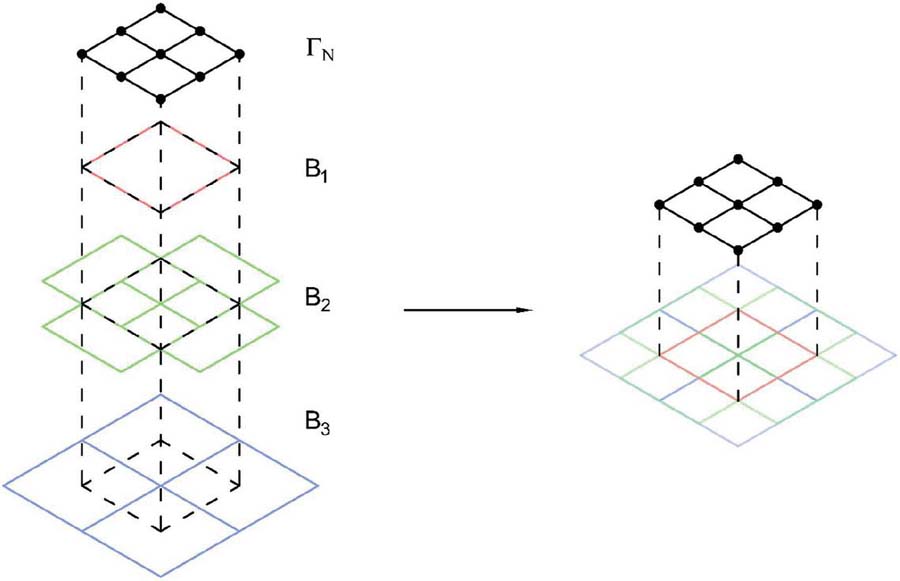
Let be discretised by linear hexahedral elements, such that is composed of edge-faces and their corresponding nodes. It is again assumed that a random field X has been generated over such that it holds values at the nodes of , and represents a property of the domain. The same process can be carried out in 3-D as in 2-D, where the blocks are now considered to be surfaces over which the flux will be distributed. The simplest case in this setting – other than a single element or pseudo 1-D configuration – is shown in Figure 3, where comprises 4 edge-faces and 9 nodes.
Figure 3 Schematic to show the block structure, where B1, B2, and B3 combine to form the block layer over which the flux is redistributed.
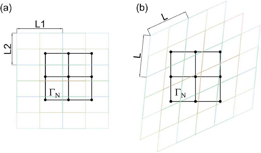
In the given figure, the blocks are assumed to be square and align neatly with the mesh. As in 2-D, the alignment of the blocks with the mesh is not strictly necessary, and is done so here for clarity of illustration. Similarly, the assumption of perfectly square blocks does not need to be enforced. It could be the case that the blocks are longer in one direction that the other, or that not all corner angles within the block are 90 as for a rhombus (see Figure 4(a) and 4(b) respectively).
Figure 4 Schematic of irregular block configurations where: (a) the blocks are longer on one side L1 L2, and (b) they blocks take the form of a rhombus.
The advantage of having irregular block configurations is the ability to represent anisotropic local effects due to neighbouring regions. In certain physical systems, it may be that an applied flux at a given position should see greater locally affects in one direction tangential to the surface than another. In this instance, having a larger block length in this direction would allow this greater region of influence to be accounted for. Furthermore, the main constraints are that the blocks should be able to be layered such that they can overlap at the midpoint of neighbouring blocks, as in Figure 3, and if irregular blocks are employed, the opposing angles of a block should be equal such that a rhombus is formed. It is noted that this study did not investigate further the use of irregular block formations.
In 3-D, the composition of blocks for a given node is less straight forward. The layers B, B, and B in Figures 3 and 6 are for illustration, and the composition of the blocks is not necessarily always split into a given number of layers. Instead, we define the scaled flux at the -th node as
| (22) |
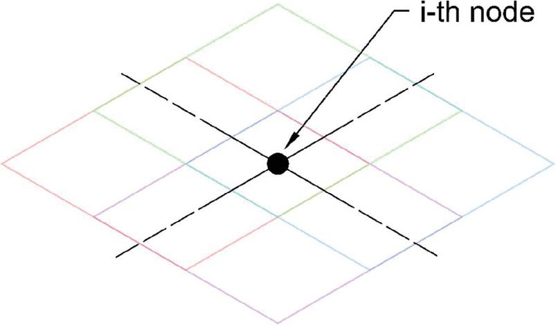
where is the set of all blocks containing the -th node, and is the pyramid shape function over the B-th block in . In this overlapping convention, the -th node will be contained within 4 blocks, as see in Figure 5.
Figure 5 Schematic of the block contribution for the -th node, where 4 blocks are used to scale the given flux value .
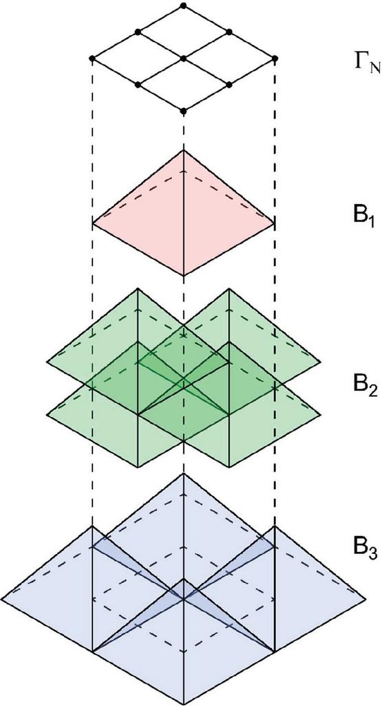
By aligning the blocks in this manner, the pyramid shape functions – which are nothing more than the product of two perpendicular hat shape functions aligned with each axis of the block surface – enforce a partition of unity for each position of the domain. This is seen in Figure 6, where the blocks and corresponding shape functions are grouped by patterns of alignment over . The implementation algorithm 1 is given below, where the same approach is taken in 2-D by replacing the expression for with Equation (21).
Figure 6 Schematic of the combination of shape functions from layers B, B, and B over .
As will be shown in the following section, the flexibility of the approach allows the applied flux field to be neatly coupled with the material response, such that it can vary with time. When conducting a time-dependent analysis, X will remain unchanged, suggesting that the flux applied to the surface will be distributed scaled and applied with the same variation throughout the analysis.
The alternative is to base the scaling of the boundary condition on a property that is changing in time as the condition is applied. If – as is seen in the later sections – , where is the primary variable being simulated in , then the flux will be scaled depending on the response of the medium. A schematic of this is seen in Figure 7.
Figure 7 Schematic to show the effects of a time-dependent flux surface for a diffusive process, where the quantity that the flux is scaled by evolves in time.
Consider the case where , and a given block contains a collection of nodes. Illustrated in Figure 7 are two of said nodes whose nodal values are denoted as and , where and are much larger relative to the other nodes of the given block. Based on the scaling framework, more flux should be applied to and , with receiving a larger amount, as is shown by the surface. This will lead to high injections of flux into the medium at these position as opposed to the rest contained in the block. If it is assumed that a diffusive process is being simulated, then as time advances, the mass injected into the system at and will begin to diffuse to the surrounding nodes, meaning less flux is distributed to and as they are smaller relative to the surrounding nodes. This leads to the variations in the flux at the surface beginning to diffuse, and a trend towards a more uniform flux application across the surface. Clearly, the behaviour here is dependent on the nature of the transient evolution of the solution, as well as the chosen property that the flux surface depends upon. In the previous section, it could have been assumed that X represented scalar values of material properties, such as Young’s modulus or permeability, leading to a non-evolving flux application.
4 Application: Moisture Transfer in Spatially Varying Soils
Here, the proposed heterogeneous boundary condition is applied to simulate moisture transfer in unsaturated soil, in order to examine the effect that the scaled flux surface has on the patterns of infiltration.
Random fields are utilised to introduce heterogeneity into the domain, namely through spatially varying the saturated conductivity , and van Genuchten parameters and . These will directly influence the Darcian type flow that is present in the medium by varying the constitutive components of the model. The soil water retention curve is calculated using the well-known van Genuchten model
| (23) |
and the standard van Genuchten – Mualem model is used to represent the relative permeability
| (24) |
where is the degree of saturation, and . Darcy’s law depends on the unsaturated hydraulic conductivity , and is calculated using Equation (24) and as
| (25) |
It can be seen that these material properties will vary spatially due to the variation in the chosen parameters stated above, as they either depend explicitly or implicitly on spatially varying parameters. For further details on the model and the effects of spatial variability on flow in soils, see Ricketts et al. (2023a).
The material properties, given in Table 1, of the simulated soil are based on those given by Wang et al. (2003) for a sandy loam
| Saturated Conductivity, m/s | , Pa | – | Porosity – | (Vertical) m | Density of Water kg/m | |
| Mean Value | 7.1 10 | 0.0008 | 1.8 | 0.35 | 0.3 | 1000 |
| Standard Deviation | 2.3 10 | 0.00015 | 0.01 | – | – | – |
The domain is a 1 m 1 m 1 m cube discretised by regular hexahedral elements, composed of 9261 nodes and 8000 elements (with appropriate convergence checks undertaken). The applied flux to be scaled is given as 1.5 cm h applied for a duration of 7 hours, which may be thought of as a rainfall condition upon the soils surface. After the first 7 hours, the analysis is run for a further 22 hours to simulate moisture to redistribution within the domain. Here, the block length is chosen to be equal to , the correlation length of the soil parameters. Generally, the local effects at a given point in – when heterogeneity is present – should be relative to as this is nothing more than the distance over which values are correlated. Namely, points outside of this region of influence should have little to no effect on the response at its centre. This type of continuous representation makes the choice of the block length relatively straightforward. To enable a sufficiently smooth field representation, 5 elements are usually taken within each correlation length, and as this is our block length, this satisfies the condition of having a sufficient number of nodes per block. Generally, the choice of block length must relate to the region of influence that a given point in the domain has on its neighbours, and contain at least 2 nodes.
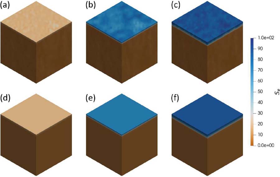
Figure 8 Short-term wetting response when applying a homogenous Neumann boundary condition, where (a–c) and (d–f) depict a heterogeneous and homogeneous domain respectively at: (a), (d) 10 minutes, (b), (e) 26 minutes, and (c), (f) 60 minutes.
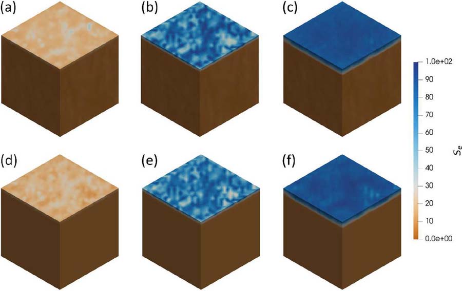
Figure 9 Short-term wetting response when applying a heterogeneous Neumann boundary condition scaled based on , where (a–c) and (d–f) depict a heterogeneous and homogeneous domain respectively at: (a), (d) 10 minutes, (b), (e) 26 minutes, and (c), (f) 60 minutes.
To clearly observe the influence of heterogeneous boundary conditions on the resulting infiltration patterns, 6 configurations of varied domain type and boundary condition were analysed. In all the presented cases, the variability over is kept constant to allow comparison of response to be made. There are two cases for , namely when the material properties in the soil body vary spatially, and when they are homogeneous, the latter being denoted by . This is done such that the effects of the differing boundary conditions on flow can be observed clearly, decoupling the influence of heterogeneity present in the medium. The flux scaling scenarios are a homogenously applied flux surface, scaling based on the saturated conductivity , and scaling based on unsaturated conductivity . The main difference here is that , and so the flux surface will evolve in time based on the evolution of liquid phase throughout the domain.
Figures 8, 9 and 10 show the progression of a wetting front over a given time frame, where the main difference is the boundary condition being applied. Figures, (a–c) and (d–f) represent solutions over and respectively, where the times are 10 minutes for (a) and (d), 26 minutes for (b) and (e), and 60 minutes for (c) and (f). Figure 8 shows the front after applying a homogeneous boundary condition, Figure 9 shows the front after scaling the flux based on , and finally Figure 10 shows the resulting wetting front after scaling the flux based on .
Figure 10 Short-term wetting response when applying a heterogeneous Neumann boundary condition scaled based on , where (a–c) and (d–f) depict a heterogeneous and homogeneous domain respectively at: (a), (d) 10 minutes, (b), (e) 26 minutes, and (c), (f) 60 minutes.
It is clear that the response at the boundary is quite different in all cases based on the evolution of the degree of saturation (DOS) at . As expected, Figure 8 (d-f) gives the expected response when applying uniform boundary conditions to a homogenous domain, such that the front is stable and advances with time through the medium. In contrast, when the domain is heterogeneous, the front builds up more in regions where the conductivity is lower and diffuses quickly through high regions of conductivity.
A more marked difference from the homogeneous response is observed when the applied flux is varied based on . As is expected, the regions where is larger receive more water compared with low conductivity zones, and is seen in Figure 9(a). As time advances, the applied flux field remains constant – as is unchanging – such that in (b) and (c), the areas where the moisture is generally highest relate to those in (a) that have a higher DOS. Mass is continually forced into these areas over the time that the flux is applied, leading to a pattern of infiltration based largely on . This is also true for (d–f). The main difference here when simulating over is that the front will diffuse uniformly in all directions for a given point in the domain. This leads to the less uniform distribution of moisture on the surface of (f) when compared against (c). The fluid is forced in larger quantities to the areas of high , but once this happens, the moisture present will diffuse uniformly due to the homogenous conductivity. In the case of (c), even though more mass is applied in the conductive regions, there is less build up here as the heterogeneity of the domain allows it to diffuse faster into the surrounding media.
Finally, Figure 10 shows the most distinct response for all (a–f) in the three figures considered. The response here, specifically in the initial stages of the analyses, can be thought of as the fluid following the paths of least resistance locally, entering into large pores, and reducing the available water for its neighbours. This is illustrated in (a) and (d) by the injection of flux in distinct location on . As this fluid begins to diffuse around these points, the conductivity in the plumed regions will rise, forcing the flux in the next time step to be spread more evenly across the plumes. Physically, this is a result of rising DOS and conductivity of the plumed areas, where water would be able to enter much more easily. From (b) to (c), and (e) to (f), these plumes grow, until eventually the applied flux is transformed from a surface containing sharp peaks at very localised positions, to a much more uniform application due to the growing level of saturation across .
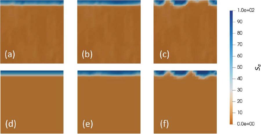
To further highlight the various forms of wetting fronts seen when applying the flux, slices were taken in each of the 6 cases after 1 hour. These are seen in Figure 11 where the applied boundary conditions are: (a,d) homogeneous Neumann, (b,e) heterogeneous Neumann scaled based on , and (c,f) heterogeneous Neumann scaled based on (where (a–c) and (d–f) are solutions from and respectively). It is clear than for (a) through (c) and (d) through (f), that the invading fluid phase becomes more distinct. It is also clear that, whilst the heterogeneity present in the domain is having an effect on the front, the influence of the heterogeneous boundary conditions further adds to this change in response.
Figure 11 Vertical profiles of infiltration at 1 hour, where the applied boundary conditions are: (a,d) homogeneous Neumann, (b,e) heterogeneous Neumann scaled based on , and (c,f) heterogeneous Neumann scaled based on (where (a–c) and (d–f) are heterogeneous and homogeneous domains respectively).
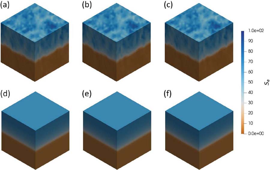
The cases that have been considered here have all been in a relatively short time frame when compared with the total simulation time. Figure 12 shows the fronts after the final simulation time of 29 hours.
Figure 12 Final wetting fronts at 29 hours where the applied boundary conditions are: (a,d) homogeneous Neumann, (b,e) heterogeneous Neumann scaled based on , and (c,f) heterogeneous Neumann scaled based on (where (a–c) and (d–f) are heterogeneous and homogeneous domains respectively).
It is clear that after the full simulation time, the fluid phase has had time to diffuse into the domain laterally and vertically, forming wetting fronts that are similar for each boundary condition considered. The difference here is only seen between (a–c) and (d–f) due to the level of heterogeneity present. As the analysis advances and the boundary condition is turned off, the flow through the medium is governed by the properties of the soil body, and as (a–c) and (d–f) are identical in this manner, it is reasonable that their responses should converge.
In all cases, the response across the surface is largely dependent on the observation time frame. The constitutive relations in the model ensure that as the DOS rises, the values of across will converge to , meaning that if enough mass is applied over a given length of time, the flux surfaces will converge. If the flux was continued to be applied after reaching saturated conditions, the flux field being applied would be the same when scaled based on or . Whilst this is true for the physical system considered in this study, there may be instances where material relations are employed that do not follow this convergent behaviour, but this has not been addressed.
5 Concluding Remarks
The conclusions of this study are given as follows:
• The simulated response of many physical systems is strongly dependent on the way in which boundary conditions are applied. This depends on the type of system, as well as the time-scale over which the processes are being represented. In Section 4, the differences between the responses of analyses with different boundary conditions reduce with time over the period of the analysis, with the differences becoming negligible with increasing time. For other systems, materials, or simulation configurations, this may not be the case, and applying boundary conditions in this manner can lead to a more natural application of mass based on the physical properties of the medium.
• For soils, the inclusion of the scaled condition leads to a more natural response of infiltration, where the choice of dependence on a constant parameter such as or an evolving parameter such as depends on the soil being simulated.
• A key benefit of the method is that it is independent of the discretisation and order of interpolation employed. As the blocks are simply “macro-elements”, they can be position across a domain surface in many configurations regardless of the numerical techniques used in the solution process. This makes its adoption into existing codes less intrusive, as it can be carried out as a self-contained process in each time step.
• The ability to implement irregular blocks would allow for anisotropy of local effects to be accounted for. For example, if the boundary condition is not applied normal to the surface, then there could be greater local influence in a given direction, for example runoff on a slope. By scaling the blocks, this local phenomenon could be represented. Another assumption is the overlapping principle that should be maintained through the block layers. This specific configuration is chosen such that a partition of unity can be achieved with linear shape functions; however, this does not imply that other overlapping configurations with different shape functions would not lead to alterative or similar responses. With the choice of appropriate shape functions and subsequent overlapping to form a partition of unity, this could lead to more intricate local effects being accounted for.
• It is clear that the response at the surface is strongly influenced by implementing such a method. This can be tailored to experimental observations by careful choice of the variable that the scaled flux field is dependent on. Furthermore, the method shows great flexibility in representing alternate responses at the surface of a given medium when simulating complex systems.
Acknowledgements
The authors would like to acknowledge the School of Engineering at Cardiff University and LUSAS for collectively funding this project.
References
Bolin, D. and Kirchner, K. 2020. The Rational SPDE Approach for Gaussian Random Fields With General Smoothness. Journal of Computational and Graphical Statistics 29(2), pp. 274–285. doi: \nolinkurl10.1080/10618600.2019.1665537.
Brune, P., Duan, J. and Schmalfuß, B. 2009. Random Dynamics of the Boussinesq System with Dynamical Boundary Conditions. Stochastic Analysis and Applications 27(5), pp. 1096–1116. doi: \nolinkurl10.1080/07362990902976546.
Cerrai, S. and Freidlin, M. 2011. Fast transport asymptotics for stochastic RDEs with boundary noise. The Annals of Probability 39(1). doi: \nolinkurl10.1214/10-AOP552.
Chitez, A.S. and Jefferson, A.D. 2015. Porosity development in a thermo-hygral finite element model for cementitious materials. Cement and Concrete Research 78, pp. 216–233. doi: \nolinkurl10.1016/j.cemconres.2015.07.010.
Cleall, P.J., Seetharam, S.C. and Thomas, H.R. 2007. Inclusion of Some Aspects of Chemical Behavior of Unsaturated Soil in Thermo/Hydro/Chemical/Mechanical Models. I: Model Development. Journal of Engineering Mechanics 133(3), pp. 338–347. Available at: https:/ascelibrary.org/doi/10.1061/\%28ASCE\%290733-9399\%282007\%29133\%3A3\%28338\%29.
Darcy, H. 1856. Les fontaines publiques de la vile de Dijon. Paris, Dalmont.
Fuglstad, G.-A., Lindgren, F., Simpson, D. and Rue, H. 2013. Exploring a New Class of Non-stationary Spatial Gaussian Random Fields with Varying Local Anisotropy.
Guo, J., Veran-Tissoires, S. and Quintard, M. 2016. Effective surface and boundary conditions for heterogeneous surfaces with mixed boundary conditions. Journal of Computational Physics 305, pp. 942–963. doi: 10.1016/j.jcp.2015.10.050.
Lasanen, S. 2002. Discretizations of Generalized Random Variables with Applications to Inverse Problems.
Lindgren, F., Rue, H. and Lindström, J. 2011. An explicit link between Gaussian fields and Gaussian Markov random fields: the stochastic partial differential equation approach.
Liu, W.F. and Leung, Y.F. 2018. Characterising three-dimensional anisotropic spatial correlation of soil properties through in situ test results. Géotechnique 68(9), pp. 805–819. doi: 10.1680/jgeot.16.P.336.
Mariano, A.J., Chin, T.M. and Özgökmen, T.M. 2003. Stochastic boundary conditions for coastal flow modeling. Geophysical Research Letters 30(9), p. 1457. Available at: http:/doi.wiley.com/10.1029/2003GL016972.
Mohammed, W.W. 2015. Amplitude equation for the stochastic reaction-diffusion equations with random Neumann boundary conditions. Mathematical Methods in the Applied Sciences 38(18), pp. 4867–4878. doi: 10.1002/mma.3402.
Nielsen, D.R., Th. Van Genuchten, M. and Biggar, J.W. 1986. Water flow and solute transport processes in the unsaturated zone. Water Resources Research 22(9S), pp. 89S-108S. doi: 10.1029/WR022i09Sp0089S.
Da Prato, G. and Zabczyk, J. 1993. Evolution equations with white-noise boundary conditions. Stochastics and Stochastic Reports 42(3–4), pp. 167–182. Available at: https:/www.tandfonline.com/doi/full/10.1080/17442509308833817.
Da Prato, G. and Zabczyk, J. 1996. Ergodicity for Infinite Dimensional Systems. Cambridge University Press. doi: 10.1017/CBO9780511662829.
Rasmussen, C.E. and Williams, C.K.I. 2005. Gaussian Processes for Machine Learning. The MIT Press. doi: 10.7551/mitpress/3206.001.0001.
Ricketts, E.J., Cleall, P.J., Jefferson, A., Kerfriden, P. and Lyons, P. 2023a. Representation of three-dimensional unsaturated flow in heterogeneous soil through tractable Gaussian random fields. Géotechnique, pp. 1–34. doi: 10.1680/jgeot.22.00316.
Ricketts, E.J., Cleall, P.J., Jefferson, T., Kerfriden, P. and Lyons, P. 2023b. Near-boundary error reduction with an optimized weighted Dirichlet–Neumann boundary condition for stochastic PDE-based Gaussian random field generators. Engineering with Computers. doi: 10.1007/s00366-023-01819-6.
Roininen, L., Huttunen, J.M.J. and Lasanen, S. 2014. Whittle-matérn priors for Bayesian statistical inversion with applications in electrical impedance tomography. Inverse Problems and Imaging 8(2), pp. 561–586. doi: 10.3934/ipi.2014.8.561.
Satish, M.G. and Zhu, J. 1992. Stochastic approach for groundwater flow in a semiconfined aquifer subject to random boundary conditions. Advances in Water Resources 15(6), pp. 329–339. doi: 10.1016/0309-1708(92)90001-I.
Shi, L., Yang, J., Cai, S. and Lin, L. 2008. Stochastic Analysis of Groundwater Flow Subject to Random Boundary Conditions. Journal of Hydrodynamics 20(5), pp. 553–560. doi: 10.1016/S1001-6058(08)60094-3.
Wang, W. and Duan, J. 2007. Homogenized Dynamics of Stochastic Partial Differential Equations with Dynamical Boundary Conditions. Communications in Mathematical Physics 275(1), pp. 163–186. doi: 10.1007/s00220-007-0301-8.
Wang, Z., Wu, L., Harter, T., Lu, J. and Jury, W.A. 2003. A field study of unstable preferential flow during soil water redistribution. Water Resources Research 39(4). Available at: http:/doi.wiley.com/10.1029/2001WR000903.
Xu, S. and Duan, J. 2011. A Taylor expansion approach for solving partial differential equations with random Neumann boundary conditions. Applied Mathematics and Computation 217(23), pp. 9532–9542. doi: 10.1016/j.amc.2011.03.137.
Zienkiewicz, O.C., Taylor, R.L. and Zhu, J.Z. 2013. The Finite Element Method: its Basis and Fundamentals. Elsevier. doi: 10.1016/C2009-0-24909-9.
Biographies

Evan John Ricketts Lecturer in numerical methods at the School of Engineering, Cardiff University. His research journey began with numerical investigations of unsaturated flow in heterogeneous soils. This has since evolved to include areas of geotechnical engineering, machine learning and generative AI, and materials research, such as the simulation of heterogeneous materials through Gaussian random fields, multi-scale simulations, and approaches to discrete random field generation.

Peter John Cleall Professor of Geo-environmental Engineering, School of Engineering, Cardiff University. His research activities initially focused on the area of coupled flow and deformation behaviour in soils and have developed to encompass a number of areas in the subject of geoenvironmental and geotechnical engineering including ground energy, thermal fluxes and inter-seasonal heat storage, in-situ resource recovery from geological repositories and behaviour of modified soils. Work in these areas, supported by RCUK and industrial funding has developed a number of specific analytical and numerical models alongside an improved understanding of fundamental processes.

Anthony Jefferson studied at Swansea and Cardiff universities and obtained PhD from Cardiff. He spent 10 years with a firm of consulting engineers before joining Cardiff University in 1994. He undertakes research on the computational modelling of cementitious and self-healing materials, and the development of new construction material systems. His chair is sponsored by the software company LUSAS.

Pierre Kerfriden their scientific interests lie in the field of advanced numerical methods for the simulation of complex physical phenomena described by partial differential equations. Applications range from the prediction of fracture in composite materials to the control of micromanufacturing processes. Their research focuses on the development of multiscale numerical solvers and automated, data-driven complexity reduction methods.

Paul Lyons is the founder and managing director of the international engineering software company LUSAS. He founded LUSAS in 1982 and has led the company throughout its history. He has a PhD from Imperial College and has been a visiting professor at Imperial College and Cardiff University.
European Journal of Computational Mechanics, Vol. 33_3, 199–226.
doi: 10.13052/ejcm2642-2085.3331
© 2024 River Publishers


