Estimation of Passive Drag in Swimming via Experimental and Computational Means
Alex Haskins1,*, Carla McCabe2, Ryan Keating2, Alex Lennon1 and Dominic Chandar1
1School of Mechanical and Aerospace Engineering, Queen’s University Belfast, Belfast, BT9 5AH, UK
2School of Sport, Ulster University, Belfast, BT15 1AP, UK
E-mail: ahaskins02@qub.ac.uk; c.mccabe@ulster.ac.uk; r.keating@ulster.ac.uk; a.lennon@qub.ac.uk; d.chandar@qub.ac.uk
*Corresponding Author
Received 29 November 2023; Accepted 04 June 2024
Abstract
Discussed is a comparison of computational and experimental evaluations of passive drag during human swimming. Experimentally, ten trials were conducted per athlete at five chosen velocities, using a commercial resistance trainer to record the tension force in a rope during a streamline position tow test. The resistive force recorded was assumed equal to the passive drag force and an average value of passive drag was found across each tow test. Mean passive drag values measured during the tow test were agreed well with existing experimental data across the range of velocities used, varying between 20 N at 1 ms up to 100 N at 2 ms. Computationally, using the immersed boundary method in OpenFOAM, basic geometry validation cases and streamline passive drag cases were simulated. Validation cases were completed on 2D cylinders and 3D spheres with the drag coefficient found at low and high Reynolds numbers, using the simpleFoam solver within OpenFOAM. Results tended to be slightly over predictive when compared with existing simulation and experimental data in literature. The accuracy of results could potentially be improved using a finer mesh and better quality geometries. The passive drag was also computed using OpenFOAM over a range of velocities, similar to the experiments, varying from 30 N at 1 ms to 120 N at 2 ms. Drag forces computed using simpleFoam were over predictive when compared to existing literature and the completed experiments, likely due to the inaccuracy of the geometry used in the simulations. When results were compared to existing literature for swimmers not in a perfect streamline position, more similar to the geometry used in this study, results were in better agreement. The accuracy of the results could be improved using a better quality geometry in the correct position.
Keywords: Immersed boundary method (IBM), passive drag, OpenFOAM, validation.
Introduction
Passive drag is the resistance generated by a swimmer’s body whilst the swimmer moves through the water in a fixed position [1, 2] and is typically composed of frictional, pressure, and wave drag. Passive drag acts on the swimmer during the glide phases of the stroke, such as when streamlining off the wall or following a dive-entry [3]. The streamline position is typically the phase of a race with the highest velocity, due to the explosive nature of a diving start or wall push-off. Accounting for passive drag could allow for better understanding of how to maximise velocity during these streamline phases. Passive drag is typically investigated via experimental and computational methodologies, as outlined below.
Passive drag experiments are common in literature, with the earliest examples involving swimmers being towed aft of a rowboat, with the resistive force measured using a dynamometer and assumed equal to the passive drag force [4]. Towing is one of the more common methods for finding a passive drag value, with typical tow rigs making use of either electric motors or a weight and pulley system [5, 6]. The swimmer is attached to a rope under tension before being towed towards the motor or pulley whilst in a streamline position. Typically, the athlete is towed at a constant velocity, with a dynamometer measuring a resistive force value. The experiment is typically repeated at a number of different velocities in order to investigate the drag-velocity relationship for an individual athlete [7]. The towing method is accepted as one of the more accurate estimation methods of passive drag and as such there is little variation to the method with time [7].
The flume method is another experimental method of determining passive drag, acting like an aquatic treadmill, with precisely controlled water inlet velocity [8, 9]. Similar to the towing method, the swimmer is attached to a length of rope in a streamlined position, with the rope attached to a dynamometer. Fans controlling the water velocity are then turned on and create moving water around the stationary swimmer. The dynamometer then records the force at which the swimmer is pushed away by the moving water, which is assumed to be equivalent to the passive drag of a swimmer. Passive drag results found via the flume method tend to agree well with the towing method, with five separate studies finding passive drag values of approximately 110 N, at a flow velocity of 2 ms using both flume and towing methods [10]. Although the flume method does provide an accurate measurement of passive drag, there are differences between free swimming and flume swimming, such as wall impact on flows and velocity variations, which will lead to inaccuracies within the flume method [7, 11, 12].
A further method of predicting passive drag is via the gliding decay method, first developed by Bilo and Nachtingall [13] by looking at birds and aquatic animals, with the first human passive drag trial completed by Kjendlie and Stallman [14]. A typical testing protocol involves a swimmer submerging and pushing off the wall in a streamlined position, causing an acceleration, followed by a deceleration due to the resistive forces of the water acting on the streamlined body. Resistive forces can be estimated by finding the instantaneous deceleration via cable accelerometers, underwater video analysis, and body mass of the swimmer [14, 15]. An extra water mass is moved together, with the swimmer and their body mass, which must be considered as part of the inertia. This is difficult to calculate due to the dependence on several factors such as area of impact and hydrodynamic coefficient. It is common in literature for this added mass to be ignored [15]. This method of determining passive drag is cheap, with results comparable to flume and towing methods, although drag values tend to be consistently higher in past studies [7]. Negatives of the method include difficulties in maintaining depth, with athletes often rising to the surface, and the added complexity of added mass [7, 16].
Passive drag can also be investigated computationally via the use of computational fluid dynamics (CFD). Passive drag simulations have been run in both 2D and 3D, for steady state and unsteady flow conditions [17]. Typical methods will make use of a body-fitted grid with the region around the geometry refined to the required level, trying to capture the flow as accurately as possible. Many simulations to date have successfully implemented a turbulence model, with the k- model very common. Accuracy of these simulations can be greatly impacted by the accuracy of the geometry on which simulation work is being carried out [7]. Accuracy is also limited by the refinement level of the mesh used to capture the fluid flow, with refinement limited by the available computational hardware. One method to avoid body fitted meshes around complex shapes is to employ the immersed boundary method (IBM), as explained in more detail in the theory section below. There is an example of an IBM used in order to model the flow around a swimmer during underwater butterfly kick, although no drag force calculation was completed. The IBM method used was a ghost cell method using a finite difference approximation and LES turbulence modelling in order to predict flow features around the swimmer [18, 19].
Several CFD simulations have demonstrated accurate estimation of drag when compared to towing and flume methods, but are very reliant on detailed reproduction of the geometry and motion of the swimmer, both of which present considerable challenges for conventional body-fitted CFD approaches [7].
This study aimed to investigate the accuracy of single-phase CFD simulations for predicting the passive drag of a swimmer, using the immersed boundary method. Suitability of the method was assessed by comparing predicted drag forces with existing simulation literature and with a series of experimental passive drag tow tests.
Theory and Governing Equations
The incompressible turbulent flows that are being considered in the following simulations are governed by the continuity and momentum equations, included below [20]:
| (1) | |
| (2) |
where u is the velocity vector, p is the pressure, is the kinematic viscosity, and S is a general source term for additional forcing terms, which in this case is not required. The solutions to the governing equations are approximated using the finite-volume method (FVM). In the FVM, the computational domain is divided into finite volumes and the governing equations are discretised using appropriate numerical schemes [20].
Foam-extend [21], a fork of OpenFOAM, was used as a solver for all computations. Since the focus is on single-phase passive drag validation, only single-phase steady-state calculations were conducted using the simpleFoam solver within foam-extend. The simpleFoam solver uses the SIMPLE algorithm [22] to resolve the pressure-velocity coupling for incompressible flows.
Turbulence
Due to the high Reynolds number of the flow being considered, approximately 4 million, turbulence models must be introduced to model near wall physics. During simulations the Reynolds Averaged Navier-Stokes (RANS) equations are used, instead of the Navier-Stokes equations. During the Reynolds decomposition, the velocity is divided into a mean component, , and a fluctuating component, . Following the decomposition for the continuity and momentum equations, time averaging the equations results in the following RANS equations [20]:
| (3) | |
| (4) | |
| (5) | |
| (6) |
where U is the mean velocity vector, u is the fluctuating velocity vector, and are mean velocity components and , and are fluctuating velocity components. During the time averaging of the convection term, a new term with fluctuating velocities appears, known as the Reynolds stress term. Turbulence models are used to close the RANS equations, in these cases the two-equation k- and k- models are used [20].
The Boussinesq hypothesis states the Reynolds Stresses are proportional to the mean deformation rates and can be described for incompressible flows as follows [20]:
| (7) |
where is the eddy viscosity and is the turbulent kinetic energy per unit mass:
| (8) |
In the k- and k- models’ transport equations, the turbulent kinetic energy, k, the viscous dissipation rate, , and the rate of specific dissipation, , are used to predict the kinetic energy, turbulent viscosity, and Reynolds stresses [20].
k- Turbulence Model
The turbulent kinetic energy, , and the viscous dissipation rate, , are used to define the velocity, , and length, , scales of the large-scale turbulence as below [20, 23]:
| (9) | |
| (10) |
The eddy viscosity can then be described using and , with the help of the velocity and length scales, as follows:
| (11) |
where is a dimensionless constant. The standard k- model, developed by Launder and Spalding, used within OpenFoam uses simplified transport equations as below [20, 24]:
| (12) | ||
| (13) |
SST k- Turbulence Model
The SST k- model, developed by Menter [25], is a two equation eddy-viscosity model making use of the shear stress transport (SST) formulation. The model is based on the following formulation:
| (14) | ||
| (15) |
where is a production limiter and is a blending function, as described by Dohler [14]. In the freestream of the flow, the blending function is set equal to 0, meaning the k- is used. is set to equal 1 in the boundary layer, meaning the Wilcox k- model is used. From Menter et al, the coefficients in Equations (14) and (15) are a combination of the k- and k- models as follows [20, 25].
Wall Models
Wall models are used to model near-wall physics so as to allow a coarser mesh to be used near the wall region. The refinement level of the mesh is dictated by the y+ value, defined as the dimensionless quantity for the distance from the wall to the centre of the first grid cell. The approximate y+ value when using turbulence models should be 30 y+ 300. The immersed boundary method within Foam-Extend-5.0 has its own set of k- wall models, for each variable. In this case, the cells were refined such that the non-dimensional cell height is approximately equal to 30, although having a y+ value of exactly 30 can prove difficult [20].
The Immersed Boundary Method (IBM)
The immersed boundary method, developed by Peskin [26], was designed in order to remove the need for a body fitted grid. The method typically accounts for solid boundaries in the discretised domain by altering the governing equations by a source term. However, the IBM in foam-extend is based on a more conservative approach that uses a cut-cell method rather than adding a source term to account for the presence of a physical boundary. The cut-cell method cuts intersected cells at the location of the immersed boundary, conserving mass and momentum near the boundary. The cells are reshaped into trapezoids, with living cells (active) added to the fluid cells and dead cells added to the body cells. For the discretisation, the mass, momentum, convective and diffusive fluxes, and the pressure gradients must be evaluated on all cell faces [20].
The cut-cell method in foam-extend-5.0 goes by the name – Immersed Boundary Surface Method (IBS). Within this method three cell types exist: solid (dead), intersected, and fluid (live) cells, with all intersected cells identified as immersed boundary cells, as shown in Figure 1 [20]:
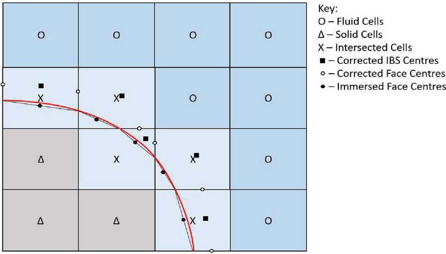
Figure 1 Diagram of the immersed boundary cut cell method implemented within Foam-Extend-5.0.
The intersected cells are cut by the immersed boundary, with a linear cut between intersection points of each intersected cell. The cells are then divided into live and dead volumes and faces. The new fluid volumes become a live cell with a new cell centre and volume calculated, as well as new face area, face centre, and face area vector for the cut faces and new immersed boundary face. All dead cells are removed from the discretisation matrix, with the new geometry data of the new live part of the cut cells replacing old cut cell data. This means the immersed boundary can be added as a body fitted boundary condition on the fluid cells and the conventional FVM can be employed [20, 27].
Closed cells must be ensured after the cutting process via the Marooney Manoeuvre. For normal cells the summation over all faces should be zero [20]:
| (16) |
For open cell interfaces, the Marooney Manoeuvre is implemented, with old surface face areas, , corrected by a face correction, . The corrected immersed boundary face area, , can then be added to the summation as follows [20]:
| (17) |
The IBM allows meshing of moving body problems to be simplified as a new body fitted mesh is not required for each geometry position of the moving body, reducing computational requirements, although the cases discussed in this study are not moving body problems [20].
Drag Force
The final passive drag forces acting on the body are a combination of the normal pressure force and the tangential viscous forces as shown below [28]:
| (18) |
Where i is the identified cell, is the passive drag, is the density of the fluid, is the face area vector, is the pressure, is the dynamic viscosity, and is the deviatoric stress tensor.
Experimental Methodology
Participants
Ten athletes, evenly split as 5 males and 5 females, who train in the top squads in Lisburn City Swimming Club (Northern Ireland, UK), participated in the study. All athletes involved in the testing were required to be at least 16 years old (anthropometric details in Table 1).
Table 1 Anthropometric data of the athletes
| Height (m) | 1.72 0.18 |
| Chest Depth (m) | 0.22 0.03 |
| Shoulder Width (m) | 0.39 0.06 |
| Mass (Kg) (8 athletes only) | 67.81 18.79 |
Ethics Approval and Consent to Participate
This study was approved by the local Queen’s University Belfast ethics committee, namely the Engineering and Physical Sciences Faculty Research Ethics Committee, and was performed in accordance with the guidelines and regulations of the Declaration of Helsinki. All participants were provided with verbal and written explanations of the purpose, procedure and risks related to the study and provided written consent. Informed consent was obtained from all participants of the study.
Equipment
The equipment used to tow the athletes was a 1080 Sprint [29] (1080 Motion, AB, Lindingo, Sweden) robotic resistance device, able to record resistive force readings at a sampling frequency of 333 Hz for a constant towing velocity that is pre-set into the device by the operator. The 1080 Sprint records the tension force in the rope, distance, and velocity of the athlete across the towing distance, at each timestep.
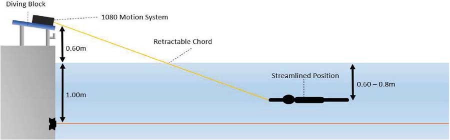
Figure 2 Diagram of the passive drag tow experiment.
Experimental Procedure
Figure 2 displays the equipment set up for the passive drag tows. The 1080 Sprint was mounted on a diving block at approximately 0.72 m above the surface of the water. A red rope attached at both ends of a 25 m pool was used to identify a depth of 1 m below the water’s surface, acting as a depth reference to aid the athletes’ ability to maintain constant water depth. Anthropomorphic data was collected after the experimental towing had been completed.
The athletes were instructed to enter the water and would begin each trial in the water facing the 1080 Sprint at a distance of 25 m from the equipment, with the towing velocity pre-set into the 1080 sprint. The athletes were attached to the 1080 Sprint via an additional piece of rope attached around their hands that was then harnessed to the equipment’s tether. The athletes were instructed that they would be towed in a streamline position, with arms stretched out in front. The streamline position of the athlete is shown by the geometry in Figure 3, with arms outstretched, one hand on top of the other and feet pointed. Ensuring position uniformity across athletes is difficult, but the standard of experimental participants is sufficient such that variability in streamline position across the trial will be a minimum. Differences in position are likely to be anthropomorphic.
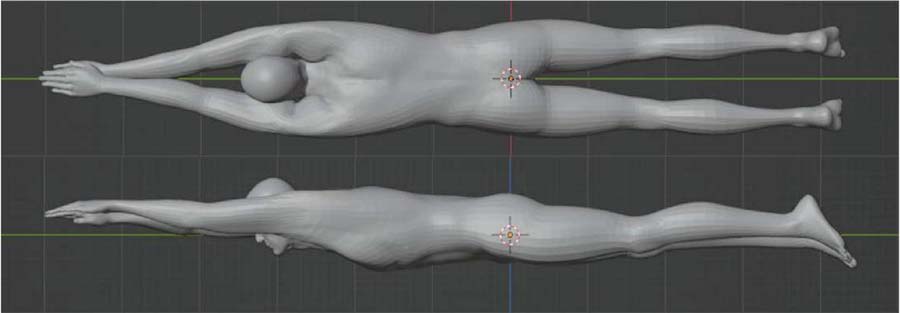
Figure 3 Diagram of approx. streamline position used by the athletes [30].
As the towing began, the athletes felt a slight tugging on the shoulders, indicating the tow had commenced. As the tow commenced, the athletes were instructed to submerge to a depth of 1m as quickly as possible, using the guide line as a depth guide, whilst maintaining a streamline position. The athletes were towed a distance of approximately 20 m whilst underwater in a streamline position. The athletes repeated the tow at each velocity twice. There were five predetermined velocities as follows: 1.00 ms, 1.25 ms, 1.50 ms, 1.75 ms and 2.00 ms. By the end of the full trial, each athlete had performed ten passive drag tows across the five velocities.
Post-Processing
During the experiments, 20 trials were completed for each of the five velocities. In order to select the trial results for post processing, the validity of each trial was checked using graphs of force against distance. Typical graphs tend to have an oscillatory motion, and one such trial is shown in Figure 4.
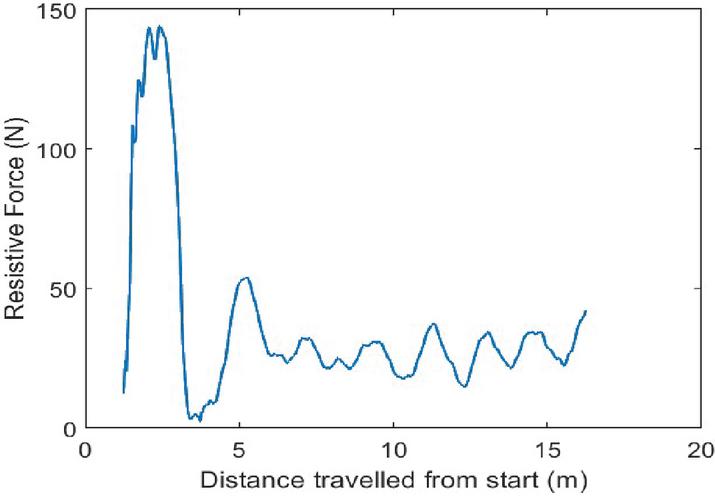
Figure 4 Raw data from one trial in the passive drag towing experiment.
For each completed tow, the Matlab [31] function findpeaks was used to identify the peak values of each oscillation. A minimum peak value constraint was added to ensure no artificially low peaks were identified and mistaken for the maximum resolved tension force values produced in the stroke cycle. This minimum peak value was set equal to the average value of the full passive drag tow. A boxplot of the peak values was then plotted in Matlab. Any peak values that lay outside the upper and lower limits of the boxplot were used to exclude the associated oscillation from the results. The first 5 m of the trial were discounted in each case as to allow the athlete time to reach both the required depth and an equilibrium, allowing the oscillation amplitude to reduce significantly. Due to the relatively short distance over which to collect data (15 m), data collected up until the finish of each tow has been used in the averaging process, as opposed to discounting the end of the data set. The remaining passive drag force data recorded by the 1080 Sprint was resolved to its horizontal component, based on the angle of elevation above the water as shown in Equation 19, before being averaged across the remaining passive drag data of the trial. The angle of elevation varied across the tow, based on the distance of the athlete from the equipment.
| (19) |
refers to the horizontal component of the raw tension force in the rope collected by 1080 Sprint, respectively (), when the rope is at an angle. The angle is the angle between the rope and the water of the 1080 Sprint. Gonjo and Olstad used a similar equation in their prediction of active drag to account for the impact of the angle of the rope caused by the height of their equipment [32].
Of the 20 trials for each velocity, two trials at each velocity have been discarded due to difficulty in processing results, leaving 18 full trials at each velocity for post processing. Of the 18 remaining full trials, 9 have the biological sex male and 9 have the biological sex female.
Statistical Analysis
Statistical analysis of measured towing forces was performed using the R Statistical Programming Language [33] and some additional packages. Specifically, data manipulation and exploratory analysis was performed using the ‘tidyverse’ ecosystem [34, 35] and ‘GGally’ [36] packages, and analysis of variance (ANOVA) was performed with the aid of the ‘rstatix’ package [37]. A mixed-design ANOVA (in which athlete sex was treated as a between-subjects factor and velocity was treated as a within-subjects factor, due to the repeated measurement of athletes across and within velocities) was used to investigate the contribution of athlete’s velocity and sex to measured drag force. Post-hoc contrasts were performed at each towing velocity, using multiple pairwise comparisons with Bonferroni adjustment, to investigate if there were any differences in mean drag force between males and females at each velocity. Assumptions of normality, homogeneous variance, and sphericity for the ANOVA were checked using common tests available in the ‘rstatix’ package. Mixed-effects regression analysis was performed using the ‘lme4’ package [38, 39] to investigate the ability of towing velocity and athlete-specific surface area to fit the measured drag force and to estimate drag coefficients for each sex. Mixed-effects regression differs from conventional multiple regression in that it allows separate assessment of factors that are hypothesised to directly affect mean response (fixed effects) and factors that contribute only to variance (random effects). To account for repeated measurements (due to each athlete being towed multiple times across different velocities and within each velocity) and other potential athlete-specific effects not captured by the anthropometric measurements, pseudonymised athlete ID was treated as a random effect for the mixed-effects analysis performed in this study. Visual inspection of residuals was used to check conformity with model assumptions.
Computational Procedure
Primitive Geometry Validation Cases
Firstly, validation was undertaken using geometric primitives. A 2D cylinder and a 3D sphere (Figure 5) were designed within Blender [40], before being imported into OpenFOAM [21]. Blender is an open source animation software capable of both geometric design and animation.
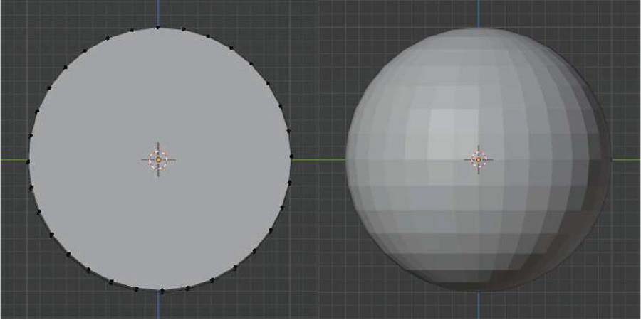
Figure 5 Blender geometries of a) 2D cylinder b) 3D sphere.
The 2D and 3D case setup was similar, with the 2D case slightly more involved. The first step was to create a Cartesian mesh using the blockMesh utility within OpeFOAM. A base grid size of 60x40 cells was employed for the 2D cases and a grid of 60x40x40 cells was used in the 3D cases. Following blockMesh, another utility called snappyHexMesh was used to refine the region around the geometry. Three mesh refinements were used for each of the 2D and 3D cases, namely a coarse, medium, and fine mesh. Due to the computational limits on the local supercomputer cluster, a fourth finer mesh dramatically increased the case set-up time and has not been completed.
Following mesh refinement using snappyHexMesh, extrudeMesh and autoPatch were used in the 2D case set-up to extrude the mesh from an existing patch and divide the external faces into patches based on a feature angle respectively. The feature angle, the angle above which a surface is not extruded, was 89 degrees in this case. The 2D mesh set-up was complete at this point. The number of cells in each of the 2D and 3D meshes are listed in Table 2.
Table 2 Number of cells in the 2D and 3D meshes
| Mesh Refinement Level | 2D Cell Count | 3D Cell Count |
| Coarse | 17766 | 96000 |
| Medium | 66864 | 1388788 |
| Fine | 1033380 | 10510719 |
Upon completion of mesh generation, the boundary and initial conditions were applied. Within the boundary folder of each case, an additional patch was added allowing for the immersed boundary condition to be applied. The new immersed boundary patch is treated like a wall with no internal flow permitted through the geometry.
There were two case conditions set for each level of mesh refinement for the 2D and 3D cases: a low Reynolds number of 20 and a high Reynolds number of either 10000 or 100000, depending on the use of the k- model or the k- model. In order to account for the change in Reynolds number, the kinematic viscosity was set at 0.1 ms for a low Reynolds number and either 210 ms or 210 ms for high Reynolds number simulations. The inlet velocity was set at 1 ms in all cases, with the density remaining constant in the incompressible simulations. The cases were decomposed, if required, to allow for parallelisation of the problem into the core distribution summarized in Table 3.
Table 3 Number of cores used in the 2D and 3D cases
| Mesh Refinement Level | 2D Number of cores | 3D Number of cores |
| Coarse | 8 | 8 |
| Medium | 8 | 24 |
| Fine | 16 | 128 |
The steady-state solver uses the SIMPLE algorithm in order to solve the velocity and pressure terms of the Navier Stokes equations. All cases were set to run for 10000 iterations, with the U, and k tolerances set as 110 and the P tolerance set as 110. The iteration number was reached before tolerance in a number of cases and at this point the simulation was stopped.
Swimmer Passive Drag Cases
Figure 6 displays the geometry that was used during the passive drag simulations, purchased from codethislab [30]. The geometry in Figure 3 was unusable, although the geometry is more reflective of a true streamline position, due to a large number of intersection points being present, which could result in simulation divergence if cells are tagged incorrectly. The geometry was imported into Blender for reshaping and translation. Due to the number of nodes in the geometry, there were limitations on the ability to reshape and translate the geometry due to the time consuming nature of the node manipulation. Other limitations were due to specific areas of the shoulders beginning to move into the volume of the body, which would usually be prevented by human skin. This could potentially cause errors in the CFD due to an open geometry. As such, the approximate streamline position shown in Figure 6 was the best approximation possible for this particular geometry. The geometry was then imported into OpenFOAM (version Foam-Extend-5.0).
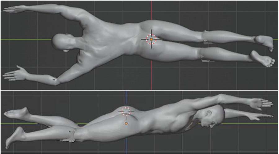
Figure 6 Streamline geometry for passive drag simulations.
Following a similar set-up to the validation cases, blockMesh was run to set-up the Cartesian mesh. A grid of 60x40x40 cells was used in the 3D passive drag cases. Following blockMesh, snappyHexMesh was used to refine the region around the geometry. Two regions were refined around the body: an inner region and an outer region, so as to maximise computational efficiency. The inner region was refined to a significantly finer mesh than the outer region, dictated by the refinement level selected. Three mesh refinements were used as a mesh convergence study; a fourth finer mesh resulted in the computational processes taking too long, likely due to hardware limitations. The cell counts for each refinement level are visible in Table 4.
Table 4 Number of cells in the swimmer geometry
| Mesh Refinement | Cell Count |
| Coarse | 1097084 |
| Medium | 7442290 |
| Fine | 57573014 |
Upon completion of mesh generation, the boundary and initial condition were applied. Unlike the validation geometry cases, the passive drag associated with changing, as opposed to constant, velocity was investigated. As such, the inlet velocity of the inlet flow was changed for the fine mesh simulations as follows according to the velocities listed in Table 5.
Table 5 Velocities used in CFD simulations
| Simulation Number | Simulation 1 | Simulation 2 | Simulation 3 | Simulation 4 | Simulation 5 |
| Velocity (ms) | 1.00 | 1.25 | 1.50 | 1.75 | 2.00 |
The velocity conditions imposed for each simulation are a direct reflection of the velocity conditions imposed during the experimental passive drag tow experiment, as discussed in the experimental procedure section. The initial values for k, p, , and kinematic viscosity were unchanged throughout the simulations. The cases were decomposed to allow for parallelisation of the problem. The core distribution was the same as those used in the drag coefficient validation cases for coarse, medium, and fine meshes, as shown in Table 3.
After the cases are decomposed, a potential flow initializer is used. All cases were set to run for 10000 iterations, with the U, and k tolerances set as 110 and the P tolerance set as 110. The final iteration was reached before tolerance in a number of cases and at this point the simulation was stopped.
Results and Discussion
Experimental Underwater
Mean passive drag was observed to increase as the towing velocity increased (Figure 7 and Table 6a and b). The increase in passive drag force with increase in towing velocity is expected, as predicted by the drag equation shown in Equation (20) where D is the drag and S is the wetted surface area [41]:
| (20) |
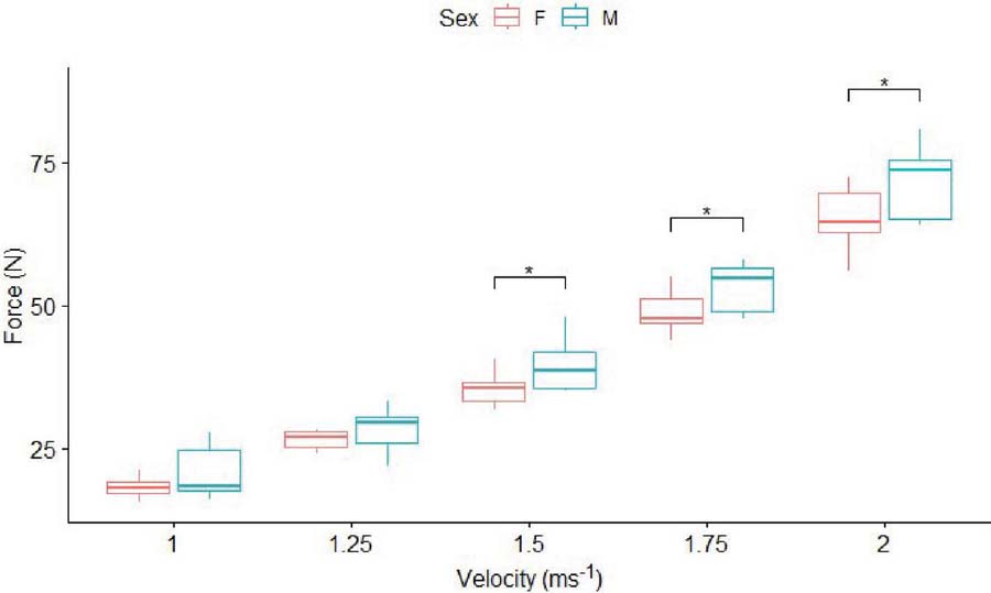
Figure 7 Box and whisker plots of passive drag measurements at different velocities for the male and female athletes. Significant contrasts between male and female average drag forces at each velocity are indicated by asterisks (* p 0.05, ** p 0.01, *** p 0.001).
Table 6(a): Summary table of ANOVA investigating contribution of sex and velocity, and their interaction, to measured drag force. df = between group degrees of freedom, df = within-group degrees of freedom, F = F-statistic (representing ratio of explained and unexplained variance according to the ANOVA model being tested), = partial eta-squared
| Effect | df | df | F | p | p.05 | |
| Sex | 1 | 8 | 3.318 | 0.106 | 0.293 | |
| Velocity | 4 | 32 | 712.885 | 0.001 | *** | 0.989 |
| Sex:Velocity | 4 | 32 | 1.605 | 0.197 | 0.167 |
Table 6(b): Average drag force for male vs female athletes at each towing velocity (expressed as mean standard deviation)
| Male Average | Female Average | ||
| Velocity (ms) | Passive Drag (N) | Passive Drag (N) | p (Female = Male) |
| 1.00 | 21.0 4.4 | 18.2 1.6 | 0.096 |
| 1.25 | 28.2 3.6 | 26.5 1.5 | 0.212 |
| 1.50 | 39.5 4.4 | 35.3 2.7 | 0.027 |
| 1.75 | 53.1 4.0 | 48.6 3.4 | 0.021 |
| 2.00 | 72.4 6.3 | 65.5 5.1 | 0.021 |
Analysis of variance indicated that only towing velocity significantly affected variance in measured force (p 0.001, Table 6b). Effect size analysis using partial-eta-squared ( proportion of variance explained by a given factor after accounting for variance explained by other factors) demonstrated that considerably higher proportion of variance was explained by velocity ( = 0.989) compared with either sex or the interaction between sex and velocity ( = 0.293 and 0.167 respectively).
The average passive drag was larger for males than females at each towing velocity but differences were only significant at the higher velocities (Figure 7), indicating sex is more likely to impact passive drag at higher velocities. Standard deviation was largest at 2 ms for both males and females, with female standard deviation steadily increasing with velocity. Standard deviation was more consistent for male athletes across the velocity ranges. An increase in variability with towing velocity is expected, as shown by the female athletes, as the drag differences caused by the varying size, shape, and body positions of athletes would be amplified as velocity increases. This is assuming each athlete maintains approximately the same body position across all towing velocities. For male athletes, the standard deviation did not always increase with velocity. Results indicate that it is possible the technique of the female athletes is more consistent than that of the males, due to less variation at each velocity. It is also possible that there is a larger range of male body types, which would result in an inflated value of standard deviation at lower velocities, although this would need further investigation.
Generally, the passive drag forces, shown in Table 6b, matched or were slightly lower when compared to existing literature of passive drag tows (Table 7).
Table 7 Comparison of experimental results with existing literature
| Male Average | Gatta | Gatta | |
| Velocity (ms) | Passive Drag (N) | et al. (N) [42] | et al. (N) [6] |
| 1.00 | 21.0 | 25 4 | 32.1 |
| 1.25 | 28.2 | 41 | 42.5 |
| 1.50 | 39.5 | 58 | 53 |
| 1.75 | 53.1 | 87 | 70 |
| 2.00 | 72.4 | 113 15 | 93 |
Results in literature tend to vary from approx. 20–25 N at 1.00 ms to 70–120 N at 2.00 ms [7]. The testing protocol of Gatta et al and this paper was very similar, with the main difference being the depth of the tow. Gatta et al used a slightly different force measurement device, namely a dynamometer, in order to record the forces. This slight decrease could be due to the athletes being towed at a depth of 1 m, whereas athletes were typically towed at surface level in other studies, giving rise to additional wave drag.
Other reasons for the differences between reported results and literature could be due to differences in body shape and size. The reasons stated for differences in results are speculative and would again need further investigation.
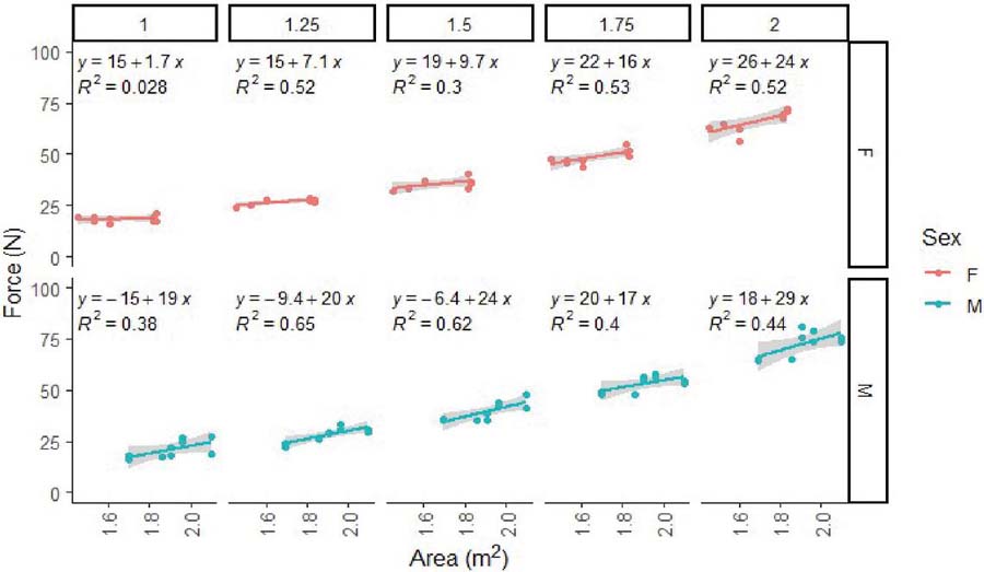
Figure 8 Measured force vs approximated surface area, stratified by velocity and sex. Equations describing lines of best fit (and associated coefficients of determination) are included for each combination of stratification levels above each line. Shaded regions around lines are 95% confidence intervals.
Prior to curve fitting according to the expected form of Equation (20) (i.e. ), further stratification of the relationship between velocity and towing force by approximated surface area and sex demonstrates that measured force was moderately correlated with surface area at most velocities (Figure 8). Athlete surface area was approximated based on a model proposed by Reading and Freeman [43]:
| (21) |
where m is the mass of the athlete in kilograms and h is the height of the athlete in meters. While sensitivity to area (indicated by the slope of each regression line) did not exhibit a pattern for male athletes (slopes oscillating between 19–29), sensitivity to area tended to increase more noticeably with velocity for female athletes (slopes monotonically increasing from 1.7–24).
Generally, these results show that passive drag at a given velocity tends to increase as surface area increases, in agreement with the work of Cortesi where drag increases with cross sectional area [44]. This is expected based on the drag equation shown in Equation (20). Correlation of surface area with passive drag force was mostly moderate at each velocity: ranged between 0.38–0.65 across the different velocities, with the exception of the slowest tow for female athletes ( at 1 ms).
In order to fully analyse results, a linear mixed-effects regression model was fitted to the physics-based assumption represented by Equation (21) earlier, i.e. assuming force is proportional to the square of velocity multiplied by athlete surface area. The analysis was also stratified by athlete sex, to enable estimation of separate drag coefficients for female and male athletes (Table 8). For the mixed-effects analysis, sex, surface area, and velocity were treated as fixed affects (i.e. assumed to affect the level of response) while participant ID was treated as a random effect (assumed to affect variability of the response, e.g. due to unmeasured subject-specific factors that accumulate in measurements during repeated testing of individuals across velocities and at each velocity).
Table 8 Summary table of mixed-effects regression analysis of drag force as a function of sex, surface area, and velocity. In mixed-effects analysis the conditional measures overall proportion of variance explained by both fixed and random effects, while the marginal measures proportion of variance explained by only fixed effects
| Parameter | 95% CI | p | Fit | |
| Sex (F): Area Velocity | 0. 0191 | (0.0184, 0.0199) | .001 | |
| Sex (M): Area Velocity | 0.0183 | (0.0177, 0.0189) | .001 | |
| R (conditional) | 0.98 | |||
| R (marginal) | 0.96 |
A higher drag coefficient was estimated for female athletes () relative to male athletes (). Interestingly, it appears the drag coefficient for female athletes is higher than males, implying that for the same surface area, females will exhibit higher passive drag at particular velocity values. This could be due to body composition or technique but would need further investigation.
The mixed-effects regression analysis demonstrated significant correlation (p 0.001) for both female and male athletes according to the assumption that drag force is a function of athlete surface area and the square of velocity (Table 8). The fixed effects (surface area, velocity, and sex), as represented by R (marginal), accounted for 96% of measured variance. Including the random effect due to unmeasured athlete-specific factors, as represented by R (conditional), accounted for only a further 2% of measured variance. The relatively small contribution to variance from the random effects term implies that in future a conventional regression model using only the fixed effects may be sufficient to explain many of the results.
Further Experimental Results: Surface vs Underwater Towing
Typically, passive drag tow tests are completed on the water surface. To help provide context to the current underwater results, a previous set of data collected by the authors (in which a limited number of surface tow tests were completed, based on the maximum swimming velocity of the athletes) were also analysed. A total of 14 passive drag tows were completed, with seven male athletes completing one towing velocity twice, corresponding to the maximum velocity recorded for said athlete during semi-tethered swimming. The semi-tethered equipment set up was almost identical, with the only major difference being that towing was completed on the surface and not at depth. The results of the surface trial are shown in Figure 9, in combination with the underwater results collected in the main experiment discussed in this paper. A key difference between the previous and current study is the athlete-specific specification of velocity in the surface study, which prevents direct contrasts at the controlled velocities used in the underwater study, which is evident from the lack of alignment between test velocities between the lower underwater tests and the upper surface tests in Figure 9.
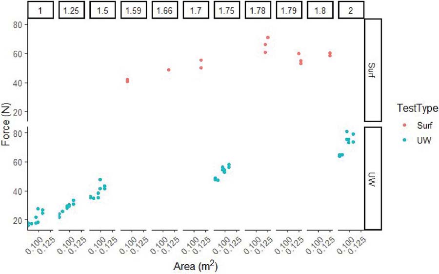
Figure 9 Scatter plot showing the relationship between passive drag and surface area, stratified by towing depth and towing velocity.
Ordinary least squares fitting of a quadratic velocity curve to the force data qualitatively demonstrates the expected relationship between force and velocity for both surface and underwater towing (Figure 10).
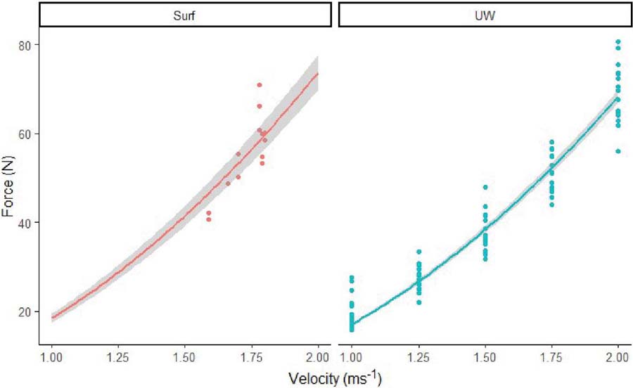
Figure 10 Plot of surface against underwater passive drag at different velocities with quadratic line of best fit applied.
From Figures 9 and 10, there is no clear difference in passive drag results between being towed underwater and on the surface. In order to further investigate and compare results, a more thorough surface tow test would have to be carried out, following the same protocol as used for the underwater towing tests. Similar to the underwater study, a mixed-effects regression analysis was completed using surface area and velocity as fixed effects and participant ID as the random effect (Table 9). Athlete sex was dropped from the analysis to allow test type (surface vs underwater) to be used to stratify estimates of drag coefficient for each test type.
Table 9 Summary table of mixed effects regression analysis of drag force as a function chest cross-sectional area and velocity; Type(Surf) implies surface tests and Type(UW) implies underwater tests
| Parameter | 95% CI | p | Fit | |
| Type (Surf): Area Velocity | 0. 0184 | (0.0179, 0.0200) | .001 | |
| Type (UW): Area Velocity | 0. 0182 | (0.0179, 0.0200) | .001 | |
| R (conditional) | 0.97 | |||
| R (marginal) | 0.94 |
Again, results show the significant correlation (p 0.001) of passive drag with the surface area and velocity of the athlete being towed. Estimated values for the drag coefficient for each test type were very similar (0.0184 for surface tests vs 0.0182 for underwater tests), indicating that test type does not seem to influence the average values of measured drag force. The large marginal R value again indicates that subject-specific factors other than athlete surface area, e.g. potential variations in technique, contribute very little to total variance compared to the fixed effects of surface area and velocity.
CFD Simulations
Primitive geometry validation cases
Beginning with the 2D cases, results for both turbulent models for low Reynolds 2D flows compared well to 2D cylinder experimental data [45] (Table 10). The results for k- simulations are more accurate, likely due to improved refinement levels. Results are also comparable with 2D CFD simulation results, with the results for the current study marginally lower [46].
Table 10 Drag coefficients of 2D cylinder at different levels of mesh refinement
| 2D | ||||||
| Cylinder | (low Re) | (low Re) | Existing Data | (high Re) | (high Re) | Existing Data |
| Refinement | (k-) | (k-) | (low Re) [45] | (k-) | (k-) | (high Re) [45] |
| Coarse | 2.27 | 2.42 | 2.40 | 0.83 | 0.91 | 1.05 – 1.20 |
| Medium | 2.21 | 2.39 | 2.40 | 0.43 | 0.89 | 1.05 – 1.20 |
| Fine | 2.15 | 2.36 | 2.40 | 0.18 | 0.98 | 1.05 – 1.20 |
Predictions begin to differ when investigating the high Reynolds number case. The k- turbulence model underpredicted the drag coefficient and became less accurate with increasing mesh refinement. In contrast, the k- predictions were considerably closer to existing experimental [45] and approximate simulation data [47]. The reason for improved predictions when using the k- model compared to the k- model could be due to the superior near-wall modelling properties of the k- model, although this would need further investigation.
For the 3D case only the k- model predictions are included (Table 11) as the increased computational requirements to create an appropriate mesh for the k- model prevented simulations from being set up for the latter model. For the low Reynolds number cases, the prediction error decreased with increased mesh refinement for the k- model, matching experimental data reasonably [48]. The drag coefficient for the high Reynolds number case fluctuated with increasing mesh refinement, with largest error predicted for the finest mesh, when compared to experimental literature [48]. Results for the coarse and medium cases were reasonable. These oscillations may be due to solving an unsteady flow problem with a steady flow solver, although this would need further investigation.
Table 11 Drag coefficients of 3D sphere at different levels of mesh refinement
| 3D Sphere | Cd | Cd | Lit Cd | Lit Cd |
| Refinement | (low Re) | (high Re) | Low Re [48] | High Re [48] |
| Coarse | 1.64 | 0.45 | 2.50 | 0.50 |
| Medium | 2.83 | 0.51 | 2.50 | 0.50 |
| Fine | 2.80 | 0.20 | 2.50 | 0.50 |
Passive drag simulation of streamlined swimmer
The results of the mesh convergence study for the passive drag simulations indicate convergence had not been achieved, but as previously stated, computational limitations hindered further investigation (Table 12 and Figure 11).
Table 12 Total Drag force of streamline geometry at different levels of mesh refinement
| 3D Passive Drag | Pressure Drag (N) | Viscous Drag (N) | Total Drag (N) |
| Coarse | 151.2 | 10.6 | 161.8 |
| Medium | 114.6 | 13.8 | 128.4 |
| Fine | 99.3 | 17.0 | 116.3 |
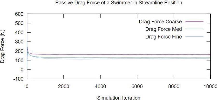
Figure 11 Convergence of passive drag force at different mesh refinement levels.
In order to compare the simulation results with the experimental results, cases were run for the finest mesh for each of the velocities used in the experimental study (Table 13 and Figure 12). The trends of the simulations are encouraging, with the total drag force, equivalent to passive drag, increasing with velocity. The results also show rate of growth of passive drag increases as the velocity increases (Figure 13), as expected from Equation (20) since the drag should scale with the square of velocity.
Table 13 Passive drag value on streamline geometry for changing velocity. Experimental drag refers to averages for male athletes standard deviations
| Velocity | Pressure | Viscous | Total | Experimental |
| (ms) | Drag (N) | Drag (N) | Drag (N) | Drag (N) |
| 1.00 | 26.3 | 4.9 | 31.2 | 21.0 4.3 |
| 1.25 | 40.2 | 7.3 | 47.5 | 28.2 2.8 |
| 1.50 | 56.9 | 10.1 | 67.0 | 39.5 4.3 |
| 1.75 | 76.7 | 13.3 | 90.0 | 53.1 3.8 |
| 2.00 | 99.3 | 17.0 | 116.3 | 72.4 6.7 |
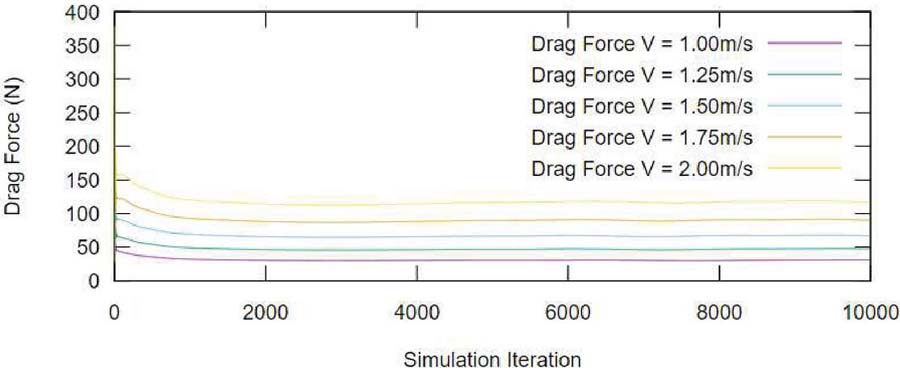
Figure 12 Convergence of passive drag force at different velocity values.
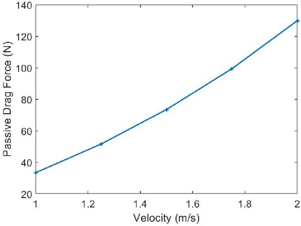
Figure 13 Increase of passive drag values with increase of velocity.
When compared to the experimental results and existing literature, the CFD simulations over-predict drag for a streamline position. Typical results from literature range from approx. 19.7 N at 1.00 ms to approx. 70–90 N at 2.00 ms [7], similar to the experimental results of this study (Table 6 and Table 12). A breakdown of existing interpolated results are included in Table 14.
Table 14 Comparison of computational results with existing literature
| Velocity | Male Average | Zaidi | Bixler |
| (ms) | Passive Drag (N) | et al. (N) [49] | et al. (N) [8] |
| 1.00 | 31.2 | – | – |
| 1.25 | 47.5 | – | – |
| 1.50 | 67.0 | 30 | 31.58 |
| 1.75 | 90.0 | 45 | 42.74 |
| 2.00 | 116.3 | 55 | 55.57 |
The values tend to vary significantly from study to study, likely due to the geometry used and set-up conditions. The surface area of the model used in this study was approx. 2.2 m, compared to a surface area of 1.859 m by Bixler et al. [8]. The frontal surface area of the geometry in this paper is unknown for comparison, but it is expected to be larger than that of Bixler. Due to this larger surface area, the passive drag results should be larger, as displayed by the results. With respect to geometry, the mesh used to represent the swimmer in the CFD simulations had arms that were more separated than was evident in the experimental study and some of the studies reviewed in the literature. When compared to a study by Zahn et al [50], where the athlete is in a position more similar to the geometry used in this study, i.e. with arms separated, the results match better (Table 15). Although results do match well, Zahn conducted simulations at the surface of the water, meaning the results could be slightly inflated and less comparable with results in the current analysis.
Table 15 Comparison of passive drag with existing literature for geometry with open arms
| Velocity (ms) | Zhan Passive Drag (N) [50] | Passive Drag (Current Analysis) (N) |
| 1.00 | 30.0 | 31.2 |
| 1.25 | 43.0 | 47.5 |
| 1.50 | 65.0 | 67.0 |
| 1.75 | 85.0 | 90.0 |
| 2.00 | 115.0 | 116.3 |
Zahn et al. also used a body fitted mesh in contrast to the immersed boundary mesh used above, which could also be responsible for the slight differences. Other differences could include the quality of the actual geometry used in simulations, as the geometry used by Zahn et al. appears to be more realistic when compared to the mesh used in this study [50].
The drag coefficient of the streamlined swimmer in the finest mesh case was approximately 0.12, an order of magnitude higher than the reported experimental drag coefficients found in the tow test. This implies that the difference in drag between simulated and experimental results could be caused by differences in drag coefficients of the CFD geometry when compared to human athletes, as the velocities and density are all approximately consistent when comparing experiments and simulations. It is also unlikely the wetted surface areas of the experimental cases, literature cases and computational analysis are the same, especially considering the limitations of reshaping the geometry. This could cause further error in the prediction of the passive drag force acting on a swimmer in a streamline position.
In order to display the sensitivity of passive drag to a change in surface area, the surface area of the swimming geometry was approximately doubled, from 2.20 m to 4.44 m, using the ‘blender’ software. The change in the wetted surface area, which will be the main surface area that impacts drag, is unknown but expected to have increased substantially. Included in Table 16 are results for a coarse mesh, with the minimum cell size equal to the minimum cell size of the standard geometry coarse mesh detailed above, but a slightly larger refined domain, to account for the increased geometry size. This comparison case has been run with an inlet velocity of 2 ms, with all other initial conditions and numerical schemes remaining the same as the unscaled coarse case.
Table 16 Comparison of passive drag results when comparing standard geometry with scaled geometry
| Standard Geometry Mesh | Scaled Up Geometry Mesh | |
| Cell Count | 1097084 | 5553480 |
| Total Passive Drag (N) | 161.8 | 285.2 |
Results for passive drag for the scaled geometry were larger when compared to the standard geometry, as expected due to the surface area term in the drag equation. Results do show that the utilised immersed boundary surface method is able to cope with different geometry characteristics, which is promising for future work in the field.
The relative consistency of a streamline position between athletes makes this a good choice for validating computational simulations. However, this consistency makes it difficult to suggest feedback in order to reduce one’s passive drag. Nevertheless, one suggestion that could be made is to encourage coaches to suggest athletes remain in a ‘tight’ streamline position, as shown in Figure 3, and avoid a ‘loose’ streamline position, similar to the position shown in the CFD geometry in Figure 6.
The comparison of passive drag within this study is a first step in future drag predictions in swimming, with the long-term aim being to predict the active drag profile of an athlete via CFD (using the immersed boundary surface method proposed in this study) and experimental means (as completed by Haskins et al. [51]). Active drag is defined as the change in drag across a stroke cycle when an athlete is actively swimming through the water, for example during Freestyle swim. Provided it is possible to alter the kinematics of a swimming geometry quickly for use in CFD, it would potentially be possible to use CFD simulations to suggest technical changes that could allow the reduction of active drag for an athlete. The limitations of performing this task would need further investigation, although the work completed in the current study demonstrates this would be a natural next step in the research.
There are several notable novel aspects of this work. This is the first study, to the authors’ knowledge, that uses a finite volume with immersed boundary surface method to predict passive drag in swimming, thus demonstrating a novel approach to this challenging problem. This work is also one of the few studies that investigates the passive drag of an athlete using more than one methodology, i.e. towing and CFD, allowing for immediate validation of the method. The use of the 1080 Sprint as a method to measure passive drag has also been completed for a first time, based on the current published literature, although other research groups are currently using this method, namely Ulster University. The measurement of passive drag via the towing method whilst completely underwater is also uncommon in literature, with this research adding to the field. Comparing these results to surface tows, as outlined in the results section, is also uncommon within the existing literature in the field.
Conclusions
There are a number of conclusions that can be drawn from the work completed in this paper. Firstly, the experimental results showed and confirmed the important influence of velocity on the passive drag of an athlete. The results also confirmed, in line with literature, that biological sex and athlete surface area also have an important role to play in the passive drag produced when in a streamlined position.
Secondly, although there are some over-predictions when using the immersed boundary method to find the drag coefficients of primitive geometries, drag coefficient results are reasonable, especially in 3D and in 2D when using the k- SST instead of the k- model. Results are likely to improve in 3D with the implementation of the k- SST model and by using a smoother 3D sphere. The immersed boundary method estimated reasonable results for drag produced by a swimmer in streamline, especially when results were compared to a similar positioned geometry in literature. The results also indicate that the wetted surface area and drag coefficient could be responsible for the differences in computational solutions when compared with data found experimentally and in literature.
Overall, using the immersed boundary method to predict drag coefficients of primitive shapes and the passive drag of an athlete was promising, although somewhat over-predictive. CFD results do show the general trend of data, as found experimentally, meaning that feedback can still be suggested based on results with the disclaimer that collected CFD results are likely to be over-predictive. The results indicate that the immersed boundary method could be useful in removing body fitted meshing issues, whilst still providing reasonably accurate, if not slightly over predictive, results. This has the potential for further application in moving body problems.
Data Availability
Anonymised datasets used during analysis are available from one of the named authors, Alex Lennon, on reasonable request. Video footage of the experiments will not be made available at any time, in accordance with ethics approval.
Abbreviations
| 2D | – | 2 Dimensional |
| 3D | – | 3 Dimensional |
| CFD | – | Computational Fluid Dynamics |
| IBM | – | Immersed Boundary Method |
Acknowledgements
The authors would like to thank all study participants and coaches for their contribution to the study. The authors would also like to thank Ulster University and Lisburn City Swimming Club for their expertise and support throughout the study. The authors would also like to thank those who helped with result collection during the main experiment.
Funding
The authors would like to thank and acknowledge funding from the Department for the Economy that made this study possible.
Contributions
A.H. developed the study concept and designed the experimental setting in conjunction with A.L., C.M. and D.C. A.H. recruited the participants with A.H., C.M. and R.K. collecting the data. C.M. and R.K. provided expertise for the 1080 Sprint. A.H. and A.L. post processed and analysed the experimental data with assistance from R.K. A.H. completed the computational simulations with significant guidance from D.C. A.H. post processed the computational results with significant guidance provided by D.C. A.H. wrote the first draft with alterations advised by A.L, and D.C. A.H. wrote the revisions with alterations suggested and in part completed by A.L.
Competing Interests
The authors declare no competing interests.
Corresponding Author
Correspondence to Alex Lennon
References
[1] Voronstov, A. R., Rumyanstev, V.A. (2008). Resistive Forces In Swimming. In Biomechanics in SportBlackwell Science Ltd. https:/doi.org/10.1002/9780470693797.ch27
[2] Payton, C., Hogarth, L., Burkett, B., van de Vliet, P., Lewis, S., and Oh, Y. T. (2020). Active Drag as a Criterion for Evidence-based Classification in Para Swimming. Medicine and Science in Sports and Exercise, 52(7), 1576–1584. https:/doi.org/10.1249/MSS.0000000000002281.
[3] Barbosa, T. M., Ramos, R., Silva, A. J., and Marinho, D. A. (2018). Assessment of passive drag in swimming by numerical simulation and analytical procedure. Journal of Sports Sciences, 36(5), 492–498. https:/doi.org/10.1080/02640414.2017.1321774.
[4] Dubois-Reymond, R., 1905. Zum Physiologie des Schwimmens. Archive fur Anatomie und Physiologie (Abteilung Physiologie). XXIX, 252–279.
[5] Clarys JP. Hydrodynamics and electromyography: ergonomics aspects in aquatics. Appl Ergon. 1985 Mar;16(1):11–24. doi: 10.1016/0003-6870(85)90143-7. PMID: 15676530.
[6] Gatta G, Cortesi M, Zamparo P. The Relationship between Power Generated by Thrust and Power to Overcome Drag in Elite Short Distance Swimmers. PLoS One. 2016 Sep21;11(9):e0162387. doi: 10.1371/journal.pone.0162387. PMID: 27654992; PMCID: PMC5031421.
[7] Scurati, R., Gatta, G., Michielon, G., and Cortesi, M. (2019). Techniques and considerations for monitoring swimmers’ passive drag. Journal of Sports Sciences, 37(10), 1168–1180.
[8] Bixler, B., Pease, D., and Fairhurst, F. (2007). The accuracy of computational fluid dynamics analysis of the passive drag of a male swimmer. Sports Table 5. Biomechanics, 6(1), 81–98.
[9] Narita, K., Nakashima, M., and Takagi, H. (n.d.). Title: Developing a methodology for estimating the drag in front-crawl swimming at various velocities.
[10] Chatard, J. C., and Wilson, B. (2008). Effect of fastskin suits on performance, drag, and energy cost of swimming. Medicine and Science in Sports and Exercise, 40(6), 1149–1154. https:/doi.org/10.1249/MSS.0b013e318169387b.
[11] Hay, J. G., and Carmo, J. (1995). Swimming techniques used in the flume differ from those used in a pool. Paper presented at the XV International Society of Biomechanics, Finland: Congress, Jyväskylä.
[12] Wilson, B., Takagi, H., and Pease, D. (1998). Technique comparison of pool and flume swimming. Paper presented at the VIII International Symposium on Biomechanics and Medicine in Swimming,
[13] Jyväskylä, Finland. Bilo, D., and Nachtigall, W. (1980). A simple method to determine drag coefficients in aquatic animals. In J. exp. Biol (Vol. 87).
[14] Kjendlie, P. L., and Stallman, R. K. (2008). Drag characteristics of competitive swimming children and adults. Journal of Applied Biomechanics, 24(1), 35–42. https:/doi.org/10.1123/jab.24.1.35.
[15] Mollendorf, J. C., Termin, A. C., Oppenheim, E., and Pendergast, D. R. (2004). Effect of swim suit design on passive drag. Medicine and Science in Sports and Exercise, 36(6), 1029–1035. https:/doi.org/10.1249/01.MSS.0000128179.02306.57.
[16] Barbosa, T. M., Costa, M. J., Morais, J. E., Morouço, P., Moreira, M., Garrido, N. D., Marinho, D. A., and Silva, A. J. (2013). Characterization of speed fluctuation and drag force in young swimmers: A gender comparison. Human Movement Science, 32(6), 1214–1225. https:/doi.org/10.1016/j.humov.2012.07.009.
[17] Takagi, H., Nakashima, M., Sato, Y., Matsuuchi, K., and Sanders, R. H. (2016). Numerical and experimental investigations of human swimming motions. In Journal of Sports Sciences (Vol. 34, Issue 16, pp. 1564–1580). Routledge. https:/doi.org/10.1080/02640414.2015.1123284.
[18] von Loebbecke, A., Mittal, R., Fish, F., and Mark, R. (2009). Propulsive efficiency of the underwater dolphin kick in humans. Journal of Biomechanical Engineering, 131(5). https:/doi.org/10.1115/1.3116150.
[19] von Loebbecke, A., Mittal, R., Mark, R., and Hahn, J. (2009). A computational method for analysis of underwater dolphin kick hydrodynamics in human swimming. Sports Biomechanics, 8(1), 60–77. https:/doi.org/10.1080/14763140802629982.
[20] Döhler, J. E. (n.d.). An Analysis of the Immersed Boundary Surface Method in foam-extend. www.chalmers.se.
[21] opensource. (2022). Foam-Extend-5.0.
[22] S.V Patankar, D. B. S. (1972). A calculation procedure for heat, mass and momentum transfer in three-dimensional parabolic flows. International Journal of Heat and Mass Transfer, 15(10), 1787–1806.
[23] W. Malalasekera and H. Versteeg. An introduction to computational fluid dynamics: the finite volume method. Pearson Prentice Hall, 2007
[24] B. Launder and D. Spalding. “The numerical computation of turbulent flows”. In: Computer Methods in Applied Mechanics and Engineering 3.2 (1974), pp. 269–289. issn: 0045-7825. doi: 10.1016/0045-7825(74) 90029-2. url: https:/www.sciencedirect.com/science/article/pii/0045782574900292.
[25] F. Menter, M. Kuntz, and R. Langtry. “Ten years of industrial experience with the SST turbulence model”. In: Heat and Mass Transfer 4 (Jan. 2003).
[26] Peskin CS. 1972. Flow patterns around heart valves: a digital computer method for solving the equations of motion. PhD thesis. Physiol., Albert Einstein Coll. Med., Univ. Microfilms. 378:72–30.
[27] H. Jasak. “Immersed boundary surface method in foam-extend”. In: The 13th OpenFOAM Workshop (OFW13) (June 2018), pp. 55–59.
[28] OpenFoam. (2016). Forces. OpenFOAM: User Guide V2112. https:/www.openfoam.com/documentation/guides/latest/doc/guide-fos-forces-forces.html.
[29] 1080 Motion. (n.d.). https:/1080motion.com/.(Conducted: January 2022)
[30] codethislab. (2020). Male Animated Swimmer HQ 001 3D. Shutterstock.
[31] Mathworks. (2022). MATLAB – findpeaks (No. R2022b). MathWorks Inc., USA.
[32] Gonjo, T., and Olstad, B. H. (2022). Reliability of the active drag assessment using an isotonic resisted sprint protocol in human swimming. Scientific Reports, 12(1). https:/doi.org/10.1038/s41598-022-17415-5.
[33] R Core Team. 2023. R: A Language and Environment for Statistical Computing. Vienna, Austria: R Foundation for Statistical Computing. https:/www.R-project.org/.
[34] Wickham, Hadley. 2023. Tidyverse: Easily Install and Load the Tidyverse. https:/CRAN.R-project.org/package=tidyverse.
[35] Wickham, Hadley, Mara Averick, Jennifer Bryan, Winston Chang, Lucy D’Agostino McGowan, Romain François, Garrett Grolemund, et al. 2019. “Welcome to the tidyverse.” Journal of Open Source Software 4 (43): 1686. https:/doi.org/10.21105/joss.01686.
[36] Schloerke, Barret, Di Cook, Joseph Larmarange, Francois Briatte, Moritz Marbach, Edwin Thoen, Amos Elberg, and Jason Crowley. 2021. GGally: Extension to Ggplot2. https:/CRAN.R-project.org/package=GGally.
[37] Kassambara A (2023). rstatix: Pipe-Friendly Framework for Basic Statistical Tests. R package version 0.7.2, https:/CRAN.R-project.org/package=rstatix.
[38] Bates, Douglas, Martin Mächler, Ben Bolker, and Steve Walker. 2015. “Fitting Linear Mixed-Effects Models Using lme4.” Journal of Statistical Software 67 (1): 1–48. https:/doi.org/10.18637/jss.v067.i01.
[39] Bates, Douglas, Martin Maechler, Ben Bolker, and Steven Walker. 2023. Lme4: Linear Mixed-Effects Models Using Eigen and S4. https:/github.com/lme4/lme4/.
[40] Tom Roosendale. (2021). Blender.
[41] Wang Q, Wang Z. Quantitative Analysis of Drag Force for Task-Specific Micromachine at Low Reynolds Numbers. Micromachines (Basel). 2022 Jul 18;13(7):1134. doi: 10.3390/mi13071134. PMID: 35888951; PMCID: PMC9317653.
[42] Gatta, G., Cortesi, M., and di Michele, R. (2012). Power production of the lower limbs in flutter-kick swimming. Sports Biomechanics, 11(4), 480–491. https:/doi.org/10.1080/14763141.2012.670663.
[43] Reading, B.D., Freeman, B., 2005. Simple formula for the surface area of the body and a simple model for anthropometry. Clinical Anatomy 18, 126–130. https:/doi.org/10.1002/ca.20047.
[44] Cortesi M, Gatta G, Michielon G, Di Michele R, Bartolomei S, Scurati R. Passive Drag in Young Swimmers: Effects of Body Composition, Morphology and Gliding Position. Int J Environ Res Public Health. 2020 Mar 18;17(6):2002. doi: 10.3390/ijerph17062002. PMID: 32197399; PMCID: PMC7142561.
[45] Panton, R., Incompressible Flow. 4 edition, Published 2013.
[46] Sheard, G. J., Hourigan, K., and Thompson, M. C. (2005). Computations of the drag coefficients for low-Reynolds-number flow past rings. Journal of Fluid Mechanics, 526, 257–275. https:/doi.org/10.1017/S0022112004002836.
[47] Yuce, M. I., and Kareem, D. A. (2016). A numerical analysis of fluid flow around circular and square cylinders. Journal – American Water Works Association, 108(10), E546–E554. https:/doi.org/10.5942/jawwa.2016.108.0141.
[48] Almedeij, Jaber. (2008). Drag Coefficient of Flow Around a Sphere: Matching Asymptotically the Wide Trend. Powder Technology - POWDER TECHNOL. 186. 218–223. 10.1016/j.powtec.2007.12.006.
[49] Zaïdi, H., Fohanno, S., Taïar, R., and Polidori, G. (2010). Turbulence model choice for the calculation of drag forces when using the CFD method. Journal of Biomechanics, 43(3), 405–411. https:/doi.org/10.1016/j.jbiomech.2009.10.010.
[50] Zhan, J. M., Li, T., Chen, X., Li, Y., and Wai, W. O. (2015). 3D numerical simulation analysis of passive drag near free surface in swimming. China Ocean Engineering, 29(2), 265–273.
[51] Haskins, A., McCabe, C., Kennedy, R., McWade, R., Lennon, A. B., and Chandar, D. (2023). A novel method of determining the active drag profile in swimming via data manipulation of multiple tension force collection methods. Scientific Reports, 13(1). https:/doi.org/10.1038/s41598-023-37595-y.
Biographies

Alex Haskins is a PhD student in Aerospace Engineering at Queen’s University Belfast. Alex’s PhD research, commenced in 2021, investigates drag in human frontcrawl swimming, quantified via computational and experimental means. Before commencing his PhD research, Alex graduated from Queen’s University Belfast in 2021 with an MEng in Aerospace Engineering (First Class Honours). Alex is growing his research portfolio throughout his PhD, with a previous publication in July of 2023 entitled ‘A novel method of determining the active drag profile in swimming via data manipulation of multiple tension force collection methods’.

Carla McCabe is a Senior Lecturer in Sport and Exercise Biomechanics at Ulster University. Carla’s research interests are in human movement performance, specifically within an aquatic environment. Since 2008, Carla has developed extensive expertise in swimming biomechanics as evidenced by her international research portfolio, publication outputs and peer-review engagement across numerous Sport Science and Biomechanics journals. Carla graduated from the University of Limerick (2003) with a BSc Sports and Exercise Science degree (First Class honours). Subsequently, she was awarded a scholarship and completed her PhD at the University of Edinburgh (2008) investigating the effect ‘race pace’ had on three-dimensional kinematics and linear kinetics within sprint and distance specialist swimmers.

Ryan Keating is currently a full-time PhD researcher at Ulster University, investigating load-velocity profiling in swimming. In 2020, Ryan completed an MSc in Strength & Conditioning at Ulster University. Ryan is an accredited strength & conditioning coach through the UK Strength & Conditioning Association with coaching experience in able-bodied and para-swimming, wheelchair basketball, judo, para-badminton, sailing, lawn bowls, rugby, Gaelic football, football and futsal. Ryan’s research interests include strength diagnostics for sport performance.

Alex Lennon is a senior lecturer in the School of Mechanical & Aerospace Engineering in Queen’s University, Belfast. His research interests include orthopaedic and cardiovascular biomechanics, tissue mechanics, biomaterials, medical device testing and analysis, mechanobiology of cells and tissues, and polymer mechanics and processing. After completing his undergraduate degree in Mechanical Engineering in University College Dublin, Alex worked as a research assistant and consultant engineer for a medical device campus spin-out company from University College Dublin’s Bioengineering Research Centre before undertaking and completing a Ph.D. in Bioengineering in Trinity College Dublin. Between his Ph.D. and moving to Queen’s University Belfast, he was lead technical developer for an Enterprise Ireland funded spin-out project to develop software for pre-operative planning of total hip replacement using patient-specific simulation of implant loosening and subsequently worked as a research fellow in Trinity College Dublin’s Centre for Bioengineering on projects to link biomechanical simulation tools with health informatics systems and develop computational tools for cell and tissue mechanobiology.

Dominic Chandar is currently a Computational Engineer at Luminary Cloud, with a diverse background in academia and research. From 2019 to 2021, Dominic served as a lecturer in the School of Mechanical and Aerospace Engineering at Queen’s University Belfast. Prior to that, Dominic was a scientist at the Agency for Science, Technology, and Research (A*STAR) in Singapore from 2013 to 2019. Dominic’s postdoctoral work, conducted between 2010 and 2013 at the University of Wyoming, focused on High Performance Computing for Computational Fluid Dynamics (CFD). Dominic earned his PhD in Computational Engineering from Nanyang Technological University’s School of Mechanical and Aerospace Engineering in Singapore (2006–2010). Earlier in Dominic’s career, he worked as a scientist in India’s Defence Research and Development Organisation (2004–2005) and completed a Master’s in Aerospace Engineering at the Indian Institute of Science, Bangalore (2002–2004).
European Journal of Computational Mechanics, Vol. 33_3, 255–294.
doi: 10.13052/ejcm2642-2085.3333
© 2024 River Publishers