Influence of Thermal Cycle on Viscoelastic Material Response
Priyanka Samal and Shantanu S. Mulay∗
Structural Mechanics Group, Department of Aerospace Engineering, Indian Institute of Technology Madras, Chennai – 600036, India
E-mail: ssmulay@iitm.ac.in
*Corresponding Author
Received 14 March 2025; Accepted 15 April 2026
Abstract
The present work aims to study the temperature cycle influence on a general viscoelastic (VE) material constitutive response. The time-dependent behaviour of VE material is modelled by Prony exponential series. A novel method, providing non-negative Prony coefficients, is used and successfully validated against various creep and relaxation experiment results. Displacement control experiments (relaxation) are difficult for stiff materials; load control experiments (creep) are thus performed in general. It is, therefore, essential to correctly convert creep compliance into relaxation modulus and vice versa. A correct inter-conversion novel method is thus derived in detail and successfully validated against various experimental results. A time-temperature superposition (TTS) is used to obtain a master curve for VE material by horizontal shift factors. Williams–Landel-Ferry equation constants are computed to obtain VE material properties at any temperature value within the available experimental range by linearising horizontal shift factors. The correctness of these constants is validated in a novel manner, thus highlighting the limitation of the linearisation process, which is generally adopted in the literature. The temperature dependence of VE material is finally coupled with a VE stress update algorithm through pseudo-time concept (without considering damage and ageing).
Keywords: Williams–Landel-Ferry constants, time-temperature superposition, viscoelastic, Prony coefficients, master curve, shift factor.
1 Literature review
1.1 Viscoelastic Material
Viscoelastic (VE) materials show both, elastic and viscous behaviors when subjected to loading, and their applications are seen in many areas, such as in rubber, automobile, aerospace, sports equipment, and engineering industries [1, 2, 3, 4]. The study of VE response is also extended in the medical field, as human skin and bones also show VE behaviour [5, 6], where the stress-strain relation depends on both, the time and temperature variables. Solid rocket propellants (SRP) behave as VE materials, and they are designed for a long-term storage period that exposes them to the local thermal cycles according to the climate and location [7, 8]. The service life of asphalt pavement is usually significantly affected by the temperature, with a daily variation in thermal cycle acting as a key environmental factor. High temperature cycle usually causes fatigue damage, while low temperature often leads to transverse cracks due to increase in material brittleness [9]. Turbine blades, heat exchanger, furnace lining, and exhaust systems (using VE materials) also undergo high temperature cycles during their service life, it is thus highly important to understand their VE behaviour at different temperatures.
1.2 Prony Coefficients and Inter-Conversion
The material response of VE materials is generally obtained from experiments, such as the relaxation and creep tests that are expressed in terms of Prony series. Relaxation and creep behaviors are two aspects of the same material, thus having some mathematical relations between them. This mathematical relation [4, 10], between creep and relaxation, allows their inter-conversion (creep compliance to relaxation modulus and vice versa). The necessity of inter-conversion method also arises, as it is not always possible to perform all the experiments to get the material behaviour. It is sometimes difficult to do the strain control experiment, i.e., relaxation test for stiff material, whereas the stress control experiment (creep test) becomes convenient. In such cases, the relaxation function can be obtained from the creep test by inter-conversion method.
1.3 Time-Temperature Superposition
The VE material shows time-temperature equivalence, i.e., the VE behaviour at one temperature can be related to that at another temperature by a change in the time scale [11]. The time-temperature transformation is thus done by a horizontal shift factor plotted on a logarithmic scale. The resulting curve (at a reference temperature), superimposing the results at different time and temperatures, is called the master curve. The Williams–Landel-Ferry equation (see [12]) gives a mathematical relation between the shift factor and temperature. The importance of master curve can be understood in many aspects. It is difficult to have a long-term test data of VE material, as testing would take a long time, and it may also affect the manufacturing process. Testing of VE material can be done at multiple test temperatures for a short time period, instead of doing the test at a particular temperature for a long time. The long-term behaviour of VE material can be predicted or interpolated, at different temperatures, from test results by the time-temperature superposition (TTS) principle. The behaviour of VE material can be predicted, at different times and temperatures, from the master curve (time range in which the experimental data is available), thus employing a limited set of experimental data [13, 14]. Several studies have done in the literature to obtain a master curve providing a long-term VE material response and finding WLF constants. It is though observed that the obtained WLF constants are not further verified while obtaining the appropriate VE material behaviour at any random temperature, which becomes important sometimes, as demonstrated in the subsequent sections.
1.4 Motivation
The first motivation of present work is to provide a simple process to shift VE material behaviour to a reference temperature while obtaining the master curve. The master curve is then validated against the available long-term experimental material behaviour. The second motivation is to verify WLF constants with experimental behaviour, so that WLF constants can be further used to obtain VE material behaviour at any temperature.
1.5 Novelties and contribution
A simple process, to obtain the master curve and WLF constants, is firstly proposed such that proper shifting of VE material response is achieved. The proposed approach is further validated against the available various experimental results in the literature. The proposed approach is then secondly coupled with VE material stress update formulation incorporating the TTS.
This paper is organized as follows. A brief description of Prony fit and inter-conversion of VE material properties is given in Section 2.1. A simple method is described in detail to obtain the master curve by TTS in Section 1. The WLF equation and how to obtain WLF constants are explained in Section 2.3. The numerical details to obtain stress in pseudo time is given in Section 3.1. The results and validation with the experimental data are finally presented in Section 4.
2 Theoretical Formulations Description
Various formulations, required in the present work, are given in this section.
2.1 Prony Fit and Inter-Conversion
The relaxation experimental data can be fitted in Prony series as
| (1) |
where is the relaxation modulus function of time , are total Prony series terms, is the long-time equilibrium modulus (as ), and and are values of Prony coefficient and relaxation time, respectively. The creep response, similar to the relaxation, can be fitted in another Prony series as
| (2) |
where is the creep compliance function of time , are the number of Prony terms, is a compliance at , and and are values of Prony coefficient and creep parameter, respectively. The correlation between relaxation and creep response is given as
| (3) |
where is a convolution function. Two extreme points, initial time () and long-time (), are given as
| (4) |
where inverse relation exists. The mathematical relations, given in Equations (3) and (4), allow the inter-conversion process. If one of the material responses is known in the time-space, the other response can be computed by solving Equation (3) [10].
2.2 Construction of Master Curve
The literature [16, 14, 13], available to the authors, is not very clear about the possible steps involved in the construction of VE material master curve, even though it has been used by many researchers for a very long time. The steps involved in the construction of VE material master curve are thus explained in details in this section, resulting in a physically realistic master curve, to give a better clarity to the readers. It is important to note here that the temperature is kept constant during the relaxation (or creep) experiment, such that the obtained response curve corresponds to the temperature . It may be possible that the temperature may be changing with time during the relaxation (or creep) experiment, which may not serve as a right input experiment while computing the horizontal shift factors in this section (and the subsequent computation of WLF equation constants).
Relaxation or creep experimental data are generally distorted, noisy, and duplicated; it is thus necessary to find the respective Prony series coefficients and plot smooth curves for relaxation or creep test for each temperature before proceeding any further (this step also helps in parametrization of all the curves rather than dealing with the raw data). We then choose a reference temperature, preferably in-between the available experimental temperature range, to get a more accurate master curve at the chosen reference temperature. The master curve is obtained by horizontally shifting the experimental material response curves to the chosen reference temperature in the logarithmic time scale. It is always likely that the relaxation curve goes from bottom to top (along the axis values) in the logarithmic scale as the temperature decreases (violation of this condition imply that the experimental results are either not correct or VE material of interest may not be obeying time-temperature superposition principle), as seen in Figure 4(a) [same value of relaxation modulus is reached sooner in time at high temperature comparing with the low temperature, which is a classical thermo-rheologically simple (TRS) material behaviour]. The creep compliance curves demonstrate an inverse behaviour as seen in Figure 6(a). The relaxation response curves, above the reference temperature, are thus shifted towards the right, and below the reference temperature, are shifted towards the left while obtaining the shift factor log, where and are any general- and reference temperature values, respectively, and all the response curves are converted to logarithmic scale. Consider the starting data point of response curve at temperature if is true, and consider the last data point of response curve at temperature if is true while computing the shift factor log.
Suppose there are three relaxation curves (in logarithmic scale) at the temperatures and 30 degrees, and 20C is taken as a reference temperature (C). Consider the last data point on C curve [] and horizontally project it on the master curve (at C) to obtain log. There may or may not be any valid data point on C curve (during horizontal projection process), corresponding to the ending data point of C curve, then one can use an interpolation to obtain (else sometimes extrapolation is required if the projected point on the reference temperature curve is going beyond the reference curve range). Now, consider the first data point on 30C curve [] and horizontally project it on the master curve (at C) to obtain log. One can again use interpolation (or extrapolation) while obtaining in the horizontal projection process of shift factor log computation.
The flowchart, to compute the shift factor for a response curve at any temperature, is given in Figure 1 (All the response curves and shift factors are in the logarithmic scale). Similar procedure is applicable for both, the relaxation and creep, curves. Physically shift all the response curves horizontally at the reference temperature once all the shift factors are computed thus resulting in a single curve, the master curve, describing the long-term VE material behaviour at the reference temperature.
The computed shift factors are also used to obtain WLF equation constants in the following section.
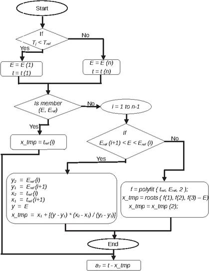
Figure 1 Flowchart to compute the horizontal shift factor in linear VE materials (TRS materials).
2.3 WLF Equation Parameters Computation
WLF equation is an empirical relation that relates to TTS principle by shift factor as [11]
| (5) |
where is a shift factor, which is a function of temperature ( itself may be a function of time ). The variables, and , are WLF constants that need to be determined from the shift factors obtained by TTS principle. The response curves, for at least three different temperature values, are required while computing and in Equation (5). The WLF equation constants are obtained by linearising Equation (5) as
| (6) |
where an inverse is taken in Equation (5), and the terms are simplified ( is used, without using time , for the sake of simplicity). The Equation (6) is in the form of a straight line, , where, , slope , , and the axis intercept . The material response curves, corresponding to at least three different temperature values, are required to ensure that at least two shift factors are known to obtain two WLF constants from Equation (6) (minimum two points are required to obtain a straight line). Plot Equation (6) using known shift factors (as explained in the previous Section 2.2), and fit a straight line by least square minimization. The slope and axis intercept can be used to obtain and .
The WLF constants can also be obtained directly by MATLAB® command fittype employing Equation (5), which fit the results in the least square manner. It is though noticed that and constants obtained by Equation (6) predict the stress response better than the ones obtained by fittype command employing Equation (5).
2.4 Pseudo Time Introduction in VE Material Stress Update Process
It is assumed in TRS VE materials that the temperature dependency is only through the relaxation time as [11]
| (7) |
where and are the relaxation time at reference temperature and the shift factor corresponding to temperature , respectively [computed as described in Section 2.2 or by Equation (5)]. The objective of using Equation (7) is that the temperature-dependent elastic Young’s modulus , given in Equation (1), can be directly computed by and at the reference temperature ( at ). It is thus not required to compute Prony parameters at every temperature as long as the reference temperature values are known. This statement will be explored more in details in the results and discussion section (Section 4). The modified Equation (1) is given as
| (8) |
where is a modified time called pseudo time given as
| (9) |
It can be seen from Equation (8) that resulting in . The Equations (8) and (9) are only correct when the temperature remains constant during the whole experiment. The temperature usually varies in real applications, the pseudo time is thus expressed in the integral form as
| (10) |
where represents the temperature function (of time ), and is a dummy time variable. The detailed discussion of coupling Equation (10) with VE stress update, given in Equation (12), is given in [11] (pseudo-time integration when temperature is a function of time ).
2.5 VE Material Stress Update
When the temperature effect is not considered, the constitutive response of linear VE material is generally given by a generalized Maxwell model with Maxwell elements as [11]
| (11) |
where is the stress, is the total strain and is the strain rate. The stress is given, including the temperature effect, as
| (12) |
where is given by Equation (7).
The numerical implementation details of the presented formulation are briefly discussed in the next section for the sake of completeness.
3 Numerical Integration
A discretized time step , in the interval , is introduced in Equation (11), and the strain rate is replaced as ). The integral part of Equation (11) can be given as [11]
| (13) |
The recursive internal history variable, by Equation (13), can be given as [11]
| (14) |
The stress, in Equation (11), is finally given in the discretized form as [11]
| (15) |
The history variable in terms of pseudo time is given as [11]
| (16) |
where is pseudo time increment given as
| (19) |
and is mid-point pseudo time increment given as
| (20) |
The shift factor can be computed by Equation (5) after obtaining the constants and as discussed in Section 2.3.
If temperature is constant during the experiment, the stress update is performed by Equations (13)–(15) using Equation (7) and employing all the material properties at the reference temperature in Equations (13)–(15). If temperature is varying with time , the stress update is performed by Equation (15), where is computed by Equations (16)–(20) and employing all the material properties at the reference temperature in Equations (15)–(20). The stress update procedure is consolidated in Box 3.1 for a quick reference.
Box 3.1: VE material stress update steps
Given: initial values, , , , or , , , WLF constants, and material parameters
Step 1: compute current strain and current time , (for , )
Step 2: compute pseudo time increment and mid-point pseudo time increment as Equations (19) and (20)
Step 3: compute history variable by Equation (16)
Step 4: compute stress by Equation (15)
The numerical implementation results, of the presented formulations, are discussed in the next section.
4 Results and Discussion
Curve fitting, for relaxation modulus and creep compliance, is done ensuring non-negative Prony series coefficients, and is validated against the experimental data taken from [14, 10] as shown in Figures 2(a) (relaxation fitting) and 2(b) (creep fitting). The inter-conversion method, given in Equation (3), is validated with the experimental result ([15]) as shown in Figure 3(a) by following the steps mentioned in Figure 3(b).
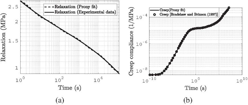
Figure 2 Prony fit to experimental data: (a) relaxation Prony fit [14], and (b) creep Prony fit [10].
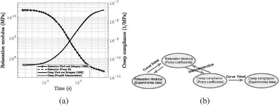
Figure 3 Inter-conversion of material behaviour: (a) inter-conversion Prony fit [15], (b) inter-conversion process.
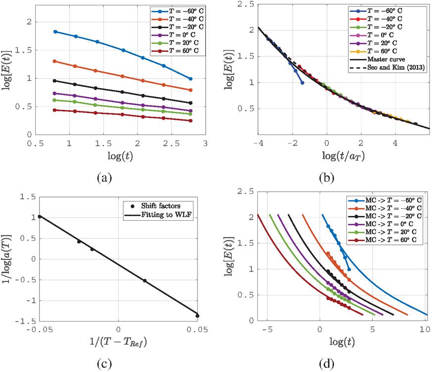
Figure 4 Time-temperature superposition [13]: (a) relaxation modulus at different temperatures, (b) master curve, (c) shift factor parameters, and (d) shifting master curve to other temperatures.
Table 1 WLF constants obtained as discussed in Section 2.3
| WLF Constants | Corresponds to [13] | Corresponds to [14] | Corresponds to [16] |
| 12.53 | 5 | 9.58 | |
| 293.31 | 124.25 | 80.17 |
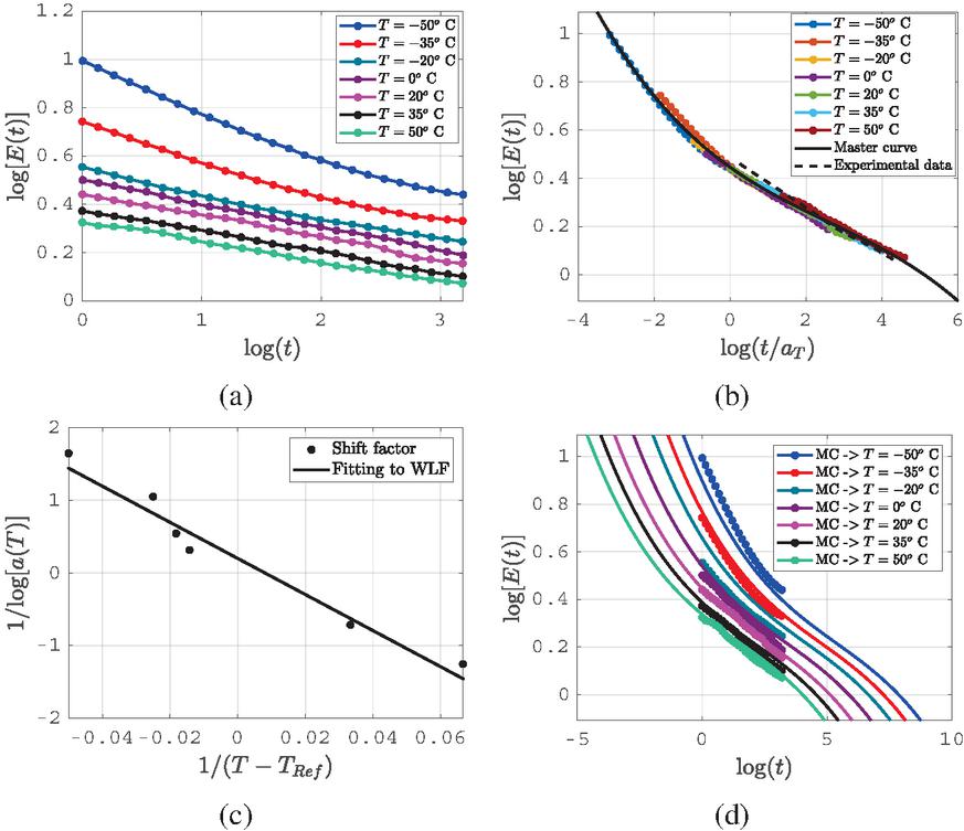
Figure 5 Time-temperature superposition [14]: (a) relaxation modulus at different temperatures, (b) master curve, (c) curve fitting to compute shift factor parameters, and (d) shifting master curve to other temperatures.
The master curves, for relaxation response, are shown in Figures 4 and 5, and for creep response in Figure 6. Experimental VE material response ([13]), in logarithmic scale, is shown in Figure 4(a), where C temperature is taken as the reference temperature. The responses, at temperature higher than C, are thus shifted rightward, and the responses, at temperature lower than C, are shifted leftward (explained in Section 2.2). The shifted curves are then fitted in a cubic polynomial to get the master curve as plotted in Figure 4(b) ([13]). It is seen from Figure 4(b) that the long-term material behaviour is captured successfully by the proposed approach and successfully validated against the experimental results in [13]. The shift factors obtained are further fitted in Equation (6) through a least square approach, as shown in Figure 4(c), to obtain WLF constants. The slope and axis intercept in Figure 4(c) gives WLF parameters at the reference temperature (C) as given in first column of Table 1. The correctness of WLF constants is further verified by shifting the master curve, at reference temperature (C), to other known temperature values as shown in Figure 4(d). The idea is that by shifting the master curve to any other temperature employing WLF constants, the actual experimental curve should overlap with the shifted master curve at that corresponding temperature (shown in Figure 4(d)). It can be observed in Figure 4(d) that the short-time experimental response overlaps with the shifted long-term response thus demonstrating the correctness of obtained WLF constants by Equation (6). There is a slight variation in the shifted curve and experimental curve at C temperature, as seen in Figure 4(d), due to a slight variation in the experiment data itself as seen in Figures 4(a) and 4(b).
A similar master curve computation process is performed (Figure 5(b)) employing another set of relaxation experiment data as given in [14], where C is taken as the reference temperature (Figure 5(a)). The WLF parameters, corresponding to reference temperature C are given in second column of Table 1. It is important to note here that the shifted master curve does not overlap with the experimental response at few temperature values as seen in Figure 5(d). This is happening because, WLF parameters are obtained by approximated straight line fitting (Figure 5(c)), and they may not reproduce all the actual experimental responses.
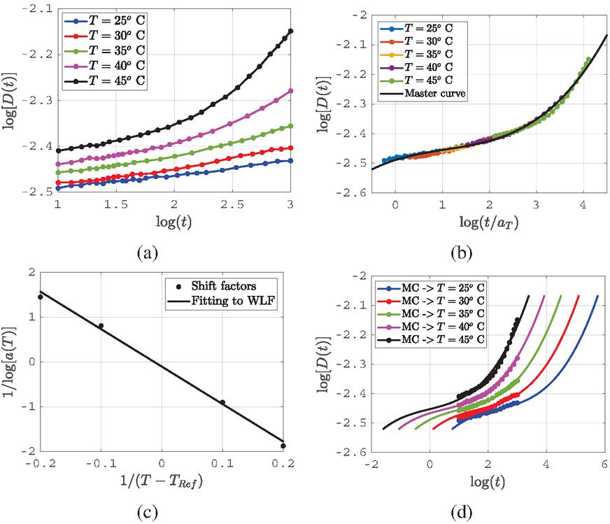
Figure 6 Time-temperature superposition [16]: (a) creep compliance at different temperatures, (b) master curve, (c) shift factor parameters computation, and (d) shifting master curve to other temperatures.
The master curve process is also verified for a creep response behaviour, as given in [14], where the reference temperature is taken as C, corresponding WLF parameters are given in third column of Table 1 and the results are plotted in Figure 6. Figures 4(b), 5(b), and 6(b) thus show long-term behaviour of VE material through the master curve, and Figures 4(d), 5(d), and 6(d) show that an approximate VE material behaviour, at any other temperature, can be obtained by TTS and WLF equation.
The stress update (without accounting hidden damage) with pseudo time concept, as explained in Section 2.4, is validated against data given in [14], and the results are shown in Figures 7(a) and 7(b) for strain rate 0.005498/s and 0.02658/s respectively. The correctness of WLF equation parameters is also verified through stress update with pseudo time. The experimental stress, as given in [14], is available at C (probably hidden damage starts evolving after 0.2 strain). The C is considered as the reference temperature, and the corresponding master curve is obtained, as shown in Figure 5(b), with the corresponding Prony fit data. The VE material stress update, by Equations (13)–(15) and employing all the material properties at C in Equations (13)–(15), is plotted in Figure 7.
The master curve, at C, is then shifted to other temperatures separately (, , and C) computing shift factor by Equation (5) using WLF constants by Figure 5(c). The other temperatures (C) are then treated as reference temperature (separately), and Prony coefficients are then computed at those respective temperatures. The stress at C temperature is then computed by Equation (15), where is computed by Equations (16)–(20) considering constant (temperature not varying with time), and all the plots are shown in Figure 7. It can thus be seen in Figure 7 that the stress at C is well captured up to the damage point (0.2 strain) by TTS application. It is though seen that there is a little variation in beyond which could be due to the fact: (1) small deformation assumption becomes invalid and (2) there is a small variation between actual (from experiment) and computed by WLF equation parameters. The WLF parameters are still approximated by curve fitting (Figure 5(c)), one has to use them carefully while computing the shift factor.
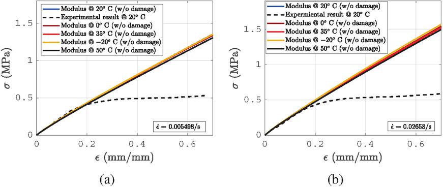
Figure 7 Validation of VE material stress update with pseudo time for data given in [14]: (a) strain rate 0.005498/s, (b) strain rate 0.02568/s.
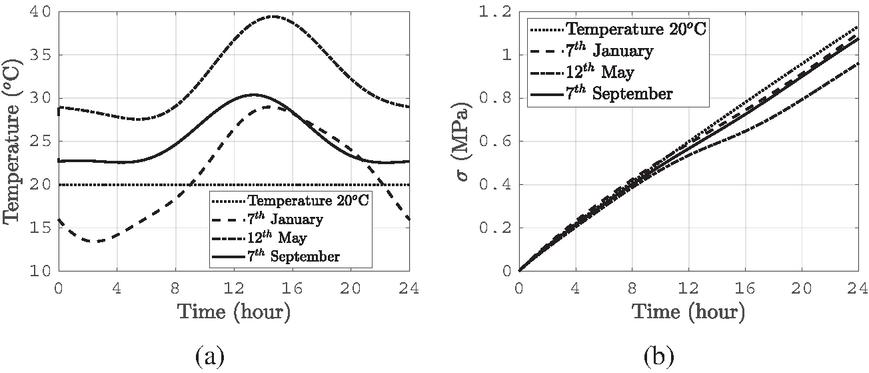
Figure 8 (a) Variation of ambient temperature in a 24 hours day [7], and (b) variation of VE stress corresponding to the ambient temperature.
The variation in ambient temperature, in different seasons, is given in [7], where SRP samples, having hydroxyl terminated poly-butadiene (HTPB), are stored. This temperature variation is fitted in curves to obtain the temperature variation as shown in Figure 8(a). The stress evolutions (computed by Section 3), corresponding to different temperature profiles, are obtained by the properties at reference temperature C ([7]) and plotted in Figure 8(b). It can be observed from Figure 8 that the stress variation changes with the changes in the ambient temperature, i.e., larger value of ambient temperature gives less stress. This happens due to a decrease in the stiffness at higher temperature with reference to the reference temperature (e.g., Figure 5(a)) resulting in lower stress value. This verification case also demonstrates that the response of VE material can be obtained for a temperature variation (by pseudo time concept) knowing the properties at a reference temperature.
4.1 Influence of Thermal Curing Cycle on NEPE Propellant VE Stress Response
A temperature cycle, corresponding to a typical epoxy material (for an illustration purpose), is considered [17], and a constant strain rate is applied to compute VE stress in nitrate ester plasticized polyether (NEPE) propellant. Two thermal cycle profiles, as shown in Figure 9(a), are considered during the curing process, and the corresponding VE stress evolution with time is shown in Figure 9(b). It is seen in Figure 9(b) that (1) VE stress decreases with an increase in temperature, (2) stress curve slope increases with a decrease in temperature, and (3) constant temperature cycle results in an uniform increase of VE stress. This result indicates that VE material stiffness decreases with an increase in temperature and vice versa.
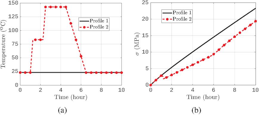
Figure 9 Influence of thermal curing cycle ([17]) on NEPE propellant stress: (a) variation of temperature in a curing cycle, and (b) variation of VE stress at /s [14].
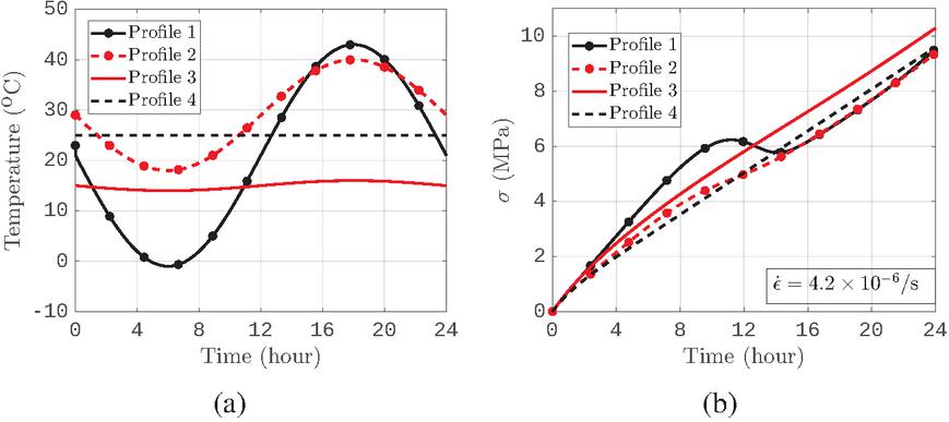
Figure 10 Influence of thermal cycle on asphalt concrete: (a) temperature profiles in a day, and (b) variation of VE stress at /s [18].
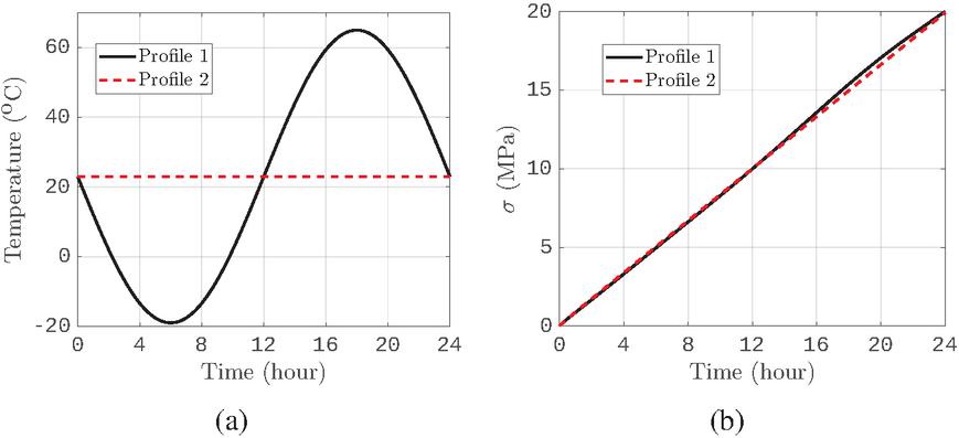
Figure 11 Influence of thermal cycle on HTPB propellant stress: (a) variation of temperature over 24 hours, and (b) variation of VE stress at /s [19].
4.2 Influence of Thermal Cycle on Asphalt Concrete VE Stress Response
Influence of thermal cycle on asphalt concrete stress evolution is now studied. Asphalt concrete is usually exposed to the temperature variation in a day as well as during season changes. The WLF constants, corresponding to NEPE propellant [14] (given in Table 1), are adopted here for asphalt concrete, for illustration purpose, in an absence of experimentally calibrated WLF parameters for asphalt concrete. The temperature profiles, experienced by an asphalt concrete, are shown in Figure 10(a), and the corresponding VE stress evolution is depicted in Figure 10(b). Decrease in the temperature results in an increase in VE stiffness resulting in an increase in the stress, and vice versa, as seen in Figure 10(b), when the profile 1 result is compared with the constant temperature profile result (profile 3). This is expected because of an inverse relation between VE material relaxation modulus and temperature, as illustrated in Figure 5. It is also understood from Figure 10 that asphalt concrete becomes more stiffer, at lower temperature, resulting in lower compliance leading to high stress values. In contrast, high temperature phase of cycle results in decrease in the material stiffness, thus faster stress relaxation.
4.3 Influence of Thermal Cycle on HTPB Propellant Stress Response
The influence of thermal cycle on HTPB propellant stress response is now studied considering a temperature evolution over 24 hours against a constant temperature as shown in Figure 11(a). The WLF constants, for HTPB propellant, are obtained from the shift factors provided in [19], and the corresponding stress response is shown in Figure 11(b). It is again seen that the stress response, under cyclic temperature conditions, deviate from the constant temperature case due to the continuous change in the material relaxation behavior with the temperature.
5 Conclusion
Prony series fit is successfully done for relaxation and creep behaviour of VE material and is validated against the experimental results available in literature. The inter-conversion of VE material behaviour is also successfully validated against the experimental results. A simple process to obtain an appropriate shift factor is proposed, and the same is validated against experimental results. The WLF constants are obtained and verified for known temperature to ensure that these constants can later be used to obtain VE material response at any general temperature. The stress update algorithm is coupled with the shift factor to capture the temperature effect on VE stress update. The incorporation of time–temperature superposition principle, through the shift factor, enables the presented model to account for the temperature-dependent relaxation behavior of viscoelastic materials within the stress computation framework .The effect of temperature cycles on the stress response is demonstrated through different types of VE materials (NEPE propellant, asphalt concrete, and HTPB propellant) subjected to various thermal cycles. The results show that the temperature variation significantly influences the stress evolution due to the changes in material stiffness and relaxation characteristics.
The proposed work will be extended in future coupling VE material stress update with an energy-based damage evolution while capturing fatigue response of VE material.
References
[1] Lakes, R. Viscoelastic materials. Cambridge university press, 2009.
[2] Backman D, Williams J. Advanced materials for aircraft engine applications. Science, 1992, 255:1082–1087.
[3] Patil A, Patel A, Purohit, R. An overview of polymeric materials for automotive applications. Materials Today: Proceedings, 2017, 4:3807–3815.
[4] Maalej Y, El Ghezal M, Doghri I. Micromechanical approach for the behaviour of open cell foams. European Journal Of Computational Mechanics/Revue Européenne De Mécanique Numérique, 2013, 22:198–208.
[5] Payne P. Measurement of properties and function of skin. Clinical Physics And Physiological Measurement, 1992, 12:105.
[6] Bou-Saıd B. A new modeling of human joint lubrication subject to shock loading. European Journal Of Computational Mechanics, 2005, 14:397–420.
[7] Naseem H, Yerra J, Murthy H, Ramakrishna P. Ageing studies on AP/HTPB based composites solid propellants. Energetic Materials Frontiers, 2021, 2:111–124.
[8] Lee D, Cho J. Simplified stochastic temperature model for storage reliability estimation of solid rocket propellants. Journal Of Mechanical Science And Technology, 2023, 37:411–425.
[9] Han L, Tang H. Study on Pavement Mechanics Analysis and Durability Assessment Considering Temperature Effect. European Journal Of Computational Mechanics, 2025, 79–108.
[10] Bradshaw R, Brinson L. A sign control method for fitting and interconverting material functions for linearly viscoelastic solids. Mechanics Of Time-dependent Materials, 1997, 1:85–108.
[11] Rust W. Non-linear finite element analysis in structural mechanics. Springer, 2015.
[12] Jeremic, R. Some Aspects of Time-Temperature Superposition Principle Applied for Predicting Mechanical Properties of Solid Rocket Propellants. Propellants, Explosives, Pyrotechnics, 1999, 24:221–223.
[13] Seo B, Kim J. Estimation of master curves of relaxation modulus and tensile properties for solid propellant. Advanced Materials Research. 2014, 871:247–252.
[14] Han L, Chen X, Xu J, Zhou C, Yu J. Research on the time–temperature–damage superposition principle of NEPE propellant. Mechanics Of Time-Dependent Material, 2015, 19:581–599.
[15] Park S, Schapery R. Methods of interconversion between linear viscoelastic material functions. Part I—A numerical method based on Prony series. International Journal Of Solids And Structures, 1999, 36:1653–1675.
[16] Arzoumanidis A, Silberstein M, Amirkhizi A. Challenges in Mechanics of Time Dependent Materials, Volume 2, Springer, 2018.
[17] Khennache M, Mahieu A, Ragoubi M, Taibi S, Poilâne C, Leblanc N. Physicochemical and mechanical performances of technical flax fibers and biobased composite material: Effects of flax transformation process. Journal Of Renewable Materials, 2019, 7:821–838.
[18] Londono J, Shen R, Waisman H. Temperature-dependent viscoelastic model for asphalt–concrete implemented within a novel nonlocal damage framework. Journal Of Engineering Mechanics, 2020, 146:04019119.
[19] Kim S, Im Y. Experimental study of material behavior of AP-HTPB base composite solid propellant. Journal Of Mechanical Science And Technology, 2019, 33:3355–3361.
Biographies

Priyanka Samal is a research scholar in Department of Aerospace Engineering at Indian Institute of Technology Madras, Chennai, India. She received her M.Tech. degree in Mechanical Engineering from Indian Institute of Technology Bhubaneswar, Odisha, India. Her research areas include modelling Viscoelastic material coupled with damage and healing while considering temperature and ageing effects.

Shantanu S. Mulay is a Professor in Department of Aerospace Engineering at Indian Institute of Technology Madras, Chennai, India. He received his doctorate in Mechanical Engineering from Nanyang Technological University, Singapore (NTU). His current research domains includes constitutive modelling and the fracture studies of composites under fatigue loading, multi-scale modelling of granular materials, multi-physics modelling of soft materials, computation of the macroscopic material constants based on the prescribed motion of the solid and fusion of soil mechanics with the continuum mechanics.
European Journal of Computational Mechanics, Vol. 34_5, 427–448
doi: 10.13052/ejcm2642-2085.3452
© 2026 River Publishers