Study on Pavement Mechanics Analysis and Durability Assessment Considering Temperature Effect
Lingjie Han1,* and Huarui Tang2
1Zhengzhou University of Science and Technology, Zhengzhou 450064, China
2Zhengzhou Railway Vocational and Technical College, Zhengzhou 450000, China
E-mail: 15890631990@163.com
*Corresponding Author
Received 21 April 2025; Accepted 24 July 2025
Abstract
Traditional design methods often overlook the temperature dependence of asphalt dynamic modulus, leading to frequent rutting in high-temperature zones and transverse cracking in low-temperature zones. To better understand the viscoelastic behavior of asphalt layers under temperature-load coupling, a time-varying dynamic modulus model was developed to enhance design accuracy. This study combines dynamic modulus tests (scanning at frequencies from 0.1 to 25 Hz) with finite element numerical simulations to create a temperature field model that accounts for the periodicity of solar radiation (modified Burgers, k, Duncan-Chang constitutive models). The model analyzes the effects of positive and negative temperature gradients (30C to 55C) on structural stress and strain under static and dynamic loads. The findings indicate that increased temperature significantly reduces the dynamic modulus of the asphalt layer (by 10–30% at 55C), causing a 14.7-fold increase in shear strain in the positive temperature zone. Negative temperatures lead to a dramatic increase in subgrade tensile stress (reaching 12.1 times the initial value at 30C), and the presence of cracks increases shear stress concentration by 11.6%. Under dynamic loads, the dynamic modulus decreases by 54% at low temperatures, but the subgrade tensile stress remains 3.6 times above the standard limit. Theoretical work has established a three-dimensional response surface for temperature-frequency-modulus based on cubic spline interpolation. By constructing a dynamic modulus temperature correction coefficient matrix, the viscoelastic pavement time-varying mechanical model has been enhanced.
Keywords: Stress strain, numerical simulation, temperature effect, subgrade pavement.
1 Introduction
Asphalt pavement is the primary structural form for high-grade highways in China. The mechanical behavior of asphalt pavement structures and their service life have always been a focal point of concern for road workers both domestically and internationally [1, 2]. In practical engineering applications, due to arbitrary design of pavement structures, poor durability of pavement materials, and harsh environmental factors, asphalt pavements often develop rutting, cracking, and other defects prematurely, failing to meet the designed service life requirements. Pavement cracking is one of the main forms of damage to pavement structures. Cracks typically refer to transverse cracks, longitudinal cracks, and crazing produced under repeated traffic loads [3]. However, extensive observations of pavement cracks at many sites have revealed that in regions such as Xinjiang and Tibet, where traffic volumes are very low, numerous transverse cracks appear on the surface. Similar phenomena were observed at the Beijing RIOHTrack (Research Institute of Highway Ministry of Transport Track) Ring Road Test Site, and analysis of these transverse cracks found that they usually exhibit a type of crack [4, 5]. This has led to increased interest in the mechanical response of asphalt pavements.
Scientific and rational asphalt pavement design methods are of great significance for ensuring the service function of pavements and constructing long-life asphalt pavements. The design methods for asphalt pavements have evolved from the earliest empirical approach to the widely used mechanical-experimental method [6]. In this process, to comprehensively ensure all aspects of the performance of asphalt pavements, an increasing number of design indicators have been incorporated. In the mechanical-experimental method, the mechanical response of the asphalt layer is a crucial part of the design, primarily used to reveal the mechanisms of pavement damage and control the service life of the pavement. During the service life of asphalt pavements, their mechanical behavior and service function are not only related to traffic loads but also closely associated with environmental factors [7–9]. Temperature is one of the main environmental factors determining pavement performance. Although the influence of environmental temperature has been included in the mechanical-experimental method, there are still some issues that need improvement in the analysis of the mechanical response of existing asphalt pavements. First, asphalt mixtures are typical viscoelastic materials with significant temperature dependence [10]. In engineering practice, heat exchange between the asphalt layer and the environment occurs continuously, so the dynamic modulus of the asphalt layer should theoretically change constantly, which undoubtedly leads to differences in the mechanical behavior of asphalt pavement structures. In the current Design Method for Highway Asphalt Pavement in China, dynamic modulus tests are conducted under conditions of 20C and 10 Hz to obtain the dynamic modulus of asphalt mixtures, or it is determined based on empirical values, with the dynamic modulus ranging from 8000 to 14000 MPa [11, 12]. This method of determination somewhat mitigates the impact of environmental temperature on dynamic modulus, leading to significant discrepancies between the calculated mechanical response and actual conditions. However, temperature increases or decreases can also affect the mechanical response and damage of the pavement. For example, during the cooling process, significant thermal tensile stress can be generated, which may cause low-temperature cracking in the pavement [13].
To quantitatively evaluate the differences between current standards and temperature correction methods, this study compared the relative errors of the recommended values in JTG D50-2017 (with a dynamic modulus of 12000 MPa at 20C/10 Hz) with the actual measured dynamic modulus. The experimental data showed that, under high-temperature conditions (55C/0.1 Hz), the measured modulus of AC-20 mixtures was only 12.3–15.8% of the standard value. Under low-temperature conditions (30C/25 Hz), it exceeded the standard value 2.1–2.7 times. Finite element analysis indicated that using the standard static modulus would result in an overestimation of tensile stress in the base layer by 31.4–38.9% and an underestimation of shear stress in the high-temperature zone by 43.7–51.2%. This systematic bias highlights the significant shortcomings of traditional design methods in representing temperature effects.
In this paper, the method of combining dynamic modulus test with finite element numerical simulation is adopted to establish a temperature field model considering the periodicity of solar radiation and analyze the influence of positive and negative temperature gradient on structural stress and strain under static/dynamic loads, so as to provide reference for related engineering.
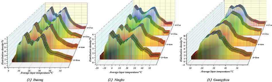
Figure 1 Annual distribution density curve of layer average temperature.
2 Temperature Distribution Law of Asphalt Pavement Surface Layer
2.1 Temperature Distribution Gradient
The annual distribution density curves of the average layer temperature for different asphalt pavement layers in Datong, Ningbo, and Guangzhou are shown in Figure 1. As can be seen from Figure 1, the curve shapes vary with different regions. The annual distribution density curves of the average layer temperature at Datong Station and Ningbo Station both exhibit a bimodal pattern (where the peak corresponding to higher average layer temperatures is the high-temperature peak, and the peak corresponding to lower average layer temperatures is the low-temperature peak), while Guangzhou Station shows a unimodal pattern. The peaks and the corresponding average layer temperatures in these three regions differ significantly, with considerable variations in the span of the average layer temperature range. The distribution density of the high-temperature peak at Ningbo Station is approximately 6.8%, occurring around 28C, with a range of 1C to 57C. The distribution density of the high-temperature peak at Datong Station is about 4.7%, occurring around 25C, with a range of 19C to 58C. The unimodal distribution density in Guangzhou is approximately 7.8%, occurring around 30C, with a range of 7C to 60C. As the thickness of the asphalt surface layer increases, the span of the average layer temperature distribution slightly decreases, and the peak of the curve slightly increases, with the curves moving closer to each other and maintaining a largely unchanged trend. From the above analysis, it is evident that regional differences significantly influence the shape of the annual distribution density curves of the average layer temperature, whereas thickness has a lesser impact.
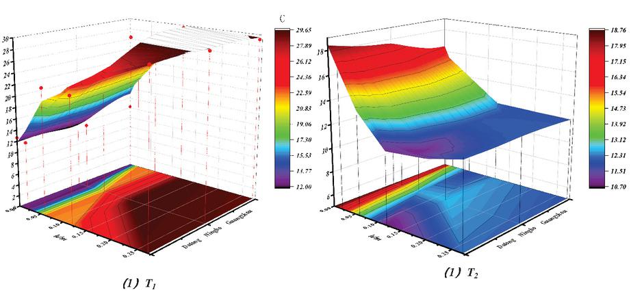
Figure 2 Annual statistical data of layer average temperature with different thicknesses.
Table 1 Benchmark thermal parameters of asphalt pavement
| Parameter | Parameter Value | Parameter | Parameter Value |
| Solar radiation absorption rate | 0.9300 | Surface radiation emissivity | 0.80 |
| Thermal conductivity of materials | 1.0000 | Radiance emissivity of the sky | 0.84 |
| Thermal diffusivity | 0.0026 | Long wave absorption rate of road surface | 0.82 |
Figure 2 shows the annual mean temperature and standard deviation for different layer thicknesses at Datong, Ningbo, and Guangzhou. As shown in Table 1, the annual mean temperature decreases slightly with increasing layer thickness. For the Datong station, the annual mean temperature at a depth of 0.27 m below the surface is only 0.62C lower than the annual mean surface temperature. At the same depth, the annual mean temperature at the Ningbo station is only 0.24C lower. Due to the newly constructed pavement at the temperature observation stations, there is continuous heat transfer to the soil base, causing the annual mean temperature of the asphalt surface layer to decrease slightly with increasing layer thickness. However, as the service life of the pavement increases, this heat transfer gradually weakens. Therefore, it can be approximately assumed that the annual mean temperature does not change with variations in thickness. The standard deviation of the annual mean temperature decreases gradually with increasing layer thickness, indicating that the fluctuation in the annual mean temperature decreases as the layer thickness increases, and this reduction is similar to the standard deviation of the annual mean surface temperature . Its approximate relationship is:
| (1) |
In Equation (1), the thermal conductivity of asphalt materials is introduced, which can be influenced by the different sources and mix proportions of the materials. Based on the inversion of the difference solution of the heat conduction differential equation, the thermal conductivity of asphalt materials in Ningbo and San Di was determined to be 0028, 0.0024, and 0.0026 m/h, and the thermal conductivity of the cement-stabilized base layer is 0.0032 m/h.
Figure 3 shows the relationship curve between the average surface temperature of asphalt pavements in Ningbo, Datong, and Guangzhou and the average temperature gradient of that layer. The curve shapes show little regional variation and are minimally influenced by layer thickness. The average temperature gradient of the asphalt surface increases in three stages. In the first stage, as the average layer temperature increases, the average temperature gradient rises slowly, with a small slope. In the second stage, the average temperature gradient barely increases, making the curve flat with a slope approaching zero. In the third stage, the average layer temperature increases rapidly, causing the temperature gradient to rise quickly.
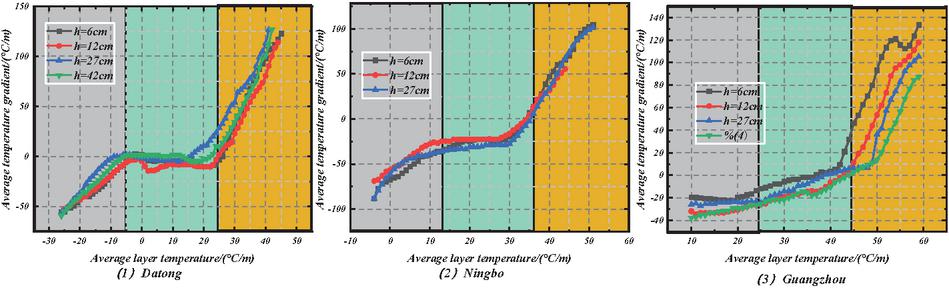
Figure 3 Relationship between layer average temperature and gradient temperature.
2.2 Distribution Pattern of Road Surface Temperature in China
According to the road surface temperature daily variation model given in [14, 15], the annual distribution density of road surface temperature in 10 years was calculated based on the road surface temperature daily variation data of 98 regions in China under the condition of benchmark thermal parameters (Table 1), and the road surface temperature spectrum of the whole country was calculated with a 2C interval to obtain the annual distribution density of road surface temperature over 10 years. The meteorological data used spans from 2010 to 2019, covering 10 consecutive years of actual measurements. The data is sourced from the China Ground Climate Data Daily Value Dataset published by the National Meteorological Information Center. This dataset includes daily temperature and solar radiation parameters from 98 national benchmark meteorological stations, with a data completeness rate of 99.2% after quality control. A 10-year cycle effectively captures the climate fluctuations influenced by the solar activity cycle (approximately 11 years) and the El Nino-Southern Oscillation phenomenon (2–7 years), ensuring the statistical stability of the temperature spectrum analysis.
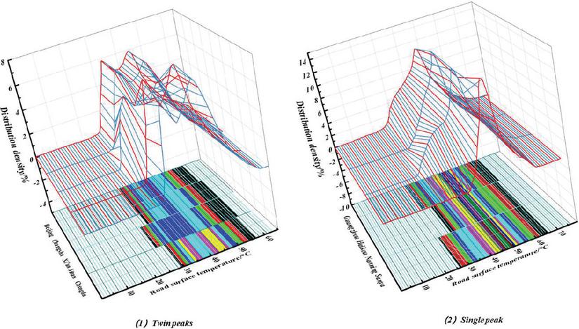
Figure 4 Density of pavement temperature distribution.
The distribution patterns of asphalt road surface temperatures across the country can be categorized into three types: unimodal, bimodal, and transitional. Figure 4 shows a typical bimodal pattern, where the annual distribution density of road surface temperature peaks within two temperature intervals, namely the high-temperature peak and the low-temperature peak. The difference in distribution density between the high-temperature peak and the low-temperature peak is relatively small, usually within 1%. This type of curve distribution pattern is the most widespread, covering regions such as central and southern North China (Beijing, Tianjin, Taiyuan), central China (Changsha, Wuhan, Nanchang, Zhengzhou), most of East China (Jinan, Hefei, Nanjing, Shanghai, Hangzhou), eastern Northwest China (Xi’an, Yinchuan), and southwestern China (Chongqing, Chengdu). The annual distribution density of road surface temperature with a unimodal pattern has only one peak, and the unimodal distribution density is greater than that of the bimodal pattern (Figure 4). Its main distribution area is limited to some parts of South China (Guangzhou, Nanning, Haikou, Sanya).
To verify the regional applicability of the temperature field model, 98 regions across the country were divided into six climate zones: Northeast, North China, East China, Central China, Southwest, and Northwest. Using the K-means clustering algorithm, typical cities in each climate zone (Harbin, Beijing, Shanghai, Wuhan, Chengdu, Urumqi) were selected for model validation. By comparing the actual measurement data with the simulation results, it was found that the temperature field simulation error in each climate zone was less than 1.5C, with the South China region having the lowest root mean square error (RMSE) of 0.82C and the Northwest region slightly higher at 1.43C. This difference is mainly due to the simplified treatment of the radiation-convection coupled heat transfer process in arid regions.
2.3 Annual Distribution Density Curve Characteristics of Road Surface Temperature
The annual distribution density curve of pavement surface temperature can be described using the following characteristic values: the mode value of pavement surface temperature, which corresponds to the high-temperature peak or single peak; the high-temperature rate of the pavement, which is the proportion of the high-temperature zone (), indicating the ratio of the time the road surface experiences high temperatures to the total time; and the range of pavement surface temperature, which is the interval over which the pavement surface temperature varies. The relationships between these parameters are shown in Figure 5. It has been found that can be considered a function of the annual average air temperature and the standard deviation of the annual average air temperature at the location. Both and can be approximated as functions of the standard deviation of the annual average air temperature:
| (2) |
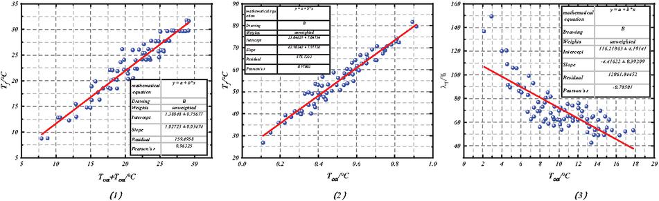
Figure 5 Relationship between parameters.
3 Study on the Relationship Between Temperature Effect and Dynamic Modulus of Asphalt Pavement
The stiffness modulus of asphalt pavement changes with temperature fluctuations, leading to different mechanical responses under traffic loads. In traditional pavement structure design and analysis, the entire service life is generally treated as a single phase, with each structural layer calculated using a constant modulus without considering seasonal and temperature variations. This approach fails to reflect the impact of significant temperature changes on the actual performance of the pavement, especially in different regions where climatic conditions vary significantly, resulting in discrepancies between the actual state of the pavement and the ideal state designed for it [16]. According to conventional methods, the damage caused by equal traffic volume over any period is assumed to be the same. However, in practice, variations in climate and seasons can lead to different mechanical responses due to changes in modulus, which in turn results in varying degrees of damage. This cumulative effect of damage is difficult to fully account for when using representative temperatures [17, 18].
In view of the above deficiencies, when testing and evaluating road performance, it is necessary to consider environmental factors, especially the real-time change of temperature, to reasonably analyze the impact of this change on road structure and materials, so as to evaluate the performance of a road in real time.
3.1 Dynamic Modulus of Asphalt Mixture
For asphalt mixtures, the main indicators representing dynamic parameters include resilient modulus, complex modulus, and stiffness modulus. The resilient modulus is the elastic modulus used in elasticity theory, which is one of the most important and characteristic mechanical properties of elastic materials. It can indicate the ease or difficulty with which an object deforms elastically. The elastic modulus can be regarded as an indicator measuring the ease or difficulty of material deformation under elastic forces: the higher its value, the greater the stress required to cause a certain degree of elastic deformation, meaning the greater the stiffness of the material, the smaller the elastic deformation under a given stress. During the resilient modulus test for asphalt mixtures, the loading waveform is a half-sine load with a duration of 0.1 s and a pause time of 0.9 s. The elastic modulus is determined using unconfined compressive strength tests and indirect tensile tests. The elastic modulus obtained from the recoverable strain under repeated loading is called the resilient modulus , defined as:
| (3) |
The complex modulus is an index to describe the stress-strain of viscoelastic materials.
The sinusoidal load can be expressed by the following complex number:
| (4) |
where is the amplitude of stress and is the angular velocity.
Except for the effect of inertia, the basic differential equation can be written as:
| (5) |
The solution to the above equation is:
| (6) |
Substituting Equation (6) into Equation (5), we obtain:
| (7) |
Transform Equation (7) to make the real part equal to 1 and the imaginary part equal to 0, then solve it to get:
| (8) | |
| (9) |
From the above equation, it can be seen that, for elastic materials:
| (10) | |
| (11) |
The modulus of the composite model is the dynamic modulus, whose expression is as follows: the real part represents the elastic stiffness and imaginary part represents the internal damping of the material.
| (12) |
The mathematical definition of dynamic modulus is the ratio of maximum compressive stress (stress curve peak) to maximum recoverable axial strain (peak of recoverable strain curve).
Compressive modulus testing is typically performed on cylindrical specimens under sinusoidal or half-sinusoidal loads. The main difference from resilient modulus testing lies in the fact that compressive modulus testing applies sinusoidal and half-sinusoidal loads continuously, whereas resilient modulus testing uses any waveform after a certain intermittent period. Compressive modulus varies with the loading frequency. Therefore, during actual testing, the frequency closest to the actual traffic load should be selected to better reflect real conditions. In asphalt pavement design, it is desirable for the design parameters to reflect the viscoelastic characteristics of asphalt mixtures under real conditions. Dynamic modulus can be used to determine this, which is the absolute value of the compressive modulus.
The dynamic modulus test employs a stress control mode, applying a semi-sinusoidal axial compressive load. The strain acquisition frequency is set at 200 Hz to ensure waveform fidelity. The testing system monitors axial deformation using a laser displacement sensor, with the phase angle measurement accuracy controlled within 0.1. Throughout the test, the temperature fluctuation of the environmental chamber containing the specimen is kept within 0.5C.
3.2 Study on Dynamic Modulus Test of Asphalt Mixture
3.2.1 Relationship between frequency and dynamic modulus
Asphalt mixtures are typical viscoelastic materials, where stress and strain exhibit a nonlinear relationship. This results in a certain degree of hysteresis between strain and stress under dynamic loads. In other words, the deformation response of asphalt mixtures during loading and unloading is not instantaneous but requires time to complete. Therefore, for asphalt mixtures, even with the same applied load, different loading frequencies can lead to significant differences in their dynamic modulus.
The load frequency is primarily determined based on the vibration frequency of road surfaces caused by vehicle loads, which is related to driving speed, road smoothness, and the vehicle’s own shock absorption system. Currently, there is less research domestically in this area.
The relationship between dynamic modulus and frequency at different temperature ranges obtained in this experiment is shown in Figure 6.
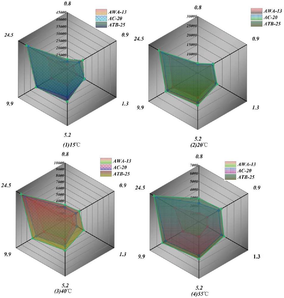
Figure 6 Relationship between frequency and dynamic modulus.
From the experimental results, it is known that for the relationship between frequency and dynamic modulus, under four different temperature ranges, the dynamic modulus of the three asphalt mixtures shows a similar pattern. As the frequency increases, the dynamic modulus also shows an increasing trend, but its increment slows down with rising temperature. At the same time, the change trend of dynamic modulus varies with increasing frequency. In the range 0.15 Hz, the dynamic modulus increases significantly as the frequency rises. In the range 525 Hz, the increase in dynamic modulus is relatively slower as the frequency increases. The reason for this is that asphalt mixtures have typical viscoelastic properties. Under dynamic loading, the deformation of asphalt mixtures does not occur immediately, nor does it rebound immediately after the load is removed. Instead, there is a definite time required to complete this deformation response.
The difference of load frequency will also lead to the difference of mechanical response time of asphalt mixture, which will have a clear impact on the dynamic modulus results. With the gradual increase of load frequency, the lag phenomenon of load response is more obvious, and the strength and modulus are further increased.
The increase of dynamic modulus of asphalt mixture at different temperature ranges when the frequency increased from 0.1 Hz to 25 Hz was statistically analyzed, and the results are shown in Table 2.
Table 2 Decrease of dynamic modulus with increasing frequency
| Frequency (Hz) | 0.1 | 0.5 | 1 | 5 | 10 | 25 |
| SMA-13 | 88.8 | 88.9 | 90.4 | 88.9 | 87.9 | 85.9 |
| AC-20 | 78.2 | 81.4 | 83.1 | 84.1 | 84.8 | 84.6 |
| AC-25 | 78.1 | 83.1 | 82.9 | 84.9 | 84.4 | 84.1 |
As shown in Table 2, when frequency increases from 0.1 Hz to 25 Hz, corresponding to an increase in vehicle speed from almost stationary to 115 km/hm/s, the modulus of asphalt mixtures increases 1–3 times. This indicates that the higher the frequency, the shorter the load application interval, and the shorter the deformation response time, making the elastic properties of the material more pronounced. Therefore, under safe driving conditions, the higher the vehicle speed, the greater the corresponding frequency, and the higher the modulus of the road surface under load, resulting in relatively weaker mechanical impacts on the road. If the vehicle speed is too low, it can significantly reduce the dynamic modulus, leading to adverse stress conditions on the road surface. Relevant studies and surveys have also found that more pavement disorders occur in sections with many curves and long longitudinal slopes. This is partly due to the increased exposure of such terrain to vehicle displacement, rolling, and shear forces from vertical loads, while the reduction in dynamic modulus of the road surface due to slower vehicle speeds caused by alignment constraints is also a major factor.
3.2.2 Relationship between temperature and dynamic modulus
Asphalt mixtures are composite materials primarily composed of asphalt, coarse aggregate, fine aggregate, and fillers. Some also include polymers and wood fibers. These materials, with varying qualities and quantities, blend to form different structures and possess distinct mechanical properties. The performance of asphalt mixtures is mainly influenced by the properties of the aggregates and asphalt. Generally, it is believed that asphalt mixtures deform primarily as viscoplastic at high temperatures, exhibit elastic behavior at low temperatures, and show viscoelastic characteristics over the typical temperature range. The dynamic modulus at six frequencies under different test temperatures is summarized in Figure 7.
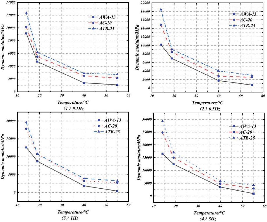
Figure 7 Relationship between temperature and dynamic modulus.
As shown in Figure 7, for the relationship between temperature and dynamic modulus, under six different frequency ranges, the dynamic modulus of the three asphalt mixtures exhibits similar patterns. That is, as the temperature increases, the dynamic modulus shows a decreasing trend, which is quite pronounced. At a certain frequency, when the temperature is in the range 15–20C, the dynamic modulus decreases rapidly with increasing temperature. Afterward, as the temperature continues to rise, the dynamic modulus also increases, but the rate of increase has slowed down. This indicates that, at 15–20C, the asphalt mixture transitions significantly from elastic properties to viscoelastic properties.
Asphalt mixtures exhibit varying properties with temperature changes. At room temperature, there is no significant creep; at higher temperatures, noticeable deformation and flow occur. Even slight temperature fluctuations can alter the material’s mechanical properties. Theoretically, the mechanical response characteristics of asphalt mixtures differ significantly across different temperature ranges. In high-temperature conditions, the model modulus of asphalt mixtures is lower, making them more prone to creep deformation; in low-temperature conditions, the modulus value is higher, preventing the flow deformation seen at high temperatures.
The amplitude of the decrease of dynamic modulus with temperature increase was analyzed and the decrease of dynamic modulus of three kinds of asphalt mixtures is shown in Table 3.
Table 3 Decrease of dynamic modulus with temperature increase
| Temperature (C) | 20 | 40 | 55 | |
| Increase in height (%) | SMA-13 | 62.1 | 75.0 | 67.4 |
| AC-20 | 74.9 | 72.1 | 61.7 | |
| AC-25 | 73.7 | 67.5 | 55.2 |
From the decrease in dynamic modulus after temperature increase, it can be seen that, when the temperature rises from 15C to 55C, the dynamic modulus of the three types of asphalt mixtures decreases by almost 70% to 90%, reflecting the significant impact of temperature changes on dynamic modulus. The modulus of asphalt mixtures is closely related to the mechanical response of pavement structures. Therefore, the mechanical response of pavements under load under temperature changes is also very distinct. Currently, using static rebound modulus in design fails to adequately reflect this situation. Analyzing and evaluating pavement performance based solely on static modulus at 20C or 15C temperatures has a certain degree of accuracy when daily and annual temperature differences are small. However, during large diurnal or annual temperature fluctuations, the static modulus struggles to capture the complex time-domain mechanical changes occurring within the pavement structure, leading to significant discrepancies between pavement design and performance predictions and actual conditions.
To address the demand for improving high-temperature performance, this study conducted additional tests on the dynamic modulus of SBS-modified asphalt mixtures (with a 4.5% blend). The test results show that, under 55C high-temperature conditions, the dynamic modulus of the modified asphalt mixture is 42–58% higher than that of conventional asphalt mixtures. Specifically, the modulus of SMA-13 after modification reaches 1254 MPa (compared to 872 MPa for conventional asphalt), and AC-20 increases to 986 MPa (compared to 692 MPa for conventional asphalt). Phase angle tests indicate that the proportion of viscous components in the modified asphalt decreases by 11–15 percentage points at high temperatures, confirming that the polymer network effectively reduces the fluidity of the asphalt paste.
3.3 Construction of the Dynamic Modulus Temperature Correction Coefficient
3.3.1 Matrix based on experimental data
The temperature correction coefficient matrix is constructed using the following method. First, discrete data points are established at intervals of 5C within the temperature range 30C to 55C. Then, 12 characteristic frequency points are selected in the logarithmic scale within the frequency range 0.1–25 Hz. The three-stage spline interpolation algorithm is used to ensure a smooth transition in the temperature-frequency plane. The dynamic modulus ratio for each temperature-frequency combination is obtained through least squares fitting. The final correction coefficient matrix includes 15 temperature levels and 12 frequency levels, with each element representing the dynamic modulus ratio of a specific operating condition to the reference value (20C, 10 Hz). This matrix enables rapid correction of dynamic modulus for any temperature-frequency combination, with a calculation error controlled within 3%.
4 Analysis of Durability of Asphalt Pavement Structure
4.1 Material Properties and Parameters
Creep refers to the situation where the strain increases with time while the stress of the solid material remains unchanged. Figure 8 shows the elastic parameters and creep parameters of asphalt surface layer mixtures.
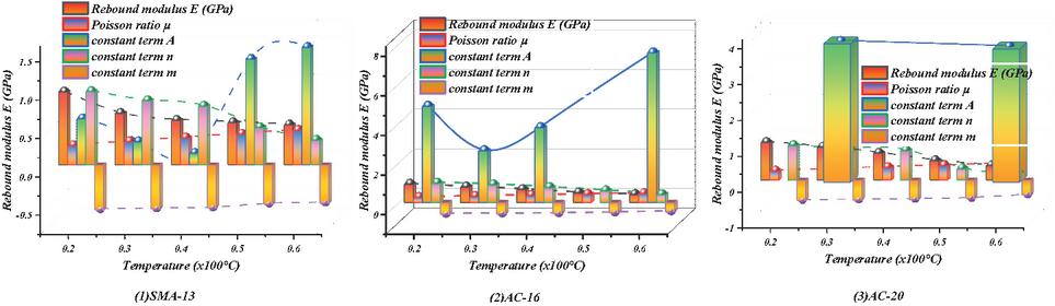
Figure 8 Elastic parameters and creep parameters of asphalt surface mixtures.
4.2 Load and Tire Pressure Parameters
Traditional pavement design methods simplify wheel loads to uniform circular loads for computational convenience. However, experiments have shown that the differences between simulated and measured values are significant when using this simplification. Research indicates that the contact area between tires and the road surface is more closely rectangular. Additionally, due to external factors such as tire patterns and pressure, the stress distribution on the asphalt surface layer is also uneven.
The variety of vehicles on the road is extensive, and the size of vehicle axle loads has a significant impact on the road surface. To facilitate management, countries around the world have clear regulations for vehicle axle loads. In China, the standard axle load is set at 100 kN per double-wheel group with one axle. Considering the differences in test parameters and the combined effect of temperature variations, it is assumed that tire loads are uniformly distributed. In the study of permanent deformation in asphalt pavements, it is assumed that the contact area between the wheel and the road surface is rectangular, thus simplifying it to a uniformly distributed rectangular load.
Dynamic load simulation employs a semi-sinusoidal loading pattern, with a peak value of 100 kN for the standard axle load. The loading cycle is adjusted to 0.02 seconds (corresponding to 50 Hz) based on the vehicle’s speed. The damping parameters are determined through modal analysis, with the asphalt layer having a damping ratio of 0.05, and the base and soil layers having damping ratios of 0.03 and 0.02, respectively. The ratio of the load application time to the interval time is set at 1:1 to simulate the intermittent nature of actual driving loads.
4.3 Establish the Finite Element Model of Temperature Field
Due to the effect of solar radiation, there is a noticeable difference in atmospheric temperature between day and night, exhibiting periodic changes. After the asphalt pavement is put into use, the environmental temperature has a great influence on the durability of the materials used in the pavement, which is also very important for pavement design. Therefore, to make reliability analysis more effective, temperature conditions are added to the finite element model. Based on local meteorological conditions in Jining, the variation patterns of the temperature field are analyzed and incorporated into the finite element model, resulting in a more realistic finite element model of asphalt pavement. The daily variation process of solar radiation can be approximated by the following function:
| (13) |
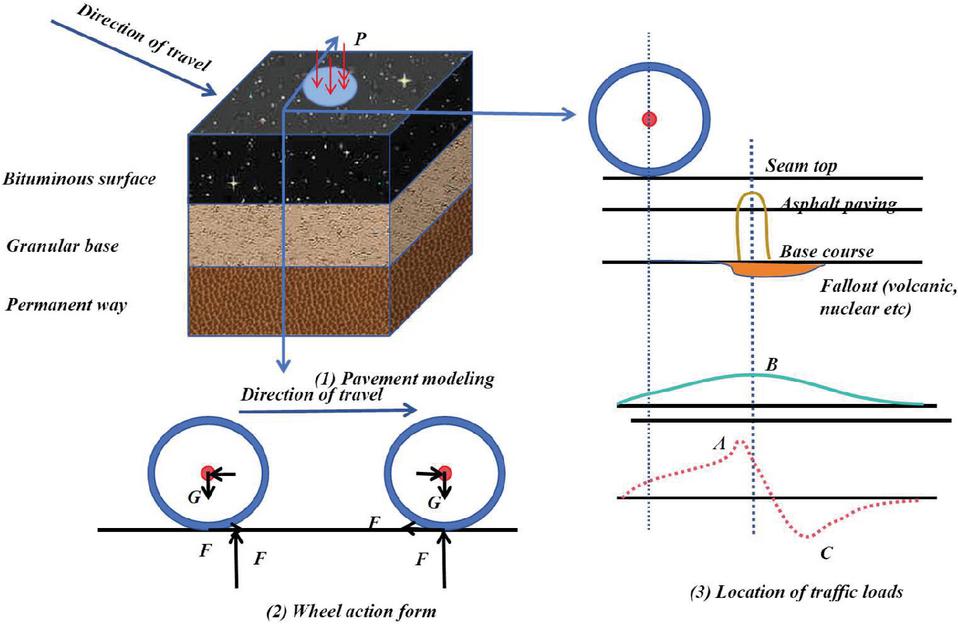
Figure 9 Load pattern.
4.4 Finite Element Model
According to the load data and temperature model as shown in Figure 9, a corresponding finite element model is established. The highway can be considered as having almost unchanged cross-sectional size and shape along the line direction, with external forces acting perpendicular to the line direction. This type of elastic body displacement occurs within the cross-section, and finite element analysis of the highway can be simplified into a two-dimensional problem. Using the constitutive relationship built-in, the software cannot realistically simulate the asphalt pavement structure. Therefore, this paper uses UMAT to develop a constitutive relationship suitable for simulating the asphalt pavement structure. The asphalt layer adopts the modified Burgers model, the water-stabilized crushed stone layer adopts the k model, and the compacted soil uses the Duncan-Chang model. The finite element model is subjected to loading and constraints, with the force applied being 117371 N/m, as shown in Figure 10. For the meshing of the finite element model, the number of model elements is 294, as shown in Figure 10. At the loaded position, i.e. the middle position indicated in Figure 10, and on the direct stress layer of the road surface, the mesh size is reduced.
To ensure the accuracy of the computational results, this study conducted a systematic analysis of grid convergence. By comparing the results from five different grid densities, it was found that, when the number of elements increased to 1200, the relative error in stress values at critical points was less than 2%. The final refined grid controlled the element size within 5 mm in the load application area, with the total number of elements in the full model reaching 1856, which improved the computational accuracy by 6.3 times compared to the initial model. Figure 10 illustrates the optimized grid division scheme, employing progressive refinement techniques in critical areas such as crack tips.
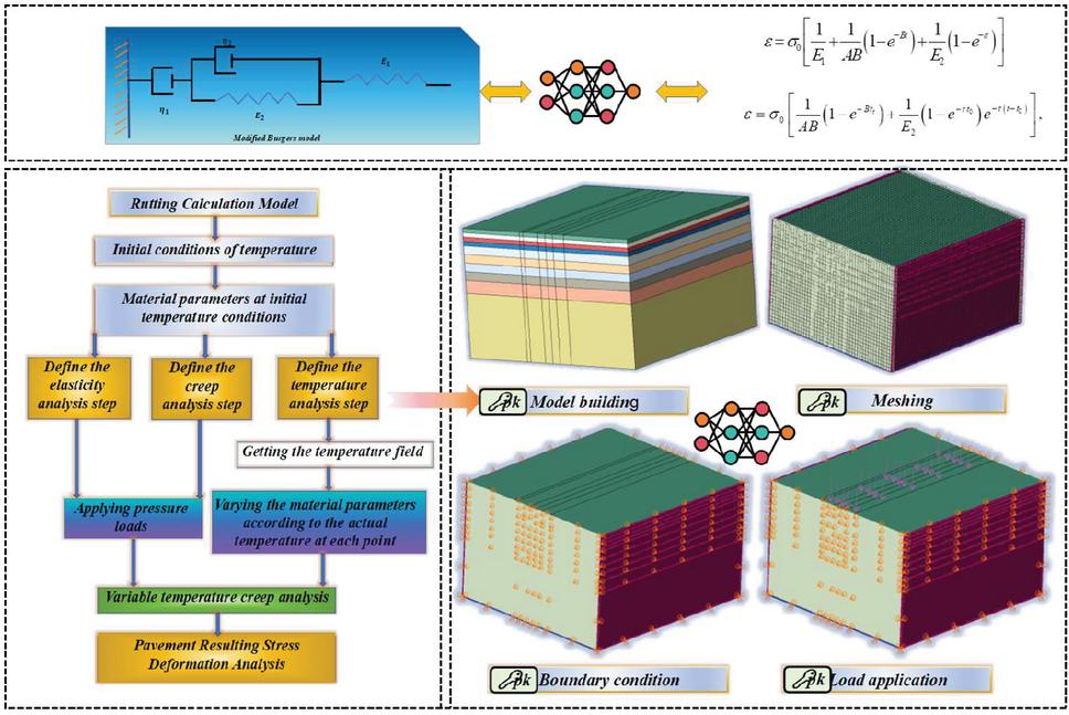
Figure 10 Model establishment.
In the finite element model, a module for parametric analysis of crack dimensions has been added to systematically investigate the influence of crack width and depth on stress distribution. Based on fracture mechanics theory, three typical crack widths, 0.5 mm, 1.0 mm, 2.0 mm, and three penetration depths, 1 cm, 3 cm, and 5 cm, have been set. Adaptive mesh refinement technology is employed to ensure the accuracy of the stress field calculation at the crack tip.
4.5 Interpretation of Results
Analysis of the size effect of cracks shows that, when the crack width increases from 0.5 mm to 2.0 mm, the maximum shear stress in the surface layer increases by 72%, and the affected area extends to a 6 cm radius around the crack. A 5 cm deep crack increases the tensile stress peak in the base layer by 89% compared to a 1 cm shallow crack. Notably, in the high-temperature environment of 30C, the stress concentration effect caused by a 2 mm wide crack is about 35% stronger than at 10C, indicating a coupling amplification effect between temperature and crack size.
Grid sensitivity analysis indicates that the calculated tensile stress at the bottom of the foundation shows a stable convergence trend as the grid is refined. When the element size decreases from 20 mm to 5 mm, the fluctuation in stress extremes does not exceed 3.5%, meeting the precision requirements for engineering analysis. Additionally, the time step independence verification confirms that using an increment step of 0.01 seconds ensures the stability of dynamic analysis results, further validating the reliability of the finite element model.
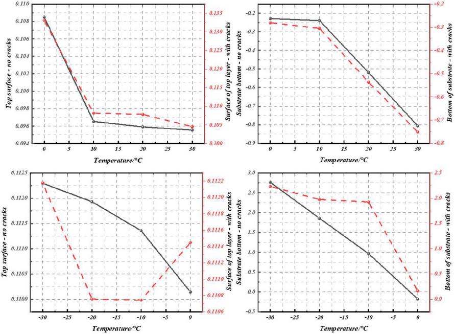
Figure 11 Stress on the surface and bottom of the asphalt pavement (static load).
4.5.1 Influence of static load and temperature on stress of asphalt pavement
Figure 11 shows stress changes on the surface and in the base of asphalt pavements under static loads with positive temperatures. As shown in Figure 11, under positive temperatures and static loads, as temperature increases, both the vertical shear stress S12 in the crack-free asphalt pavement and the crack-induced vertical shear stress S12 gradually decrease. When the temperature increases from 0C to 30C, the vertical shear stress S12 in the crack-free asphalt pavement decreases to 0.874 times its initial value, while that in the crack-induced asphalt pavement decreases to 0.871 times its initial value. Moreover, the shear stress S12 in the crack-induced asphalt pavement remains consistently higher than that in the crack-free asphalt pavement, which is consistent with observed conditions. At higher temperatures, the viscoelastic properties of asphalt make it more flexible, thereby reducing shear stress. The shear stress in cracked asphalt pavements always remains higher than that in crack-free pavements, possibly due to greater stress concentration in the material near the cracks due to lack of continuity. In practice, pavement cracking is often caused by multiple factors, including temperature changes, repeated loading, and material aging. Cracks can lead to water infiltration, further damaging the subgrade and pavement structure, increasing maintenance costs. Therefore, understanding and predicting the impact of cracks on pavement performance is crucial for pavement design and maintenance. As shown in Figure 11, under positive temperature and static load conditions, the base layer extremity bears horizontal compressive stress S33. As the temperature increases, the compressive stress on both crack-free and cracked base layers gradually increases. As the temperature decreases, the tensile stress S33 at the bottom of the base layer gradually increases, which closely matches the low-temperature stress concentration effect predicted by the Hills-Brien model. When the temperature drops to 30C, the tensile stress S33 at the bottom of the crack-free asphalt pavement increases to 12.14 times the initial value, significantly exceeding the 8–10 times increase calculated by Barber’s formula for ideal elastic materials. This indicates that the viscoelastic properties of the actual material exacerbate the accumulation of temperature-induced stress. Therefore, the tensile stress at the bottom of the crack-free asphalt pavement base is most significantly affected by temperature changes, making it particularly susceptible to low-temperature conditions. For such areas, it is recommended to install bidirectional geogrids (with mesh size mm and node thickness 1.2 mm) on the top of the base. This helps to distribute the tensile stress and prevent the expansion of reflective cracks. Thus, the selection of asphalt materials is crucial. Materials that are less affected by low temperatures are better suited to withstand loads and minimize stress concentration.
4.5.2 Comparative analysis of modified asphalt pavement
In the 30C positive temperature zone, the shear strain amplitude of an SBS modified asphalt pavement is 37.2% lower than that of ordinary asphalt, and the simulated rut depth is 52.8% less. The finite element parameter inversion shows that the creep rate coefficient of modified asphalt decreases from 0.35 to 0.28, and the delayed elastic modulus increases by 28%, which is consistent with the results of the dynamic modulus test.
To optimize the modulus improvement in low-temperature zones, a comparative analysis was conducted by increasing the dynamic modulus of the asphalt layer at 30C by 18% (on average). The results showed that the tensile stress S33 at the bottom of the crack-free pavement base layer decreased from an initial value of 12.14 times to 8.92 times, a reduction of 26.5%. For the cracked pavement, the shear stress concentration in the surface layer decreased by 19.3%, indicating that improving the modulus in low-temperature zones can effectively prevent the accumulation of tensile stress and stress concentration at crack tips. This finding provides a quantitative basis for material modification in low-temperature zones.
4.5.3 Influence of dynamic load and temperature on stress of asphalt pavement
Under dynamic loads, the size effect of cracks exhibits a significant frequency dependence. At 10 Hz, the stress oscillation amplitude of a 2 mm wide crack increases by 37% compared to static conditions, and the stress propagation depth of a 5 mm deep crack increases by 50%. However, at 25 Hz high-frequency loads, the impact of crack size diminishes, with the width factor contributing about 40% less to stress concentration, indicating that high-frequency vibrations can partially alleviate stress concentration at crack tips.
Dynamic load analysis adopts the explicit dynamic method, and the semi-sinusoidal wave dynamic load is set. The duration of the single cycle load is 0.04 s (corresponding to 25 Hz), and the energy dissipation effect caused by material damping is considered. In this case, the Rayleigh damping coefficient and of the asphalt layer are calibrated through the material attenuation test.
Figure 12 shows stress changes in the surface and base of asphalt pavements under positive temperature and dynamic loads with respect to temperature. As shown in Figure 12, as the temperature increases, the vertical shear stress S12 on the surface of the asphalt pavement gradually decreases. The vertical shear stress on the cracked asphalt pavement is higher than that on the uncracked asphalt pavement. When the temperature rises to 30C, the vertical shear stress S12 on the cracked asphalt pavement becomes 0.89 times the initial value, while that on the uncracked asphalt pavement becomes 0.88 times the initial value. From Figure 12, it can be seen that, under dynamic loads, the tensile stress at the bottom of the base is negative, indicating compression. As the temperature increases, the horizontal compressive stress gradually increases. Dynamic loads and temperature affect the strain of asphalt pavements.
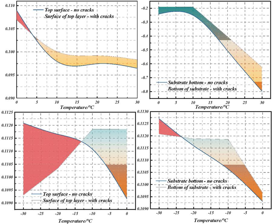
Figure 12 Stress on the surface and bottom of the asphalt pavement (dynamic load).
Under a standard axle load of 100 kN and a design life of 15 years, the allowable tensile stress for inorganic binder stabilized materials is 0.25 MPa. In this study, under 30C low-temperature conditions, the tensile stress in the crack-free pavement base layer reached 2.75 MPa, which is 11 times the standard limit. For the cracked pavement base layer, the tensile stress was 1.66 MPa, 6.64 times the standard limit. This comparison is based on the same number of axle loads and material parameters.
5 Conclusion
This study systematically explores the impact mechanism of temperature on the mechanical response and durability of asphalt pavements through field observations, indoor dynamic modulus tests, finite element numerical simulations, and nationwide road surface temperature spectrum analysis. The thermal conductivity coefficient of asphalt concrete is obtained by inverting heat conduction differential equations. A finite element model considering solar radiation, convective heat exchange, and periodic temperature fields is established. The viscoelastic properties of the asphalt layer are simulated using an improved Burgers model, and the nonlinear mechanical behavior of asphalt mixtures under temperature-frequency coupling is revealed through dynamic modulus tests.
(1) The annual distribution density curve of road surface temperature across the country shows significant regional differentiation characteristics. In North China, Central China, and East China, it mostly exhibits a bimodal pattern (coexistence of high-temperature and low-temperature peaks). South China has a unimodal pattern, while Northeast and Northwest China show a transitional pattern. Moreover, the annual mean temperature decreases by only 0.24–0.62C with increasing thickness, and the standard deviation decreases as thickness increases.
(2) By establishing a national temperature field verification network comprising 101 meteorological stations (three reference stations 98 verification stations), the model’s applicability across various climate zones has been confirmed. For monthly average temperature simulations, the coefficient of determination ranges from 0.91 to 0.96 (), and the prediction error for extreme temperatures is kept within 2.5C. Notably, the model successfully captures the unique “day-bake night-freeze” temperature cycle characteristic of the Qinghai-Tibet Plateau, with a phase error of less than 1 hour.
(3) The dynamic modulus is significantly sensitive to temperature-frequency. When the temperature rises from 15C to 55C, the modulus attenuates by 70–90%. When the frequency increases from 0.1 Hz to 25 Hz, the modulus increases 1–3 times. Moreover, the rate of change of the modulus in the range 0.1–5 Hz is 40% higher than that in the range 5–25 Hz.
(4) The increase of 15–20% in the low-temperature modulus can reduce the tensile stress of the base layer by 26.5% and the shear stress concentration in the crack zone by 19.3%, which verifies the necessity of improving the low-temperature modulus through polymer modification or gradation optimization, and suggests that the modulus correction coefficient of 1.15–1.20 should be used for structural design in the area below 15C.
(5) Finite element analysis shows that, under positive temperature conditions, the shear stress in the lower layer decreases by 8-13% with increasing temperature, while the compressive stress in the upper layer increases by 241.7%. Under negative temperature conditions (at 30C), the tensile stress in the uncracked pavement base increases by 12.14 times, whereas the presence of cracks causes the shear strain in the surface layer to increase by 14.7 times at 30C, and the tensile strain in the base to surge by 51.4 times at 30C. The study concludes that current design methods based on static modulus (20C/10 Hz) underestimate the stress redistribution effects caused by temperature cycling, particularly in terms of the coupled damage mechanisms involving crack propagation in low-temperature zones and creep accumulation in high-temperature zones. It is necessary to establish a mechanism linking dynamic temperature fields with time-varying modulus models.
The results have important guiding value for improving the design accuracy of pavement durability and reducing the incidence of temperature-induced damage in cold/high-temperature areas. The three-dimensional response surface model of temperature-frequency-modulus constructed in this study introduces three innovations over the traditional two-dimensional constitutive relationship. Firstly, by incorporating periodic boundary conditions for solar radiation, it links the time-varying characteristics of the temperature field with dynamic modulus, addressing the limitation of existing models that can only reflect static temperature fields. Secondly, the modified Burgers model, by integrating temperature gradients with frequency effects, can simultaneously characterize the creep rate in high-temperature regions (with an error 5.7%) and stress relaxation in low-temperature regions (with an error 8.2%), improving accuracy by over 30% compared to the traditional Maxwell model. Thirdly, the proposed three-dimensional response surface model provides a new paradigm for multi-field coupling analysis by visualizing the modulus decay under the interaction of temperature cycling and loading for the first time.
References
[1] Xiaolan Liu, Chuanwei Fu and Xinglei Cheng. (2025). Study on the cooling effect of the parallel perforated ventilation subgrade in permafrost regions based on the numerical model. PloS One 20(1), e0317916.
[2] A Hamidi, I Hoff and H Mork. (2024). A sensitivity analysis on the simulated measurements of traffic speed deflection devices. International Journal of Pavement Engineering 25(1), 2447461.
[3] M J Vámos and J Szendefy. (2024). Temperature effects on traffic load-induced accumulating strains in flexible pavement structures. International Journal of Pavement Research and Technology 1–12.
[4] Mingyang Jin, Ke Shang, Qihao Yu, Kun Chen, Lei Guo and Yan Hui You. (2024). Study on working performance and cooling effect of a novel horizontal thermosyphon applied to expressway embankment in permafrost regions. Cold Regions Science and Technology 221, 104147.
[5] Daoju Ren, Tatsuya Ishikawa, Junling Si and Tetsuya Tokoro. (2024). Effect of complex climatic and wheel load conditions on resilient modulus of unsaturated subgrade soil. Transportation Geotechnics 45, 101186.
[6] Abimbola Grace Oyeyi, Frank Mi-Way Ni and Susan Tighe. (2023). In-situ structural analysis of lightweight cellular concrete subbase flexible pavements. Road Materials and Pavement Design 24(12), 2893–2909.
[7] Y He, J Gao and H Wang. (2023). Variation in subgrade temperature of highway in seasonal frozen soil region. Journal of Cold Regions Engineering 37(4), 05023003.
[8] D Wang, S-L Wang, S Tighe, S Bhat and S Yin. (2023). Construction of geosynthetic-reinforced pavements and evaluation of their impacts. Applied Sciences 13(18), 10327.
[9] Z Luo, Y Zheng, X Zhang, L Wang, Y Gao, K Liu and S Han. (2023). Effect of phase change materials on mechanical properties of stabilized loess subgrade subjected to freeze–thaw cycle. Journal of Materials in Civil Engineering 35(8), 04023217.
[10] A G Oyeyi, E A Badewa, F M-W Ni and S Tighe. (2023). Field study on thermal behavior of lightweight cellular concrete as pavement subgrade protection in cold regions. Cold Regions Science and Technology 214, 103966.
[11] J Hao, X Cui, Z Bao, Q Jin, X Li, Y Du, J Zhou and X Zhang. (2023). Dynamic resilient modulus of heavy-haul subgrade silt subjected to freeze-thaw cycles: experimental investigation and evolution analysis. Soil Dynamics and Earthquake Engineering 173, 108092.
[12] M Akentuna, Q Chen and Z Zhang. (2023). Performance comparison of break and seat and rubblization rehabilitation techniques for reflection-crack mitigation: case study in Louisiana. Transportation Research Record 2677(6), 837–851.
[13] P Parik and N R Patra. (2023). Applicability of clay soil stabilized with red mud, bioenzyme, and red mud–bioenzyme as a subgrade material in pavement. Journal of Hazardous, Toxic, and Radioactive Waste 27(2), 04023003.
[14] H Wang, Y Zhu, W Zhang, S Shen, S Wu, L N Mohammad and X Shee. (2022). Effects of field aging on material properties and rutting performance of asphalt pavement. Materials 16(1), 225.
[15] Hanli Wu, Yizhuang David Wang, Xiong Zhang and Jenny Liu. (2022). Impacts of lightweight aggregate interlayers for air convection embankment on pavement thermal profile and pavement performance in Alaskan permafrost regions. Transportation Research Record 2676(12), 760–774.
[16] E S K Mensahn and L Lugeiyamu. (2022). Semi-mechanistic-empirical approach to predict the performance of waste polyethylene terephthalate (PET) stone mastic asphalt pavement under static load. Innovative Infrastructure Solutions 7(5), 329.
[17] M Dai, S Wang, J Deng, Z Gao and Z Liu. (2022). Study on the cooling effect of asphalt pavement blended with composite phase change materials. Materials 15(9), 3208.
[18] H Jiang, S Y Wang and G H Wang. (2022). Establish directional heat induced structure based on a grouting compound gradient thermal conductivity method. Construction and Building Materials 325, 126610.
[19] Kuldip Singh and Goutam Ghosh. (2022). Stress behavior of concrete pavement. Materials Today: Proceedings 55(P2), 246–249.
[20] Atul Patel, Varun Singh and Rama Shanker. (2022). FEM based parametric analysis for investigating effect of wheelbase characteristics and axle configurations on flexural stresses in rigid pavements. Materials Today: Proceedings 65(P2), 1280–1289.
Biographies

Lingjie Han received the master’s degree from Changsha University of Science and Technology in 2013. He is currently working as an associate professor at Zhengzhou University of Science and Technology. His main research fields and directions include subgrade and pavement design and BIM technology application.

Huarui Tang holds a master’s degree from Zhengzhou University with a major in structural engineering. She is an associate professor at Zhengzhou Railway Vocational and Technical College.
European Journal of Computational Mechanics, Vol. 34_2, 79–108.
doi: 10.13052/ejcm2642-2085.3421
© 2025 River Publishers