Crack Analysis Method Based on a Combination of Meshfree Method and Continuous Damage Mechanics

Hyo-Song Kim¹, Jang-Chol Hwang¹, Kumchol Yun¹, Jun-Hyok Ri² and Chi-Myong Kim³

¹Faculty of Mechanics, Kim Il Sung University, Pyongyang, DPR Korea
²Institute of Mechanics, State Academy of Sciences, Pyongyang, DPR Korea
³Faculty of Civil Engineering, Pyongyang University of Transport, Pyongyang, DPR Korea
E-mail: hs.kim1225@ryongnamsan.edu.kp; cioc5@ryongnamsan.edu.kp; kc.yun0705@ryongnamsan.edu.kp; cioc6@ryongnamsan.edu.kp; cioc7@ryongnamsan.edu.kp
*Corresponding Author

Received 05 August 2025; Accepted 08 April 2026

Abstract

In this paper, the application method of continuum damage mechanics in the framework of the element-free method is established. The method of mapping the damage parameters used in continuous damage mechanics (CDM) to the nodes and damping of the element stiffness matrix by the damage parameters are discussed. Since the method of constructing the global stiffness matrix from the element stiffness matrix in the element-free Galerkin method, one of the typical meshfree methods, is different from the finite element method, the continuous damage mechanical model as in the finite element method cannot be applied. To predict the damage initiation and crack propagation directions, the maximum principal stress criterion is used and CDM model is used to predict the damage evolution process under quasi-static loading. The calculated results are compared with several experimental results and show good agreement.

Keywords: Element-free Galerkin (EFG) method, continuous damage mechanics (CDM) model, damage initiation, damage evolution process.

1 Introduction

One of the most popular numerical methods in computational solid mechanics is the traditional finite element method and this is the oldest numerical method for crack modeling. Here, cracks are confined to propagate along interelement edges and it requires remeshing after crack growth at each load step. This disadvantage leads to overestimation of the fracture energy when the actual crack path is not along element interfaces.

The extended finite element method (XFEM) does not require remeshing [1–3, 37]. The dependence of crack modelling on remeshing is generally overcame by adding enrichment functions in the polynomial approximation space. There is no constraint to limit the crack extension path such that cracks are only allowed to develop along interelement edges, and cracks may pass through elements in XFEM. However, XFEM has some disadvantages. The computational approach is complex and requires high computational cost. in multiple crack problems [4], it needs an accurate description of the crack propagation process computed by complicated techniques. The embedded discontinuity model [5–9] does not require a crack surface representation, but these methods require the crack to propagate one element at a time. As a result, this method is very sensitive to the quality of the mesh.

Recently, the phase field method (PFM) [37] has become a popular method for simulating arbitrary crack growth. PFM introduces the regularized representation of sharp crack topology. PFM assumes the crack is not sharp and the crack surface can be diffused over the entire domain by a crack density function. PFM does not require additional tracking algorithms for the continuity and mesh independence of the crack path, and it can successfully simulate crack branching and crack coalescence as well as crack propagation.

PFM has the disadvantage that the simulation results are highly dependent on regularization parameters. In [38], an alternative to combining PFM with continuous damage mechanics (CDM) models is proposed to remove dependence on the regularization parameter. Several mesh-based numerical methods have been combined with tracking algorithms [10–13] to obtain accurate crack propagation paths. Since the results of crack analysis are highly dependent on the tracking algorithm, the study of several numerical methods such as embedded discontinuity models and XFEM are closely related with the study of tracking algorithms.

Currently, the level set method, scalar field method, and explicit tracking algorithms are widely used as tracking algorithms. In the level set method, the crack surface is generally represented by two orthogonal level set functions, which is the most widely used method in failure simulation [14]. The level-set method has been successfully simulated in the fracture problem by combining it with XFEM or meshfree methods, and its research is ongoing [15–19, 38]. In the scalar field method (also called global tracking algorithm) developed by Oliver [11, 20], a scalar field is added to the entire domain and the iso-surface of this scalar field is used to describe the fracture surface. To obtain the scalar values on all nodes at each loading step, the Laplace equation with anisotropic conductivity must be solved. Since the crack path can be determined only after obtaining scalar field information for the entire domain at each loading step, a higher computational cost is required for crack path tracking.

The explicit tracking algorithm, which does not depend on mesh size, has also been widely studied. The method can avoid the influence of mesh size on the crack surface but is difficult to use in commercial finite element analysis software due to a series of techniques required for the generation of crack mesh. Meshfree methods [21–24, 27], such as mesh distortion, volume locking, and mesh dependency presented in mesh-based methods, can be resolved and do not require remeshing and accurate representation of the crack geometry. Many meshfree methods, such as element-free Galerkin (EFG), meshless local Petrov-Galerkin (MLPG), and reproducing kernel particle (RKPM), are widely used in failure analysis.

The cracking particle method based on the EFG method proposed by Rabczuk [25] represents a continuous crack curve by unconnected linear segments. The method describes the crack path by modeling discrete cracks. Crack path consists of a set of contiguous cracking particles. The cracking particle method is simple, compared to the previous methods, because it simulates the crack growth process by simply adding cracked particles.

There are some disadvantages to these element-free methods. First, some techniques are required for the treatment of boundary conditions, since the shape functions used in meshfree methods typically do not have the Kronecker delta property. Also, to model discontinuities such as cracks, meshfree methods have to modify the influence domain of some nodes or add some terms to the basis function to construct a new basis function [26]. Ge nerally, meshfree methods need more computational time than FEM. As the crack tip position changes at each loading step during crack propagation, it takes computational time to re-evaluate the influence domain of nodes near the crack tip and to repeat searching nodes included in the influence domain. To avoid inherent difficulties in the meshfree methods, it has been successfully combined with FEM. These combined methods have advantages over both the meshfree and the FE methods [28–33].

In this paper, a fracture analysis model combines the EFG method with CDM. CDM is widely applied to fracture analysis problems in the framework of the finite element method. This method can obtain representation of the crack surface and the crack propagation curve without using any tracking algorithm, and the crack geometry is naturally obtained by the calculation results. To verify the effectiveness and accuracy of the proposed method, the results of calculations are compared with experimental results.

2 Element-free Galerkin Method and Continuum Damage Mechanics Model

2.1 Element-free Galerkin Method

In the EFG method, the displacement function $u(x)$, which is the main unknown function, is approximated by the polynomial basis function $p(x)$:

$$u^h(\mathit{x})=\sum _{j=1}^m{p}_j(\mathit{x})a_j(\mathit{x})={\mathit{p}}^T(\mathit{x})\mathit{a}(\mathit{x})$$

(1)

where $u^h(\mathit{x})$ is approximated displacement, $\mathit{p}(\mathit{x})$ is polynomial basis function, and unknown coefficient vector $\mathit{a}(\mathit{x})$ is function of the spatial coordinates ${\mathit{x}}^T=[x,y]$. $m$ is the number of terms in the basis. For example, if the basis function is given by

$${\mathit{P}}^T(\mathit{x})=\{1xy\}$$

(2)

then $m$ is 3.

In the moving least squares (MLS) approximation, the basis functions generally use linear or quadratic functions.

The unknown coefficient $\mathit{a}(\mathit{x})=[a_1(\mathit{x}),a_2(\mathit{x}),\mathrm{\dots },a_i(\mathit{x}),\mathrm{\dots },a_m(\mathit{x})]$ is determined by minimizing the weighted residual square function given by

$$J=\sum _{i=1}^{n}W(\mathit{x}-{\mathit{x}}_i){[{\mathit{p}}^T\left({\mathit{x}}_i\right)\mathit{a}(\mathit{x})-{\mathit{u}}_i]}^2$$

(3)

where $n$ is total number of nodes, $W(\mathit{x}-{\mathit{x}}_i)$ is weight function, ${\mathit{u}}_i$ is nodal value at $\mathit{x}={\mathit{x}}_i$. There are several weight functions, but we used cubic spline curves:

$$\frac{\partial J}{\partial \mathit{a}}=0$$

(4)

to obtain

$$\mathit{A}(\mathit{x})\mathit{a}(\mathit{x})=\mathit{B}(\mathit{x}){\mathit{U}}_s$$

(5)

where

$$\mathit{A}(\mathit{x})=\sum _{i=1}^{n}W(\mathit{x}-{\mathit{x}}_i)\mathit{p}({\mathit{x}}_i){\mathit{p}}^T({\mathit{x}}_i)$$	(6)
$$\mathit{B}(\mathit{x})=[W(\mathit{x}-{\mathit{x}}_1)\mathit{p}({\mathit{x}}_1)W(\mathbf{x}-{\mathbf{x}}_2)\mathit{p}({\mathit{x}}_2)\mathrm{\dots }W(\mathbf{x}-{\mathbf{x}}_n)\mathit{p}({\mathit{x}}_n)]$$	(7)
$${\mathit{U}}_s={\{u_1{u}_2\mathrm{\dots }{u}_n\}}^T$$	(8)

From Equation (5) the following expression is obtained

$$\mathit{a}(\mathit{x})={\mathit{A}}^{-1}(\mathit{x})\mathit{B}(\mathit{x}){\mathit{U}}_S$$

(9)

Substituting Equation (9) into Equation (1)

$$u^h(\mathit{x})=\sum _{i=1}^n{\phi }_i(\mathit{x})u_i={\mathrm{\Phi }}^T(\mathit{x}){\mathit{U}}_S$$

(10)

where

${\phi }_i(\mathit{x})$	$={\displaystyle \sum _{j=1}^m}{p}_j(\mathit{x}){({\mathit{A}}^{-1}(\mathit{x})\mathit{B}(\mathit{x}))}_{ji}={\mathit{p}}^T(\mathit{x}){({\mathit{A}}^{-1}\mathit{B})}_i$	(11)
${\mathrm{\Phi }}^T(\mathit{x})$	$=\{{\phi }_1(\mathit{x}){\phi }_2(\mathit{x})\mathrm{\cdots }{\phi }_n(\mathit{x})\}={\mathit{p}}^T(\mathit{x}){\mathit{A}}^{-1}(\mathit{x})\mathit{B}(\mathit{x})$	(12)

The function $\mathrm{\Phi }(\mathit{x})$ is called the MLS shape function. Using the MLS shape function, the nodal stiffness matrix can be obtained

$$K_{ij}={\int }_{\mathrm{\Omega }}{B}_i^{T}C{B}_j\mathit{d}\mathrm{\Omega }$$

(13)

then

$$B_i=\left[\begin{array}{cc}\partial /\partial x& 0\\ 0& \partial /\partial y\\ \partial /\partial y& \partial /\partial x\end{array}\right]\left[\begin{array}{cc}{\phi }_i& 0\\ 0& {\phi }_i\end{array}\right]=\mathit{L}{\mathit{\phi }}_i$$

(14)

where $\mathit{L}$ is differential operator matrix, ${\mathit{\phi }}_i$ is a shape function matrix constructed by a shaped function ${\phi }_i$ and $\mathit{C}$ is elastic matrix, $\mathrm{\Omega }$ is problem domain:

$$\mathit{C}=\frac{E}{1-v^2}\left[\begin{array}{ccc}1& v& 0\\ v& 1& 0\\ 0& 0& (1-v)/2\end{array}\right]\text{(plane stress)}$$

(15)

In the plane strain state, we have

$$\mathit{C}=\frac{E(1-v)}{(1+v)(1-2v)}\left[\begin{array}{ccc}1& \frac{v}{1-v}& 0\\ \frac{v}{1-v}& 1& 0\\ 0& 0& \frac{1-2v}{2(1-v)}\end{array}\right]\text{(plane strain)}$$

(16)

where $E$ and $v$ are Young’s modulus and Poisson’s ratio, respectively. The global stiffness matrix $\mathit{K}$ is obtained by assembling the nodal stiffness matrix $K_{ij}$ as follows

$$\mathit{K}=\left[\begin{array}{cccc}{\mathit{K}}_{11}& {\mathit{K}}_{12}& \mathrm{\cdots }& {\mathit{K}}_{1\mathrm{n}}\\ {\mathit{K}}_{21}^{11}& {\mathit{K}}_{22}^{12}& \mathrm{\cdots }& {\mathit{K}}_{2\mathrm{n}}\\ \mathrm{⋮}& \mathrm{⋮}& \mathrm{\ddots }& \mathrm{⋮}\\ {\mathit{K}}_{\mathrm{n1}}& {\mathit{K}}_{\mathrm{n2}}& \mathrm{\cdots }& {\mathit{K}}_{\mathrm{nn}}\end{array}\right]$$

(17)

Hence, the global system equation is

$$\mathit{K}{\mathit{U}}_s=\mathit{F}$$

(18)

Equation (18) is a set of $n$ algebraic equation, and we solve this system to obtain ${\mathit{U}}_s$ and substitute it into Equation (10) to obtain the nodal displacement.

2.2 Continuum Damage Mechanics Model

In this paper, the EFG method is combined with an advanced continuum damage mechanics model proposed in Yun [34]. Since this CDM model takes into account the propagation direction of discrete cracks, it is possible to model the crack growth process more accurately than the conventional continuum damage mechanics model. In this paper, we have only considered isotropic materials in two-dimensional space for simplicity of the problem without loss of generality.

Generally, the CDM approach is used in the framework of the finite element method. The results of the calculations, including stress, strain, and damage, are values in the element. However, the situation is different for the meshfree methods. Note that although the CDM model is described in the framework of the FEM, all the computational results are values at the nodal points. The effective stress is expressed as

$$\mathit{\sigma }=(1-D)\mathit{C}\mathit{\epsilon }$$

(19)

where $\mathit{\sigma }$ and $\mathit{\epsilon }$ are the effective stress tensor and strain tensor, respectively, $D$ is the damage variable, and $C$ is the elastic matrix. It is assumed that the damage variable $D$ is followed by an exponential softening law

$$D(r)=1-\frac{1}{r}\exp \{-2H_S(r-1)\}$$

(20)

where $H_s$ is the softening parameter and $r$ is the elastic domain threshold. The $r$ has a value of 1 when the material is undamaged and increases as the damage evolves. The softening parameter $H_s$ is defined by using the characteristic length of the element as

$$H_s=\frac{l_e}{l_{mat}-l_e}$$

(21)

where $l_{\mathrm{mat}}$ is the material characteristic length depending on the material properties and defined as

$$l_{mat}=\frac{2E{G}_c}{{\sigma }_f^2}$$

(22)

where $G_c$ is the energy release rate of material, ${\sigma }_f$ is the uniaxial tension strength, and $l_e$ is characteristic length of element. The $r$ at the time step $t+\mathrm{\Delta }t$ is expressed as

$r_{t+\mathrm{\Delta }t}$	$=\max \{1,\underset{\tau =\overline{0,t}}{\max }\{{\phi }_{\tau }\}\}$	(23a)
$r_{t+\mathrm{\Delta }t}$	$=\max \{1,\underset{\tau =\overline{0,t}}{\max }\left\{{\phi }_{\tau }\right\}\}$	(23b)

where ${\varphi }_{\tau }$ is the loading function at time step $\tau$. Loading function $\varphi$ is defined as the normalized equivalent $s$ tress

$$\varphi =\frac{⟨\tilde{\sigma }⟩}{{\sigma }_f}$$

(24)

where $\tilde{\sigma }$ is the equivalent stress and $⟨\cdot ⟩$ is the McCauley operator.

2.3 How to Define the Characteristic Length of Element in the Meshfree Methods

In FEM, the characteristic length of the element is defined as $l_e=\sqrt{A}$ or $l_e=1.52\sqrt{A}$, depending on whether its a square element or triangular element [34], where $A$ is an element area. In the finite element method, the element area can be considered as the element integral area used in numerical integration. In this sense, it is reasonable to consider the characteristic length of $l_e=\sqrt{A_q}$ in the EFG method, where $A_q$ is the area of a background integral cell. We consider the background integration cell as a rectangular region and calculate it.

In MLPG (meshfree local Petrov-Galerkin method), the characteristic length is set according to the type of integration domain because the integral domain is defined for each node distributed in the problem domain. We will only discuss the EFG method. This is because the method of constructing the element stiffness matrix and the global stiffness matrix in the meshfree local Petrov-Galerkin method is similar to that in the finite element method. In other words, the finite element method constructs the global stiffness matrix by assembling the element stiffness matrix corresponding to the element in the global stiffness matrix, and the meshfree local Petrov-Galerkin method constructs the global stiffness matrix by assembling the nodal stiffness matrices corresponding to each node in the the global stiffness matrix in a row-by-row. However, in the EFG method, the global stiffness matrix is constructed from the nodal stiffness matrix computed at the Gaussian points of each background integral cell. This will be discussed in detail in the next section.

3 Numerical Implementation

In the EFG method, the global stiffness matrix is

$$K=\left[\begin{array}{cccc}{K}_{11}& K_{12}& \mathrm{\cdots }& K_{1N}\\ K_{21}& K_{22}& \mathrm{\cdots }& K_{2N}\\ \mathrm{⋮}& \mathrm{⋮}& \mathrm{\ddots }& \mathrm{⋮}\\ K_{N1}& K_{N2}& \mathrm{\cdots }& K_{NN}\end{array}\right]$$

(25)

where $K_{ij}(i\in 1,\mathrm{\dots },N,j\in 1,\mathrm{\dots },N)$ is nodal stiffness matrix and $N/2$ is the total number of nodes. At the first load step, each node is assigned a damage value ranging from 0 to 1

$$K_J=\left[\begin{array}{cccc}{K}_{11}& K_{12}& \mathrm{\cdots }& K_{1n}\\ K_{21}& K_{22}& \mathrm{\cdots }& K_{2n}\\ \mathrm{⋮}& \mathrm{⋮}& \mathrm{\ddots }& \mathrm{⋮}\\ K_{n1}& K_{n2}& \mathrm{\cdots }& K_{nn}\end{array}\right]$$

(26)

If the stiffness matrix of the $J$-th node is found using Equation (26), in the CDM model, the stiffness matrix considering the material property degradation is

$$K_J^{\prime }=(1-d_J)K_J$$

(27)

In Equation (26), $n$ is the number of nodes in the influence domain of the $J$-th node, and in Equation (27), $d_J$ is the damage value of the $J$-th node. The damage variable $D=[d_1{d}_2\mathrm{\dots }{d}_N]$ is calculated at each load step, and the damage values at each node are taken as the maximum value compared to the damage values at the previous load step. Therefore, if the global stiffness matrix is reassembled and based on it, the stresses and displacements at each node are calculated as follows:

1. loop over background integral cells

2. loop over Gauss points in each background integral cell

a. search influence domains and compute shape functions

b. compute the stiffness matrix at the Gauss point

c. assemble the global stiffness matrix

3. end Gauss point loop

4. end cell loop

5. loop loading step

a. compute damage variable

b. recompute the stiffness matrix at the Gauss point

c. reassemble the global stiffness matrix

d. solve the system equation

6. end loading step

As mentioned in the previous section, the global stiffness matrix assembly method in the EFG method is different from the finite element method or the meshfree local Petrov-Galerkin method. When constructing a global stiffness matrix with stiffness matrices (which differs from the element stiffness matrix in the finite element method but corresponds to it) calculated from the nodes within the influence domain of the corresponding Gaussian point, each element of the element stiffness matrix is placed at the corresponding position of the global stiffness matrix. Here, the corresponding position means the corresponding position of the nodes within the influence domain. At each load step, the damage variable corresponding to each node is calculated, which represents the degradation of the properties of the damaged material by multiplying (1-d) when the elements of the element stiffness matrix are placed with the position corresponding to the node considered damaged when assembling the global stiffness matrix.

In the finite element method, there exists an element stiffness matrix corresponding to the damaged element and also the nodal stiffness matrix corresponding to the node in the MLPG method. In the EFG method, the stiffness matrix used for the global stiffness matrix construction is not the element or nodal stiffness matrix. Hence, each element of the element stiffness matrix, which is swapped to a position corresponding to a node considered damaged in the global stiffness matrix, is multiplied by (1-d) to represent degradation of the properties of the damaged material. We used the penalty method for implementation of the essential boundary conditions. As a result, the global system equation is

$$[\mathit{K}+{\mathit{K}}^{\alpha }]{\mathit{U}}_{\mathit{s}}=\mathit{F}+{\mathit{F}}^{\alpha }$$

(28)

Here, the additional matrix ${\mathit{K}}^{\alpha }$ is the global penalty stiffness matrix constructed using the nodal penalty stiffness matrix defined by

$${\mathit{K}}_{IJ}^{\alpha }={\int }_{{\mathrm{\Gamma }}_u}{\mathbf{\Phi }}_I^T\mathit{\alpha }{\mathbf{\Phi }}_J\mathit{d}\mathrm{\Gamma }$$

(29)

where ${\mathit{K}}_{IJ}^{\alpha }$ is a $2\times 2$ matrix. Here $\alpha$ is the matrix of the penalty constants. The additional force vector ${\mathit{F}}^{\alpha }$ is generated by the essential boundary conditions. It uses the nodal penalty force vector ${\mathit{F}}_I^{\alpha }$ defined by

$${\mathit{F}}_I^{\alpha }={\int }_{{\mathrm{\Gamma }}_u}{\mathbf{\Phi }}_I^T\mathit{\alpha }\overline{\mathit{u}}\mathit{d}\mathrm{\Gamma }$$

(30)

where ${\mathit{F}}_I^{\alpha }$ is a $2\times 1$ matrix. Naturally, the penalty method in implementation of the essential boundary co nditions is less accurate compared to the Lagrange multiplier method. The accuracy of the solution near t he supports and loading regions depends greatly on the magnitude of the penalty factor. The larger the si ze of the penalty coefficient, the more accurate the enforcement of the essential boundary conditions. Des pite these drawbacks, the penalty method is widely used because implementation of the essential boundary conditions is simpler and the properties of the dimension, symmetry, positive definiteness of the stiffness matrix, symmetry of the system matrix, and the characteristics of the band matrix are preserved.

4 Numerical Results and Comparison

4.1 Numerical Simulation of Mode I Failure in a Three-Point Bending Beam

In order to verify the computational accuracy and effectiveness of the EFG method based on the CDM model proposed in this paper, several numerical results were compared with experimental results. The three-point bending beam model used in the numerical calculation is shown in Figure 1. Figure 1 shows the geometry of the model and the imposed natural and essential boundary conditions. The unit used in the figure is mm. Figure 2 shows the meshfree particles distributed in the problem domain. Here, the average distance between particles in the predicted crack path region is 1 mm; in the other region, the average distance between particles is 5 mm. In the example calculation, the problem domain is divided into two parts, i.e. the predicted crack propagation part and another, and the nodes are regularly distributed in each part.

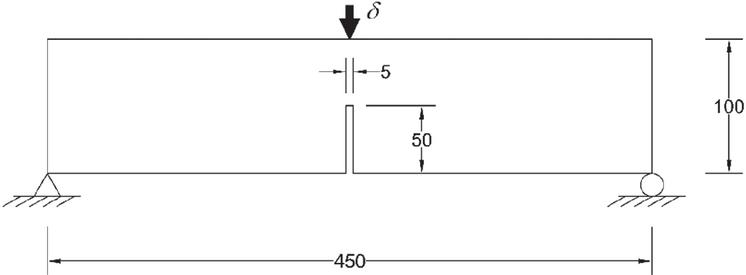
Figure 1 Three-point bending beam used in numerical simulation calculation.

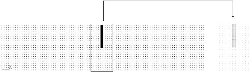
Figure 2 Element-free discretization for a three-point bending beam.

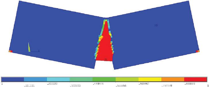
Figure 3 Distribution of damage variable.

The displacement imposed at the center of the top edge of the beam is $u_0=1$ mm. The number of load steps used in the calculation is 100. The material properties of the beam are as follows: Young’s modulus $E=2000\mathrm{N}/{\mathrm{mm}}^2$, Poisson’s ratio $v=0.2$, tension strength ${\sigma }_f=2.4\mathrm{N}/{\mathrm{mm}}^2$ and mode I fracture energy $G_c=0.113\mathrm{N}/\mathrm{mm}$. Figure 3 shows the distribution of damage variable within the problem domain.

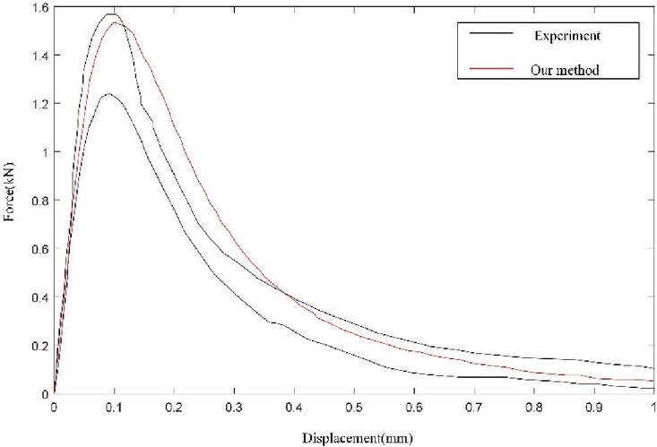
Figure 4 Comparison of load-displacement curves for the three-point bending beam: experiment [35] and numerical simulation.

As can be seen in Figure 4, the calculated results are in good agreement with the experimental results and only show slight differences in maximum load values. The relative error in maximum load values is about 3.2%. Figures 4 and 10 show the results of numerical simulations for the case of the influence domain 2.5 times the nodal spacing and the polynomial degree of the basis function 6. Influence analysis on the size of the influence domain and the discussion of the polynomial order of the basis function are described in detail in [39].

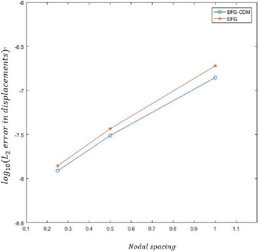
Figure 5 Error estimate in displacements.

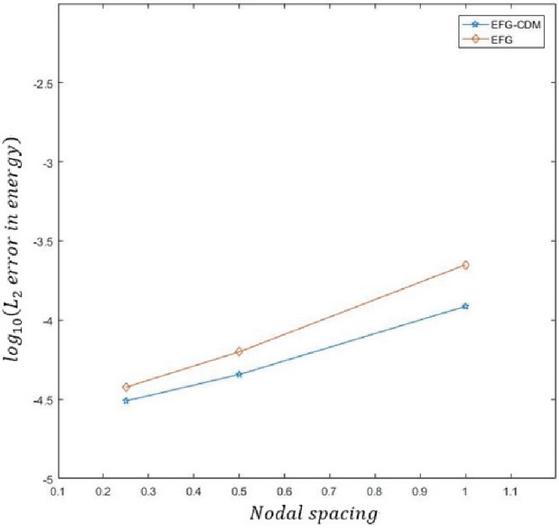
Figure 6 Error estimate in energy.

Figures 5 and 6 show the results of the estimation of the error in displacement and energy using the $L_2$ norm.

4.2 Numerical Simulation of Mixed Mode Failure in a Three-point Bending Beam

To perform simulation calculations for the curved crack growth process, the model is set up as shown in Figure 7. Geometry and boundary conditions of the model are shown in Figure 7. The unit used in Figure 7 is mm. The material properties of the model are: $E=38\mathrm{kN}/{\mathrm{mm}}^2$, $v=0.2,{\sigma }_f=3\mathrm{N}/{\mathrm{mm}}^2$, $G_c=0.069\mathrm{N}/\mathrm{mm}$. The maximum displacement imposed on the top center of the beam is 0.3 mm. Calculation results are compared with experimental results of [36]. Figure 8 shows distribution of the nodes used in numerical calculations. The number of nodes used in this example is 15797. In this simulation, the displacement increment of $\mathrm{\Delta }u=0.001\mathrm{mm}$ is used.

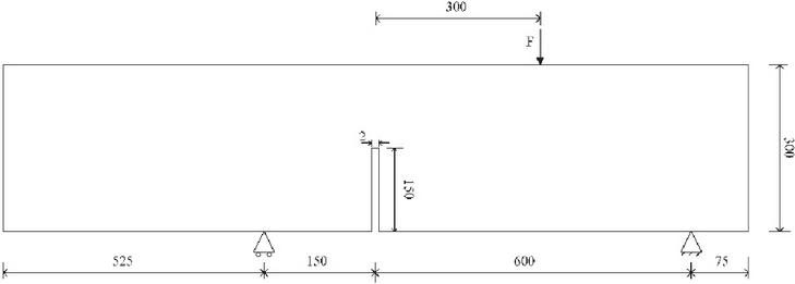
Figure 7 Mixed bending test model.

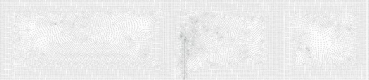
Figure 8 Meshfree nodal discretization for three-point bending beam.

Figure 9 shows the propagation direction and deformed shape of the crack obtained by numerical calculation. As shown in Figure 9, the crack propagation direction agrees with the predicted direction.

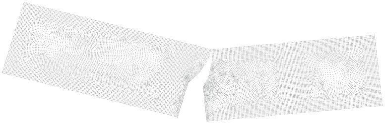
Figure 9 Result of the simulation.

Figure 10 shows a comparison between the experimental results and the numerical simulation results. Figure 10 shows the relationship between load and crack opening displacement, and the experimental and calculated results show good agreement. The relative error in maximum load value is 2.38%.

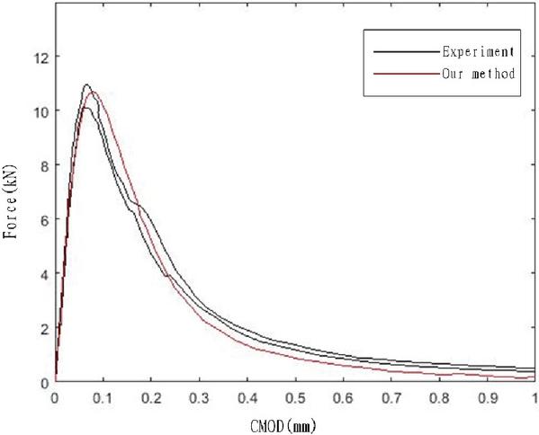
Figure 10 Comparison of results: experiment [36] and proposed method.

Figures 11–13 show the results of the analysis using the $L_2$ norm and $H_1$ norm for error estimation for the mixed crack problem.

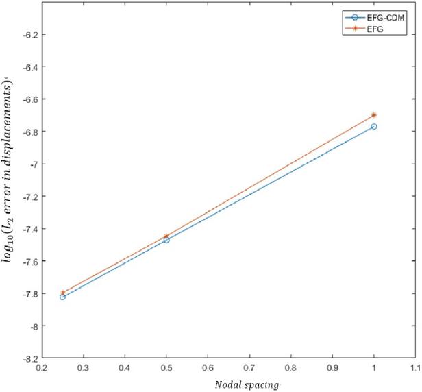
Figure 11 $L_2$ error in displacements with nodal spacing.

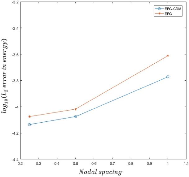
Figure 12 $L_2$ error in energy with nodal spacing.

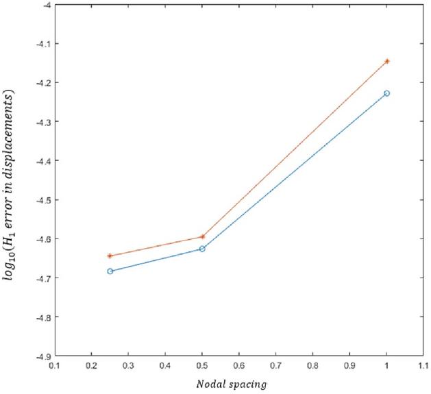
Figure 13 $H_1$ error in displacements with nodal spacing.

5 Conclusions

In this paper, a crack analysis method based on a combination of the EFG method and the CDM method is presented. This method can successfully describe crack initiation and propagation without using specific criteria with smaller nodal distribution. In addition, this method can predict the crack path accurately without using any crack tracking algorithm. It can reduce the number of iterations of some criteria used for evaluation of the influence domain of each node, such as diffraction or visibility criterion used for discontinuities implementation in the meshfree methods. This model is only applied to 2D problems for isotropic materials, but the extension to 3D and anisotropic is theoretically possible.

References

[1] N. Moës and T. Belytschko, Extended finite element method for cohesive crack growth. Engineering Fracture Mechanics 2002, 69(7): 813–833.

[2] T. Belytschko and T. Black, Elastic crack growth in finite elements with minimal remeshing. Int J Numer Methods Engng 1999, 45(5): 601–620.

[3] N. Moës, J. Dolbow and T. Belytschko, A finite element method for crack growth without remeshing. Int J Numer Methods Engng 1999, 46(1): 131–150.

[4] Li X, Chen J. The implementation of the extended cohesive damage model for multicrack evolution in laminated composites. Compos Struct 2016, 139: 68–76.

[5] Simó J C, Oliver J, Armero F. An analysis of strong discontinuities induced by strain-softening in rate-independent inelastic solids. Comput Mech 1993, 12: 49–61.

[6] Oliver J. Continuum modeling of strong discontinuities in solid mechanics using damage models. Comput Mech 1995, 17: 277–296.

[7] Oliver J, Cervera M, Manzoli O. Strong discontinuities and continuum plasticity models: the strong discontinuity approach. Int J Plast 1999, 15: 319–351.

[8] Oliver J, Huespe AE, Samaniego E, Chaves WV. Continuum approach to the numerical simulation of material failure in concrete. Int J Numer Anal Methods Geomech 2004, 28: 609–632.

[9] Oliver J, Huespe AE. Continuum approach to material failure in strong discontinuity settings. Comput Methods Appl Mech Engng 2004, 193: 3195–3220.

[10] Oliver J, Dias IF, Huespe AE. Crack-path field and strain-injection techniques in computational modeling of propagating material failure. Comput Methods Appl Mech Eng 2014, 274(6): 289–348.

[11] Oliver J, Huespe AE, Samaniego E. On strategies for tracking strong discontinuities in computational failure mechanics. Fifth World Congress on Computational Mechanics, 2002, 7–12.

[12] Oliver J, Huespe AE, Samaniego E, et al. Continuum approach to the numerical simulation of material failure in concrete. Int J Numer Anal Meth Geomech 2004, 28(7–8): 609–632.

[13] Areias PMA, Belytschko T. Analysis of three-dimensional crack initiation and propagation using the extended finite element method. Int J Numer Meth Eng 2005, 63(5): 760–788.

[14] Sethian JA. Level set methods and fast marching methods. Cambridge: Cambridge University Press, 1999.

[15] Rabczuk T, Belytschko T, Xiao SP. Stable particle methods based on Lagrangian kernels. Comput Methods Appl Mech Eng 2004, 193(12–14): 1035–1063.

[16] Schweitzer MA. Stable enrichment and local preconditioning in the particle-partition of unity method. Numer Math 2011, 118(1): 137–170.

[17] Rabczuk T, Belytschko T. Adaptivity for structured meshfree particle methods in 2D and 3D. Int J Numer Meth Eng 2005, 63(11): 1559–1582.

[18] Muthu N, Maiti SK, Yan W, et al. Modelling interacting cracks through a level set using the element-free Galerkin method. Int J Mech Sci 2017, 134: 203–215.

[19] Zhuang X, Augarde CE, Mathisen KM. Fracture modeling using meshless methods and level sets in 3D: Framework and modeling. Int J Numer Meth Eng 2012, 92(11): 969–998.

[20] Oliver J, Huespe AE, Samaniego E, et al. Continuum approach to the numerical simulation of material failure in concrete. Int J Numer Anal Meth Geomech 2004, 28(7–8): 609–632.

[21] Belytschko T, Lu YY, Gu L. Element-free Galerkin methods. Int. J. Numerical Methods Eng 1994a, 37: 229–256.

[22] Belytschko T, Gu L, Lu YY. Fracture and crack growth by element-free Galerkin methods. Model Simulat Mater Sci Eng 1994b, 2: 519–534.

[23] Atluri SN, Zhu T. A new meshless local Petrov–Galerkin (MLPG) approach in computational mechanics. Comput Mech 1998, 22(2): 117–127.

[24] Jiun-Shyan Chen, et al. Reproducing Kernel Particle Methods for large deformation analysis of non-linear structures. Comput. Methods Appl. Mech. Engrg 1996, 139: 195–227.

[25] Rabczuk T, Belytschko T. Cracking particles: a simplified meshfree method for arbitrary evolving cracks. Int J Numer Methods Eng. 2004, 61(13): 2316–2343.

[26] Vinh Phu Nguyen, et al. Meshless methods: A review and computer implementation aspects. Mathematics and Computers in Simulation 2008, 79: 763–813.

[27] Liu GR, Gu YT. A point interpolation method for two-dimensional solid. Int J Numer Meth Engng 2001, 50: 937–951.

[28] YT Gu, LC Zhang. Coupling of the meshfree and finite element methods for determination of the crack tip fields. Engineering Fracture Mechanics 2008, 75: 986–1004.

[29] Belytschko T, Organ D. Coupled finite element–element-free Galerkin method. Comput Mech 1995, 17: 186–195.

[30] Hegen D. Element-free Galerkin methods in combination with finite element approaches. Comput Meth Appl Mech Engng 1996, 135: 143–166.

[31] Gu YT, Liu GR. A coupled element free Galerkin/boundary element method for stress analysis of two-dimensional solids. Comput Meth Appl Mech Engng 2001, 190(34): 4405–4419.

[32] Gu YT, Liu GR. Hybrid boundary point interpolation methods and their coupling with the element free Galerkin method. Engng Anal Bound Elem 2003, 27(9): 905–917.

[33] Liu GR, Gu YT. Meshfree local Petrov–Galerkin (MLPG) method in combination with finite element and boundary element approaches. Comput Mech 2000, 26(6): 536–546.

[34] Kumchol Yun et al. An advanced continuum damage mechanics model for predicting the crack progress process based on the consideration of the influence of crack direction under quasi-static load. Int J Mech Sci 2017, 487–496.

[35] Rots JG. Computational modelling of concrete fracture. PhD Thesis. Delft University of Technology, 1988.

[36] Gálvez JC, Elices M, Guinea GV, Planas J. Mixed mode fracture of concrete under proportional and nonproportional loading. Int J Fract 1998, 94(3): 267–284.

[37] Miehe C, Welschinger F, Hofacker F. Thermodynamically consistent phase-field models of fracture: variational principles and multi-field FE implementations. Int J Numer Methods Eng 2010, 83(10): 1273–1311.

[38] Kumchol Yun et al. A modified phase field model for predicting the fracture behavior of quasi-brittle materials. Int J Numer Methods Eng 2021, 1–20.

[39] AR Khoei, M Vahab, H Ehsani and Rafieerad. X-FEM modeling of large plasticity deformation; a convergence study on various blending strategies for weak discontinuities. European Journal of Computational Mechanics, 2015, 24(3): 79–106.

[40] D Colombo and P Massin. Level set propagation for mixed-mode crack advance. European Journal of Computational Mechanics, 2012, 21(3–6): 219–230.

[41] GR Liu, YT Gu. An introduction to meshfree methods and their programming. Springer Dordrecht, Berlin, 2005.

Biographies

Hyo-Song Kim was born in 1992, graduated from Faculty of Mechanics, Kim Il Sung University, DPR Korea, in 2016 and acquired a Ph.D. in Computational Solid Mechanics. Interest fields are structure design, fracture mechanics and computational mechanics.

Jang-Chol Hwang was born in 2002, graduated from Faculty of Mechanics, Kim Il Sung University, DPR Korea, in 2023 and is a graduate student of the faculty of mechanics. Interest fields are computational mechanics and fracture mechanics.

Kumchol Yun was born in 1983, graduated from Faculty of Mechanics, Kim Il Sung University, DPR Korea, in 2004. From 2014 to 2019, Yun researched at Harbin Engineering University. Yun is an expert in the fields of mechanics, obtaining the Ph.D. degree in Damage Mechanics. Interest fields are structure design, fracture mechanics, and computational mechanics.

Jun-Hyok Ri was born in 1986, graduated from University of Sciences in 2006. He obtained the Ph.D. degree from State Academy of Sciences. Interest fields are fracture mechanics, nonlinear optimization and multiscale modeling of composite and damage materials.

Chi-Myong Kim was born in 1984, graduated from Pyongyang University of Transport, DPR Korea, in 2006. Kim has been working as a lecturer at faculty of civil engineering, Pyongyang University of Transport, since 2010. Interest fields are bridge structure design and construction. He obtained the Ph.D. degree from Pyongyang University of Transport.

European Journal of Computational Mechanics, Vol. 34_6, 449–470
doi: 10.13052/ejcm2642-2085.3461
© 2026 River Publishers