Lattice Element Model Elastic Behaviour in Solid Mechanics: Bayesian-Based Calibration and Fine-Tuning
Duje Pavić1,*, Noemi Friedman2, Hermann G Matthies3 and Mijo Nikolić1
1University of Split, Faculty of Civil Engineering, Architecture and Geodesy, Matice hrvatske 15, 21000 Split, Croatia
2HUN-REN Institute for Computer Science and Control (SZTAKI), Kende u.13-17, Budapest, 1111, Hungary
3Institute of Scientific Computing Technical University Braunschweig Brunswick, Germany
E-mail: dpavic@gradst.hr
∗Corresponding Author
Received 23 September 2025; Accepted 13 November 2025
Abstract
This work investigates the elastic behaviour of a mechanical discrete lattice element model based on Timoshenko beam elements. Due to the selected irregular meshes generated with Delaunay triangulation and one-dimensional elements, lattice models struggle to correctly simulate a wide range of elastic material responses, particularly in capturing lateral deformations associated with variations in the material’s Poisson ratio. To address this limitation, we introduce correction coefficients that modify the stiffness properties of the lattice beam elements, influencing the global mechanical behaviour of the lattice. A Bayesian stochastic identification framework is chosen to calibrate these coefficients using a set of standard mechanical tests, ensuring consistency with the proper continuum elastic response. The applicability of the identified lattice element stiffnesses is evaluated across different loading conditions and material properties. The methodology ensures a fine tuning of the model, accuracy in simulating mechanical deformations, and the basis for non-linear phenomena, crack initiation and its propagation across the lattice.
Keywords: Lattice element model, Bayesian inference, elastic response, parameter identification, polynomial chaos method.
1 Introduction
Lattice element models, as a class of discrete element models [7, 2, 9, 12, 33, 34, 35], have become a robust tool for simulating the behaviour of quasi-brittle heterogeneous materials, such as rocks, concrete, and ceramics, particularly in capturing the complex internal processes associated with fracture propagation. Alongside advanced approaches such as Extended Finite Element Models (X-FEM) and Embedded Discontinuity Finite Element Models (ED-FEM) [1, 4, 5], lattice models offer distinct advantages, including the natural incorporation of material heterogeneity, fracture representation and crack development across multiple scales, from macroscopic to mesoscopic and microscopic phenomena [6]. However, their use of one-dimensional elements limits the ability to fully capture elastic behaviour, particularly for materials with a wide range of Poisson’s ratios. The input (lattice element) elastic parameters often fail to reproduce the material’s overall elastic response [16], while mesh irregularity and random particle positioning introduce oscillatory deformation patterns compromising elastic uniformity of mesh deformations. Although such non-uniform fields may beneficially reflect material heterogeneity and micro-defects, voids or initial cracks, they introduce local weaknesses that cause stress concentrations and variability in stress-strain fields [14, 17, 13, 3, 38]. Micro-defects pose a challenge in achieving continuum equivalence in the linear elastic phase under homogeneous loading, as the lattice inherently captures these local non-uniformities while the continuum model assumes a uniform response without such variability.
As shown in [8], lattice models are capable of reproducing continuum elastic responses when properly configured, or calibrated, by using the concept of continuum equivalence, where the discrete lattice network replicates the stress-strain behaviour of a homogeneous elastic medium. For regular lattice configurations, continuum equivalence can be achieved through analytical calibration of lattice element stiffnesses providing elastic uniformity. This results in a global and local match in deformation and stress fields. However, regular meshes introduce geometric bias, which can significantly affect fracture simulations by constraining crack paths along predefined directions. On the contrary, irregular and random lattices are commonly used in fracture modelling, as they reduce mesh-induced crack paths. However, these irregular mesh configurations complicate the accurate reproduction of elastic behaviour. For example, Rigid Body Spring Models (RBSMs), using translational and rotational degrees of freedom to rigid bodies and multiple interface springs can reproduce elastic uniformity even on irregular meshes [12, 14]. However, simulating lateral deformations for a wide range of Poisson’s ratio requires corrections in RBSM models, such as the fictitious force approach [16], which iteratively adjust the nodal forces to recover the desired elastic response without modifying the lattice stiffness matrix. Alternatively, beam lattice models [10, 9] and the Lattice Discrete Particle Model (LDPM) [11] require calibration of stiffnesses to represent accurate elastic behaviour. In the beam-type lattice models, the axial and bending stiffnesses of the beam elements need to be calibrated to match the required Young’s modulus and Poisson’s ratio, with elastic uniformity even in random lattice geometries. Similarly, in LDPM, the normal and shear stiffnesses of the facet connections are analytically related to the macroscopic elastic properties, and calibrated accordingly to achieve continuum equivalence despite the irregular mesh. Generally, a proper stiffness calibration is essential for reproducing realistic material behaviour in lattice based models prior to fracture.
This paper focuses on refining the Timoshenko beam discrete lattice element model [15] to enhance the accuracy of fracture process simulations by improving their elastic response. In the proposed approach, we introduce the correction coefficients, , , and , into the beam kinematics, which modify the beam element stiffnesses in axial, transversal, and rotational direction. The proper choice of correction coefficients enhances the elastic fidelity of the model. This work proposes a Bayesian stochastic identification of correction coefficients that serve for the calibration of beam element stiffnesses and fine-tuning of the lattice element model. The correction coefficients are treated as uncertain parameters with random variables [19, 20, 21], initially characterized by prior distributions which reflect existing knowledge and assumptions. The Bayesian approach provides a posterior distribution by integrating the prior distribution with observational data to enhance parameter understanding. Unlike deterministic methods, which produce a single solution, this probabilistic framework provides a comprehensive distribution of possible outcomes, improving the reliability and accuracy of the calibration process [22, 26]. To compute the posterior distribution, sampling techniques such as the Markov Chain Monte Carlo (MCMC) method, are often used [28], or some alternative approaches such as Kalman filter methods or Minimum Mean Square Estimators. However, for complex problems like fracture mechanics, the computational demands of Bayesian calibration can be significant. To improve efficiency, complex deterministic models are often replaced with surrogate models, such as the generalized Polynomial Chaos Expansion (gPCE) [23, 24, 25]. gPCE models have proven to be an optimal choice in modelling the parametric dependence of structural responses. The gPCE surrogate was selected for its efficiency in the linear elastic regime, where polynomial expansions and Quasi-Monte Carlo (QMC) sampling enable accurate training and Sobol sensitivity analysis. In cases where gPCE approximations are insufficient, machine learning models, such as neural networks or Gaussian Process Regression (GPR) provide superior performance, particularly for non-linear extensions [27, 36, 37]. Sobol sensitivity analysis is employed to assess the influence of each parameter on the model output, aiding in the optimization of experimental design by quantifying the parameter sensitivity to specific measurements[29, 30].
Furthermore, we investigate homogeneity and isotropy indices of the resulting elastic fields, as shown in [18]. To support fracture simulations, we generate optimal random lattice networks based on Voronoi tessellations, selected to achieve an optimal fit between homogeneity and isotropy. Within these networks, deformation oscillations are constrained to remain within acceptable bounds, ensuring a mesh structure that is both elastically robust and geometrically unbiased for simulating crack propagation.
This work proposes a lattice model calibration on a few numerical experiments based on standard mechanical tests, including a uniaxial tension and a shear test, as well as a beam bending test. It investigates how local stiffnesses of the beam elements change in order to represent various lateral deformations of the lattice model related to material Poisson’s ratio. It further considers the consistency of calibrated coefficients for different tests and load cases.
In these tests, virtual or, so-called synthetic, measurements from a solid Finite Element Method (FEM) model are employed to identify correction coefficients. The stochastic approach with a large number of simulations, as well as Sobol sensitivity analysis, provides in-depth knowledge on the behaviour of lattice model across a range of selected parameter space.
Section 2 details the limitations and introduces the correction coefficients in formulation of the Timoshenko beam lattice model. Section 3 provides an in-depth explanation of Bayesian parameter identification for the Timoshenko beam lattice model. Section 4 discusses numerical examples, offering a direct comparison of the differences between lattice and solid FEM models for each case. Section 5 summarizes the conclusions of the study.
2 Discrete Timoshenko Beam Lattice Element Model
The proposed discrete lattice model is based on Voronoi tessellation, with Timoshenko beam elements placed along the edges of the corresponding Delaunay triangulation (Figure 1(a)). These elements represent cohesive links between neighbouring Voronoi cells, while beam stiffnesses are determined by the geometry, specifically the common edge lengths of adjacent cells (Figure 1(b)) [39, 15]. The disordered mesh structure is appropriate for capturing material heterogeneity and multiphase material, and is well suited for fracture simulation. As shown by Vaiani et al. [18], Delaunay-based lattices offer an optimal balance of homogeneity and isotropy, essential for realistic crack propagation modelling.
While regular lattices offer high homogeneity and elastic uniformity due to symmetry and equal beam lengths, their low isotropy can bias fracture paths [8]. On the contrary, irregular and disordered meshes, with randomly positioned nodes and varying beam orientations, better capture isotropic behaviour and reduce mesh-dependent cracking, but exhibit non-uniform deformation under uniform loading [12, 10].
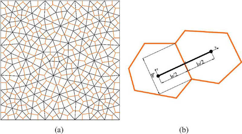
Figure 1 (a) Irregular lattice domain with Voronoi tessellation and dual Delaunay triangulation (b) Two neighbouring Voronoi cells.
Additionally, the one-dimensional structure of the lattice element model and its corresponding lattice element stiffnesses can represent only limited range of elastic responses and lateral deformations associated with Poisson ratio. To improve the lattice model and ensure the lattice reproduces correct global elastic behaviour (e.g., Young’s modulus and Poisson’s ratio), we introduce correction coefficients, , , and adjusting axial, shear, and bending stiffnesses of beam elements, respectively [32]. These corrections allow the model to replicate correctly the deformation fields and wide range of Poisson ratio, even in irregular lattices, while local input elastic parameters such as the element-level Young’s modulus ( ) and Poisson’s ratio ( ) match the global response of the material, defined by the Young’s modulus () and Poisson’s ratio () (Figure 2) [16, 14].
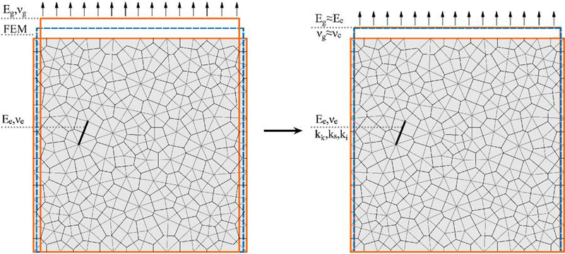
Figure 2 Comparison of lattice model behaviour before and after correction coefficient calibration against solid FEM model. and denote the target global (macroscopic) Young’s modulus and Poisson’s ratio of the material, respectively, while and represent the local (element-level) Young’s modulus and Poisson’s ratio assigned to the Timoshenko beam elements.
2.1 Lattice Index
The Lattice Index combines homogeneity and isotropy, evaluating the overall quality of the lattice mesh [18]. The Lattice Index () is defined as the product of the Homogeneity Index () and the Isotropy Index ():
| (1) |
Homogeneity is calculated by measuring the deviation of the beam lengths from their mean value, identifying a uniform length distribution. The Homogeneity Index () quantifies the uniformity of beam lengths in the network, if it is close to 1 indicating a highly uniform length distribution. It is defined as:
| (2) |
where:
• is the mean absolute deviation of the lengths of the beams, with being the length of the th beam and represents the average length of all non-boundary beams .
• is the average beam length.
Isotropy is calculated by measuring the deviation of the angular distribution from the uniform expectation and assessing orientation uniformity. The Isotropy Index () measures the uniformity of beam orientations across angular sectors (domain is subdivided in equally distributed angular sectors), when a value close 1 indicates a highly isotropic orientation distribution. It is defined as:
| (3) |
where:
• is the mean absolute deviation of the percentage of beams in each sector, with being the percentage of beams in the -th sector and the uniform percentage for sectors.
• is the minimum possible mean absolute deviation for sectors.
2.2 Kinematics of Timoshenko Beam Element
In this paper a Timoshenko beam as lattice element is considered as a basis for the lattice model [15, 31].
The generalized displacement vector for a Timoshenko beam finite element of length and cross-section is defined as:
| (4) |
where: is the longitudinal (axial) displacement along the beam’s length, is the transversal displacement perpendicular to the beam axis, andis the rotation.
For a two-node element, as shown in Figure 3, the nodal displacement vectors are , , and , forming the total nodal displacement vector:
| (5) |
These displacements are interpolated using linear shape functions:
| (6) |
where ranges from 0 to . The displacement fields are expressed as:
| (7) |
with , , and being the respective shape function matrices based on and .
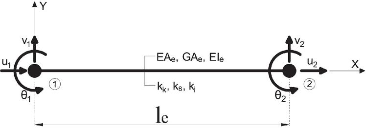
Figure 3 Timoshenko beam with standard degrees of freedom and implemented correction coefficients.
The strain measures for the Timoshenko beam are:
| (8) |
Where is the normal (axial) strain, the shear strain, and the curvature. These strains relate to nodal displacements via the strain-displacement matrix :
| (9) |
Using linear shape functions, the derivatives are:
| (10) |
The strain-displacement matrix is:
| (11) |
This matrix connects strains to displacements. The generalized element stress vector follows the standard formulation of Timoshenko beam models, with the stress resultant vector encapsulating internal forces and moments as:
| (12) |
where is the axial force, the shear force, and the moment. The constitutive relationship is:
| (13) |
where is the diagonal stiffness matrix:
| (14) |
where is the axial stiffness, the shear stiffness (with , where is Poisson’s ratio), and the bending stiffness (with for a rectangular section of height and width 1). In Timoshenko beam theory, the shear correction factor of 0.85 for rectangular cross-sections accounts for the non-uniform distribution of shear stress across the section [40]. The shear correction factor adjusts the average shear stress to better represent the effective shear stiffness of the section.
Introduced correction coefficients , , and modify the stiffness matrix, enabling the lattice model to exhibit global elastic behaviour that closely aligns with plane stress solid models.
| (15) |
The external nodal forces are related to the nodal displacements through the element stiffness matrix as:
| (16) |
where represents the external nodal forces and moments, and is the nodal displacement vector. The stiffness matrix is computed as:
| (17) |
with as the strain-displacement matrix, the diagonal stiffness matrix (incorporating correction coefficients , , ), and the element length.
3 Bayesian Parameter Identification for Timoshenko Beam Lattice Model
3.1 Stochastic Model Formulation
To overcome the limitations noted in Section 2, we use a stochastic approach to identify correction coefficients that are ensuring that lattice models accurately reflect observed structural responses, accounting for uncertainties such as material imperfections, geometric variations, and load inconsistencies. These correction coefficients are treated as random variables to capture this uncertainty, forming a random vector , where is the sample space of all possible outcomes, and corresponds to the three coefficients. This is mathematically expressed as:
| (18) |
where represents a specific realization. The randomness in reflects our incomplete knowledge about the true values. We assign a joint prior distribution to quantify this initial uncertainty, based on engineering judgment or preliminary data [19, 26]. Assuming independence among , , and , joint probability function can be expressed as:
| (19) |
where each is the marginal prior, often chosen as a uniform distribution over a plausible range or a Gaussian distribution, reflecting our prior knowledge [19]. This stochastic approach transforms the deterministic Timoshenko beam equations into a probabilistic model. The governing equations, which relate displacements to external forces , now become random variables:
| (20) |
where is a stochastic operator incorporating the random vector . For each , the displacement depends on the specific values of , , and , as well as . To integrate this stochastic framework with the equilibrium Equation (16), we reformulate the nodal equilibrium condition stochastically as:
| (21) |
where is the random stiffness matrix, with incorporating the random correction coefficients , , and .
3.2 Surrogate Modelling with gPCE
Simulating fracture and failure in materials even when using lattice models can be computationally intensive, particularly for large lattices, leading to significant time demands. Consequently, solving the Bayesian inverse [21] problem using the MCMC method [28] (Section 3.4) can become prohibitively slow due to these computational challenges. To overcome this, we use a surrogate model based on the gPCE [23, 24], which approximates the complex relationship between the input parameters and the output displacement field . The gPCE model approximates , the parametric description of the displacement filed, the so called forward model , as a series:
| (22) |
where are orthogonal polynomial basis functions selected based on the distribution of and are coefficients to be determined. The vector contains all polynomial coefficients. As we don’t have any prior knowledge or engineering judgment of parameters we assumed a uniform distribution for all correction coefficients in physically reasonable ranges. The polynomial degree determines the number of terms , balancing accuracy and computational cost. To compute the coefficients , we employ QMC sampling technique, generating . Then samples are split into fitting points for constructing the model and validation points for assessing the model’s performance. The coefficients are obtained through a least-squares regression by solving:
| (23) |
where is a matrix of polynomial evaluations at the fitting points, with columns corresponding to the basis functions and rows to the sample points, while is the displacement data used for fitting [27]. This regression minimizes the error between the true displacements and the gPCE approximation, the true displacements being from the lattice model. The fit quality is assessed by minimizing the mean squared error:
| (24) |
which measures the average squared difference between the true and approximated displacements.
3.3 Sobol Sensitivity Analysis
Sensitivity analysis is key to understanding how variations in , , and affect the displacement field . Sobol analysis aids in experiment design, sensor placement, and identifying influential parameters by computing Sobol indices, which quantify the contribution of individual or combined input parameter variations to the total variance of [30]. The total variance of is estimated from the gPCE coefficients, and partial variances and are calculated for individual parameters and pairs . The first-order Sobol index captures the sensitivity to a single parameter, while the second-order index reflects interactions between two parameters. These are defined as:
| (25) |
where denotes all parameters except , is the total variance, and , are partial variances. The gPCE’s orthogonality allows direct computation of these variances from the coefficients :
| (26) |
where is the set of multi-indices corresponding to polynomials depending only on , and is the norm of the polynomial basis . This approach speeds up analysis by using a surrogate model to replace costly deterministic model sampling, enabling efficient sensitivity assessment across the parameter space [30, 29].
3.4 Bayesian Parameter Identification
The Bayesian approach updates [22, 25] our knowledge of , , and using observed displacement data . Starting with the prior , which contains our initial assumptions of the parameters, we refine it to a posterior using Bayes’ theorem:
| (27) |
where is the likelihood, expressing how likely it is to observe the measured value given a certain value of the parameters , is the prior distribution function of the parameters representing our initial knowledge, is the posterior distribution, representing our change knowledge about the correction coefficients after assimilating the measurement , and is the evidence, the normalization constant. Since measurements include noise, we model as:
| (28) |
where and is Gaussian noise with covariance . Assuming a perfect forward model, the likelihood for a given value of the parameter is obtained by evaluating the probability density of the Gaussian noise at the discrepancy between the measured and the computed displacements.
| (29) |
In most cases, the posterior distribution cannot be expressed analytically, prompting the development of various mathematical techniques, such as sampling methods, to approximate its shape. These sampling techniques generate samples that converge to a stationary distribution aligned with the target posterior distribution. In this paper, MCMC method, specifically employing the Metropolis-Hastings algorithm [28], is selected for its robustness and simplicity nature. This approach leverages a random walk strategy to efficiently collect samples from the desired posterior distribution.
4 Numerical Examples and Results
To identify correction coefficients for enhancing the Discrete Lattice Element model, three standard mechanical tests were selected: tensile test, shear test, and three-point bending test. These tests were chosen due to their widespread use in determining the mechanical properties of materials. The Timoshenko beam lattice model enriched with correction coefficients, was implemented in the Finite Element Analysis Program (FEAP) to generate the results [41]. For this study, synthetic measurements derived from a solid FEM model were employed, providing a known “true” value to calibrate the lattice model with correction coefficients. The solid reference model is a plane stress FEM model using 3-node linear triangular elements with an unstructured, fine mesh for simulating the continuum elastic response under the prescribed loading. The material is assumed isotropic linear elastic with Young’s modulus kN/cm2 and Poisson’s ratio varying from 0 to 0.4 across tests. This model was selected as the “true” reference because it provides a homogeneous, isotropic stress-strain field approximating the analytical continuum solution, free from the discretization artifacts and irregularities of lattice models, thus enabling accurate synthetic displacement measurements for Bayesian calibration [41]. The construction of gPCE models and MCMC analysis was performed using the open-source stochastic library SGLIB [42]. This study focuses on the linear elastic behaviour of the samples, which requires only a single calculation step, ensuring minimal computational time. In the following sections, we detail the specifications of each test sample, the selected measurements, and the behaviour of the correction coefficients across each test. Two mesh densities (coarse with 1898 elements and fine with 5755 elements) were evaluated for mesh sensitivity specifically in the tension test, while the shear and bending tests used a single mesh density (1898 elements for shear, 4055 elements for bending).
4.1 Tension Test
Tensile tests were performed on two square samples, each with a 15 cm side length, identical geometries, boundary conditions, and mechanical properties, but differing in mesh configurations, as shown in Figure 4. A uniform tensile load was applied to both samples. The irregular structure of the lattice model is expected to exhibit heterogeneous behaviour, resulting in non-uniform displacements under uniform loading, as discussed in Section 2. The tests employed two distinct mesh densities to evaluate their influence on the correction coefficients. The Timoshenko beams in the lattice model were defined with elastic properties kN/cm2 and .
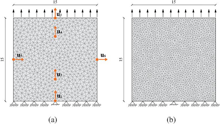
Figure 4 Uniaxial tension test meshes with measurements , and : (a) Mesh-1 with 1898 elements (b) Mesh-2 with 5755 elements. , , .
Three measurements (, and ) were used for model evaluation, based on relative differences at positions marked by orange dots in Figure 4. Synthetic reference values, considered as “true” values, were obtained from a solid FEM model with the same domain shape, boundary conditions, and material properties.
4.1.1 Local representation of deformations
Mesh quality is quantified using the index L, the product of homogeneity and isotropy. Mesh-1 has L0.82, while the denser Mesh-2 achieves a higher value of L0.9 due to more uniform beam lengths and orientations (Figure 5). While Mesh Index has limited influence on global elastic behaviour, it affects local stress concentrations and deformation patterns, as well as elastic uniformity. Homogeneity ensures consistent beam lengths, while isotropy promotes direction-independent mechanical responses, especially relevant for unbiased crack propagation. Although complete elastic uniformity is not achieved due to mesh randomness, it remains within acceptable bounds.
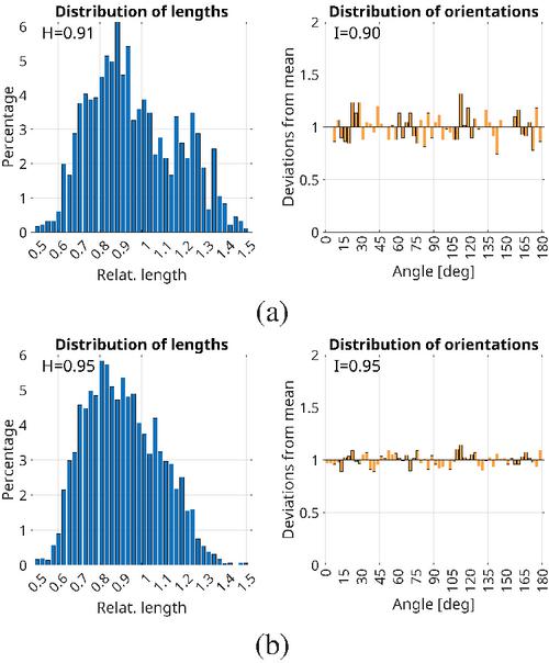
Figure 5 Homogeneity and isotropy indices (a) Mesh-1 with 1898 elements (b) Mesh-2 with 5755 elements.
4.1.2 Surrogate gPCE model training
Given the absence of prior knowledge about the behaviour of the correction coefficients, a uniform distribution (U(0.1, 2.5)) was selected for all three coefficients to reflect equal uncertainty for all coefficient values. QMC sampling was utilized to generate two datasets from this distribution: a training set of 1500 samples for constructing the gPCE model and a test set of 500 samples for validating its accuracy. The lattice model’s response was computed at the designated measurement points for each sample, requiring only a single time step per calculation. Leveraging a cluster computer, all 2000 samples were processed in a few minutes. While 2000 samples were used here for robust training and validation in the linear case, future non-linear applications may benefit from more sample-efficient surrogates like neural networks or GPR, as discussed in Section 1. The best-fitting gPCE model was determined by evaluating and comparing the maximum absolute errors (MAE) between training and test samples for different polynomial degrees. MAE was calculated as the difference between the gPCE model’s predictions and the lattice model’s results at the measurement points.
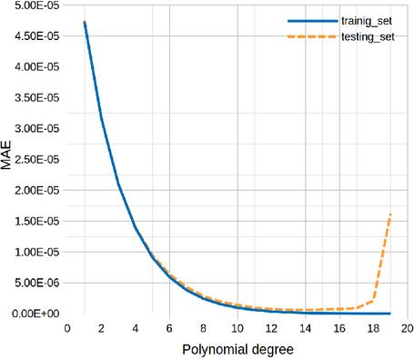
Figure 6 Accuracy assessment of the gPCE surrogate model based on polynomial degree for tension test.
As shown in Figure 6, for linear behaviour, the error of the gPCE model decreases with increasing polynomial degree for the samples on which it was trained (1500 samples). Therefore, a set of testing samples were used to validate the gPCE model (500 samples). As it can be seen, the gPCE model’s performance on the validation samples diverges from the training sample beyond a specific polynomial degree due to the fixed, limited number of training samples. As a result, a 13th-degree polynomial was chosen, resulting in 560 polynomial coefficients.
Table 1 summarizes the Sobol sensitivity indices obtained from the gPCE surrogate model. The analysis reveals that beam longitudinal and shear stiffness have the most significant impact on the measurements, whereas bending stiffness shows no notable influence. In the third measurement, shear stiffness exhibits a markedly greater effect, attributed to its role in capturing the lateral straining of the sample.
Table 1 Linear Sobol sensitivity indices – tension case
| measurement | |||
| 0.9717 | 0.0283 | 0.0000 | |
| 0.9773 | 0.0227 | 0.0000 | |
| 0.7771 | 0.2229 | 0.0000 |
4.1.3 Identification of coefficients and displacements results
The MCMC identification process estimates model parameters by aligning them with synthetic measurements, incorporating a 1% measurement error based on strain gauge precision and literature [20]. Modelling error is derived from differences between proxy models and test data, and both error sources are combined in the total error distribution.
As shown in Figure 7(a), MCMC results confirm the identifiability of the correction coefficients for longitudinal and shear stiffness, with low variability. In contrast, the bending stiffness coefficient shows large uncertainty, indicating it cannot be reliably identified from the experiments used. The analysis was conducted using 10 Markov chains with 4000 steps each.
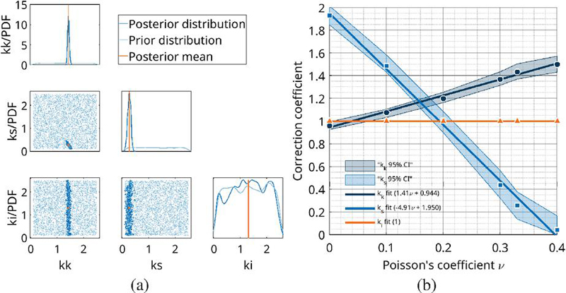
Figure 7 (a) Posterior distributions of the correction coefficients - tension case; kN/cm2 and (b) Mean and confidence intervals (CIs) of updated correction coefficients as a function of the Poisson’s ratio, and the linear mean approximation; marked points are posterior mean.
To better illustrate the relationships among the correction coefficients, a visualization of their posterior distributions was created for a fixed input Poisson’s ratio of 0.33, as shown in Figure 8. This figure overlays the probability density functions (PDFs) for , , and . The plot reveals that has the narrowest distribution, shows moderately broader spread, and exhibits the widest variation with substantial uncertainty [37].
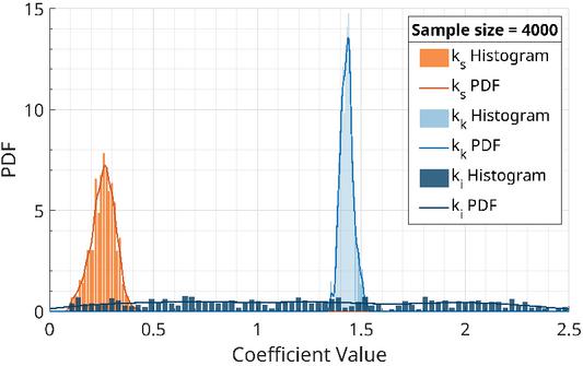
Figure 8 PDFs of correction coefficients for Poisson’s ratio of 0.33.
Table 2 Correction coefficients identification results – tension case
| Posterior mean | 1.4331 | 0.2585 | 1.2634 |
| Posterior st. dev. | 0.0319 | 0.0599 | 0.6492 |
| Posterior mean | 1.4688 | 0.2564 | 1.1828 |
| Posterior st. dev. | 0.0355 | 0.0622 | 0.6913 |
| Note: for kN/cm2, | |||
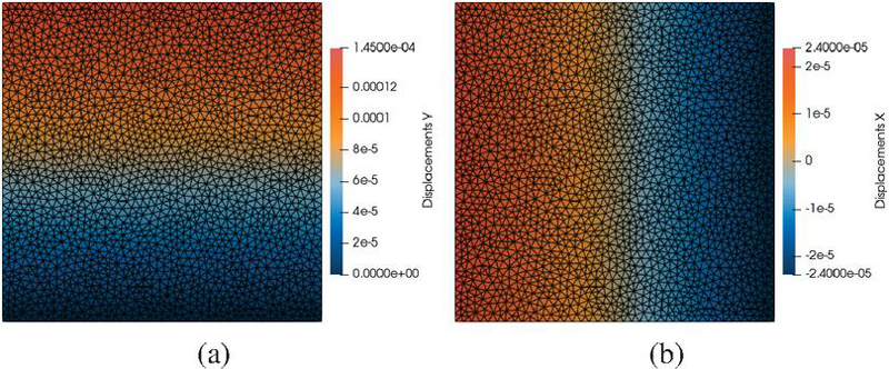
Figure 9 Displacements of solid plane stress FEM model for tension test ( kN/cm2 and ), Mesh-2: (a) Y direction (b) X direction.
The identified correction coefficients are consistent across different mesh densities (Mesh-1 and Mesh-2) (Table 2), indicating that mesh refinement has minimal impact on calibration results. However, the coefficients vary significantly with changes in Poisson’s ratio, meaning a new calibration is required for each desired Poisson ratio. As Poisson’s ratio increases, the longitudinal stiffness correction increases (from 0.96 to 1.52), while the shear stiffness correction decreases (from 1.93 to 0.1) (see Figure 7(b), where the shaded areas represent uncertainty ranges with 95 % confidence intervals). The bending stiffness remains unidentifiable in the current setup. These coefficients enable the lattice model to reproduce the elastic behaviour of solid FEM models, independent of mesh layout but dependent on material properties.
With the identified coefficients implemented, we obtain the calibrated response of the lattice model. Specifically, as shown in Figures 9 and 10, the calibrated model effectively simulates displacements in both Y and X directions under the tension test, when compared to the solid plane stress FEM model. Furthermore, Figure 11 highlights magnitude percentage errors in nodal displacements between the two models for both meshes. While errors are generally low, a closer look at Figures 11(a) and (b) reveals notably higher values particularly near the fixed boundaries. This increase occurs because the lattice model’s irregular beam structure struggles to enforce near-zero displacements in these regions, leading to amplified relative errors and causes some minor local errors in the interior regions across the domain.

Figure 10 Displacements of lattice model with integrated correction coefficients for tension test ( kN/cm2 and ), Mesh-2: (a) Y direction (b) X direction.
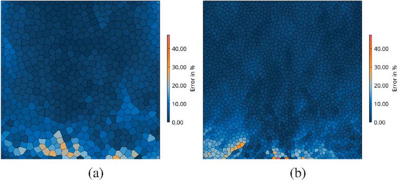
Figure 11 Magnitude percentage error in nodal displacements between the two models for kN/cm2 and , with nodes represented by their Voronoi diagrams: (a) Mesh-1, (b) Mesh-2.
4.2 Shear Test
A shear test was conducted on a square sample with identical dimensions to those used in the tensile test. The sample was fixed at its base and subjected to a uniform horizontal load along the upper edge to simulate shear conditions. Four measurements (, , and ) were used to determine the correction coefficients (Figure 12). As with the tensile test, the measurement values were derived from a solid plane stress FEM model to represent synthetically measured or true values.
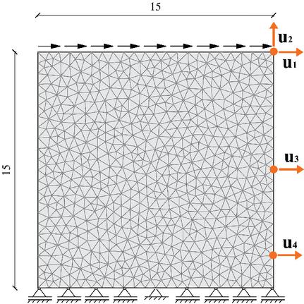
Figure 12 Shear test mesh (Mesh-1 with 1898 elements) with measurements , , and .
For the shear test, correction coefficients were determined in the same process as in the tension test: a uniform distribution U(0.1, 2.5) for all three coefficients uncertainty, 2000 QMC samples (1500 for training, 500 for validation) for the gPCE model. As with the tension test, a 13th-degree polynomial with 560 coefficients was used.
Table 3 displays the sensitivity indices for each parameter across specific measurements. Longitudinal stiffness dominates in the first and second measurements, while shear stiffness has minimal impact. In the third and fourth measurements, shear stiffness shows much greater influence. Bending stiffness consistently exhibits negligible influence across all measurements.
Table 3 Linear Sobol sensitivity indices – shear case
| measurement | |||
| 0.9408 | 0.0592 | 0.0000 | |
| 0.9752 | 0.0247 | 0.0000 | |
| 0.8861 | 0.1139 | 0.0000 | |
| 0.5769 | 0.4231 | 0.0000 |
Similar to tension test, Figure 13(a) illustrates that the MCMC approach produced a narrow posterior distribution for longitudinal and shear stiffness, effectively identifying their correction coefficients. In contrast, the bending stiffness exhibited a broad posterior distribution, indicating that it could not be accurately determined. Results from MCMC identification are: , shear stiffness .
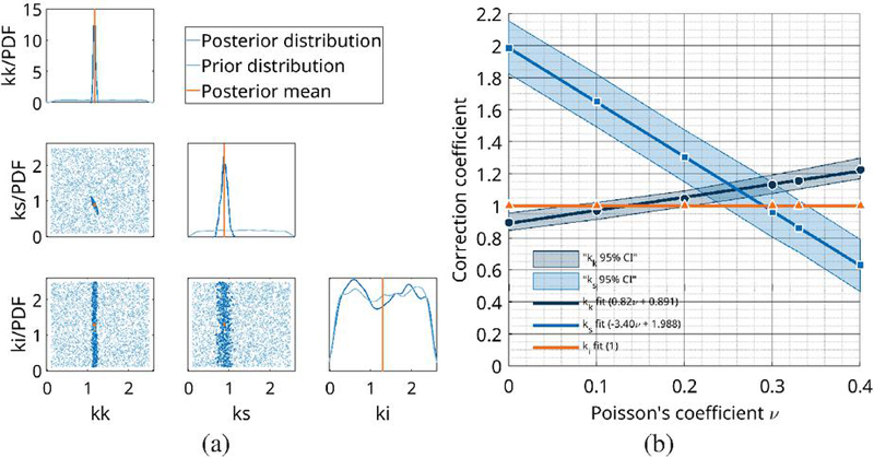
Figure 13 (a) Posterior distributions of the correction coefficients - shear case; kN/cm2 and (b) Mean and confidence intervals (CIs) of updated correction coefficients as a function of the Poisson’s ratio, and the linear mean approximation; marked points are posterior mean.
As in the tension test, the correction coefficients for longitudinal stiffness increase (from 0.89 to 1.22), while those for shear stiffness decrease (from 1.98 to 0.63) as Poisson’s ratio increases from 0 to 0.4 (see Figure 13(b)). However, the correction coefficients values obtained from the shear test differ from those derived from the tensile test. Thus, for identical geometry and mesh, the correction coefficients are influenced by the type of test (boundary conditions), which affects the sample’s behaviour and, consequently, the correction coefficients.
4.3 Three-Point Bending Test
A three-point bending test was conducted on a beam measuring 100 cm in length and 10 cm in height. The beam was supported by a hinge bearing on the left side and a sliding bearing on the right side, with a concentrated vertical force applied at the midpoint of the span. For this test, the lattice mesh with 4055 elements achieved a Mesh Index of , indicating that Delaunay triangulation produced a well-balanced network with high levels of homogeneity and isotropy . Three measurements (, and) were used to determine the correction coefficients (Figure 14). These measurement types and locations were chosen to optimize sensitivity of correction coefficients, as measurements selection has great impact on identification accuracy of coefficients. As in previous tests, measurement values from the solid plane stress FEM model were taken as the reference true values.
Figure 14 Three point bending test mesh with 4055 elements and with measurements , and .
For the three-point bending test, same process (see Section 4.1.2) is used in determining correction coefficients: a uniform distribution U(0.1, 2.5) for longitudinal stiffness and shear stiffness , and U(0.1, 5.0) for bending stiffness . The gPCE model used 5000 QMC samples (4000 for training, 1000 for testing). Minimum error was achieved with an 18th-degree polynomial (1330 coefficients).
Sobol sensitivity indices obtained from the gPCE model are shown in Table 4. Longitudinal stiffness has the greatest influence across all three measurements, while shear stiffness shows negligible impact. The third measurement exhibits significant sensitivity to bending stiffness, reflecting its role in the rotation of the sample’s edge faces.
Table 4 Linear Sobol sensitivity indices – bending case
| measurement | |||
| 0.9806 | 0.0192 | 0.0002 | |
| 0.9218 | 0.0765 | 0.0017 | |
| 0.6559 | 0.0870 | 0.2571 |
For this test, MCMC results confirm the successful identification of all three correction coefficients, with low variability for longitudinal and bending stiffness, and moderately higher variability for shear stiffness, shown Figure 15(a). Consistent with the previous tests, correction coefficients exhibit similar behaviour with changes in Poisson’s ratio, as shown in Figure 15(b). As Poisson’s ratio increases from 0 to 0.4, longitudinal stiffness correction coefficients slightly increase (from 1.02 to 1.10), while shear stiffness coefficients decrease (from 1.18 to 0.77) and bending stiffness coefficients decrease (from 1.56 to 0.32).
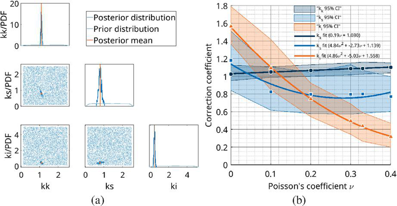
Figure 15 (a) Posterior distributions of the correction coefficients - bending case; kN/cm2 and (b) Mean and confidence intervals (CIs) of updated correction coefficients as a function of the Poisson’s ratio, and the linear mean approximation for and non-linear for and ; marked points are posterior mean.
Results in terms of posterior mean values from MCMC identification are: , shear stiffness , and (Figure 15(a)). Compared to the tensile and shear tests, these coefficients exhibit different values, indicating that correction coefficients are specific to the sample’s geometry and the type of mechanical test that is conducted.
Figure 16 shows direct comparison of the displacement fields of the solid model and the calibrated lattice model. The model calibrated with selected measurements correctly simulated deflections and deformations of the beam, except for the left and right boundary surfaces and their corresponding inclinations (Figure 16(c)), where errors are present. This is due to the lattice model limitations and inability to capture both, deflections and side rotations in beam bending example.
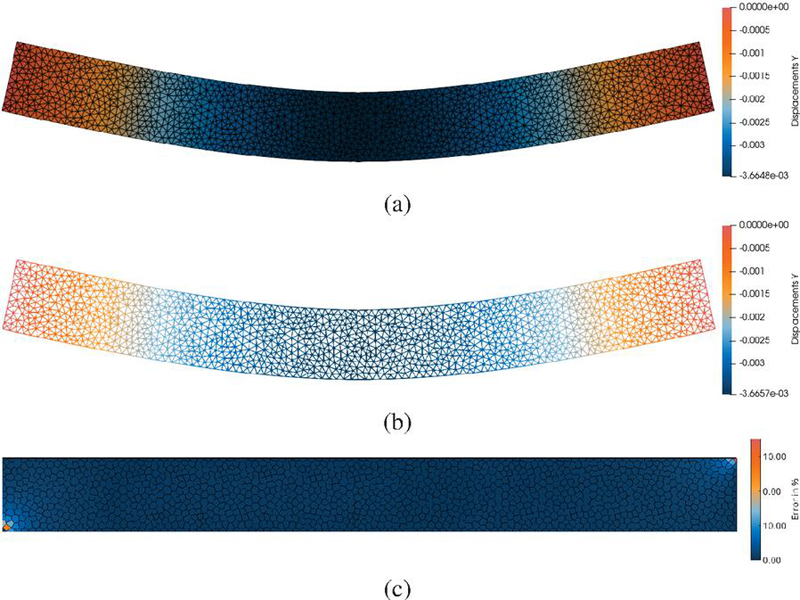
Figure 16 Displacements and errors in the Y direction for a three-point bending test: (a) Solid plane stress FEM model (deformed configuration), (b) Calibrated Timoshenko beam lattice model (deformed configuration), (c) Magnitude percentage error in nodal displacements between the two models, with nodes represented by their Voronoi diagrams.
4.4 Joint MCMC Test
The integrated multi-test calibration aims to combine data from tension, shear, and bending tests to create a single set of correction coefficients (, ,) that can be applied across different conditions, exploring whether this set of coefficients can be universal despite the evident differences in correction coefficients between these three tests. This approach utilizes pre-existing gPCE surrogate models from the previous three tests, and a joint MCMC process evaluates all three surrogates for each step of the random walk, combining their results and measurements into one vector to refine the likelihood function. Figure 17 displays the three correction coefficients plotted against Poisson’s ratio () from 0 to 0.4, with orange lines showing the joint MCMC results (shaded areas representing 95% confidence intervals) compared to individual test outcomes (tension for Mesh-1 and Mesh-2, shear, and bending). The joint method reduces the large differences between coefficients from the individual tests, while it produced coefficients with generally low uncertainty (e.g., and ), they do not align perfectly across all tests. As the fitting line balances the trends from tension and shear, it diverges from bending for and . While this approach enhances the overall reliability of the coefficients, some variations persist, suggesting they are not entirely universal and still depend on the type of test. However, it offers a practical starting point for various similar simulations, though additional test-specific adjustments are necessary for accurate results.
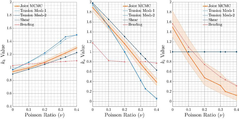
Figure 17 Joint MCMC correction coefficients dependent on Poisson’s ratio with uncertainty, compared to individual Tension, Shear, and Bending test results.
5 Conclusion
This study presents a Bayesian inverse method to calibrate lattice element models for accurate elastic behaviour. Due to their discrete and irregular structure, lattice models can represent only limited range of elastic deformations associated with Poisson ratio. Additionally, they posses non-uniform stress and displacement fields. To overcome this, we introduced correction coefficients into the discrete Timoshenko beam lattice model for axial, shear, and bending stiffness to improve its performance and to enable a wide range of lateral deformations. Irregular meshes based on Delaunay triangulation and Voronoi tessellation offer a good balance of homogeneity and isotropy, affecting the mechanical response and required corrections.
Using gPCE and MCMC, we efficiently identified stiffness correction coefficients across tensile, shear, and bending tests. Longitudinal and shear coefficients were consistently identifiable; bending stiffness could be only identified using bending test. The coefficients depend on mesh structure, geometry, and test type, indicating no universal set exists. With calibrated stiffness matrices, lattice models closely matched reference FEM displacement fields, validating the approach. Although the identification procedure must be repeated for different Poisson’s ratios, tensile tests conducted on two mesh resolutions demonstrate that the identified coefficients are mesh-independent and remain nearly identical across both meshes.
Lattice models, which are not calibrated with correction coefficients, struggle with alterations due to Poisson’s ratio variation and often fail to reproduce a uniform displacement field under uniform loading, indicating a deviation from the expected continuum elastic response. In contrast, our calibrated approach achieves better accuracy in simulating lateral strains induced by the Poisson effect and yields more uniform displacement fields. This provides advantages in modeling heterogeneous materials and establishes a robust foundation for non-linear fracture simulations. The Bayesian framework quantifies parameter uncertainties, enhancing model understanding and reliability for applications like concrete or rock analyses, where the one-time calibration effort is justified by improved simulation outcomes.
This framework bridges discrete and continuum modelling in elasticity and sets the basis for future work on non-linear fracture and crack propagation.
Author Contributions
Duje Pavić: Writing - Original Draft, Investigation, Visualization, Software. Noemi Friedman: Methodology. Hermann G Matthies: Original idea. Mijo Nikolić: Writing - Review & Editing, Supervision, Methodology, Investigation, Conceptualization.
Acknowledgments
This research has been supported by the project ‘Parameter estimation framework for fracture propagation problems under extreme mechanical loads’ (HRZZ-UIP-2020-02-6693), and the project ’Young Researchers’ Career Development Project – Training New Doctoral Students’ (DOK-NPOO-2023-10-8014), funded by the Croatian Science Foundation.
Additionally, the research has been supported by the projects KK.01.1.1.01.0003 (STIM-REI) and the project KK.01.1.1.02.0027, both funded by the European Union through the European Regional Development Fund – the Operational Programme Competitiveness and Cohesion 2014–2020.
The authors would like to acknowledge Andjelka Stanić for her contributions to the earlier stages of this research.
References
[1] A Ibrahimbegovic. (2009). Nonlinear solid mechanics: theoretical formulations and finite element solution methods (vol. 160). Heidelberg: Springer Science & Business Media.
[2] M Nikolić, E Karavelić, A Ibrahimbegovic and P Miščević. (2018). Lattice element models and their peculiarities. Archives of Computational Methods in Engineering 25(3), 753–784.
[3] A Lisjak and G Grasselli. (2014). A review of discrete modeling techniques for fracturing processes in discontinuous rock masses. Journal of Rock Mechanics and Geotechnical Engineering 6(4), 301–314.
[4] J Oliver, A E Huespe and P J Sánchez. (2006). A comparative study on finite elements for capturing strong discontinuities: E-FEM vs X-FEM. Computer Methods in Applied Mechanics and Engineering 195(37–40), 4732–4752.
[5] M Šodan, A Stanić and M Nikolić. (2024). Enhanced solid element model with embedded strong discontinuity for representation of mesoscale quasi-brittle failure. International Journal of Fracture 248(1), 1–25.
[6] E Karavelić, M Nikolić, A Ibrahimbegovic and A Kurtović. (2019). Concrete meso-scale model with full set of 3D failure modes with random distribution of aggregate and cement phase. Part I: Formulation and numerical implementation. Computer Methods in Applied Mechanics and Engineering 344, 1051–1072.
[7] A Hrennikoff. (1941). Solution of problems of elasticity by the framework method. Journal of Applied Mechanics 8(4), A169–A175.
[8] M Ostoja-Starzewski. (2002). Lattice models in micromechanics. Applied Mechanics Reviews 55(1), 35–60.
[9] E Schlangen and J G M Van Mier. (1992). Simple lattice model for numerical simulation of fracture of concrete materials and structures. Materials and Structures 25(9), 534–542.
[10] E Schlangen and E J Garboczi. (1996). New method for simulating fracture using an elastically uniform random geometry lattice. International Journal of Engineering Science 34(10), 1131–1144.
[11] G Cusatis, D Pelessone and A Mencarelli. (2011). Lattice Discrete Particle Model (LDPM) for failure behavior of concrete. I: Theory. Cement and Concrete Composites 33(9), 881–890.
[12] J E Bolander Jr and S Saito. (1998). Fracture analyses using spring networks with random geometry. Engineering Fracture Mechanics 61(5–6), 569–591.
[13] J E Bolander, J Eliáš, G Cusatis and K Nagai. (2021). Discrete mechanical models of concrete fracture. Engineering Fracture Mechanics 257, 108030.
[14] J Čarija, E Marenić, T Jarak and M Nikolić. (2024). Discrete lattice element model for fracture propagation with improved elastic response. Applied Sciences 14(3), 1287.
[15] M Nikolic, A Ibrahimbegovic and P Miscevic. (2015). Brittle and ductile failure of rocks: Embedded discontinuity approach for representing mode I and mode II failure mechanisms. International Journal for Numerical Methods in Engineering 102(8), 1507–1526.
[16] D Asahina, K Ito, J E Houseworth, J T Birkholzer and J E Bolander. (2015). Simulating the Poisson effect in lattice models of elastic continua. Computers and Geotechnics 70, 60–67.
[17] G F Zhao, Q Yin, A R Russell, Y Li, W Wu and Q Li. (2019). On the linear elastic responses of the 2D bonded discrete element model. International Journal for Numerical and Analytical Methods in Geomechanics 43(1), 166–182.
[18] L Vaiani, A E Uva and A Boccaccio. (2025). Optimal lattice spring models derived from triangular and tetrahedral meshes. International Journal of Mechanical Sciences 110442.
[19] D Xiu. (2010). Numerical methods for stochastic computations: a spectral method approach. Princeton: Princeton University Press.
[20] B V Rosić, A Kučerová, J Sýkora, O Pajonk, A Litvinenko and H G Matthies. (2013). Parameter identification in a probabilistic setting. Engineering Structures 50, 179–196.
[21] H G Matthies, E Zander, B V Rosić, A Litvinenko and O Pajonk. (2016). Inverse problems in a Bayesian setting. Computational Methods for Solids and Fluids: Multiscale Analysis, Probability Aspects and Model Reduction (245–286). Cham: Springer International Publishing.
[22] B Rosić, J Sýkora, O Pajonk, A Kučerová and H G Matthies. (2016). Comparison of numerical approaches to Bayesian updating. Computational Methods for Solids and Fluids: Multiscale Analysis, Probability Aspects and Model Reduction (427–461). Cham: Springer International Publishing.
[23] F Landi, F Marsili, N Friedman and P Croce. (2021). gPCE-based stochastic inverse methods: A benchmark study from a civil engineer’s perspective. Infrastructures 6(11), 158.
[24] N Friedman, C Zoccarato, E Zander and H G Matthies. (2021). A worked-out example of surrogate-based bayesian parameter and field identification methods. Bayesian Methods for the Analysis of Engineering Systems; J Chiachio Ruano, M Chiachio Ruano, S Sankararaman, Eds. Boca Raton: CRC Press.
[25] F Marsili, N Friedman, P Croce, P Formichi and F Landi. (2016). On Bayesian identification methods for the analysis of existing structures. Proceedings of the IABSE Congress Stockholm, Challenges in Design and Construction of an Innovative and Sustainable Built Environment, Stockholm, Sweden (21–23).
[26] Y Huang, C Shao, B Wu, J L Beck and H Li. (2019). State-of-the-art review on Bayesian inference in structural system identification and damage assessment. Advances in Structural Engineering 22(6), 1329–1351.
[27] M Å odan, A Urbanics, N Friedman, A Stanic and M Nikolić. (2025). Comparison of Machine Learning and gPC-based proxy solutions for an efficient Bayesian identification of fracture parameters. Computer Methods in Applied Mechanics and Engineering 436, 11768.
[28] W K Hastings. (1970). Monte Carlo sampling methods using Markov chains and their applications. Biometrika Volume 57, Issue 1, 97–109.
[29] A Saltelli, P Annoni, I Azzini, F Campolongo, M Ratto and S Tarantola. (2010). Variance based sensitivity analysis of model output. Design and estimator for the total sensitivity index. Computer Physics Communications 181(2), 259–270.
[30] I M Sobol. (2001). Global sensitivity indices for nonlinear mathematical models and their Monte Carlo estimates. Mathematics and Computers in Simulation 55(1–3), 271–280.
[31] M Nikolić. (2022). Discrete element model for the failure analysis of partially saturated porous media with propagating cracks represented with embedded strong discontinuities. Computer Methods in Applied Mechanics and Engineering 390, 114482.
[32] A Stanic, M Nikolic, N Friedman and H G Matthies. (2021). Parameter identification in dynamic crack propagation. ECCOMAS MSF 2021 – 5th International Conference on Multi-scale Computational Methods for Solids and Fluids.
[33] E Hadzalic, A Ibrahimbegovic and S Dolarevic. (2019). Theoretical formulation and seamless discrete approximation for localized failure of saturated poro-plastic structure interacting with reservoir. Computers & Structures 214, 73–93.
[34] E Hadzalic, A Ibrahimbegovic and M Nikolic. (2018). Failure mechanisms in coupled poro-plastic medium. Coupled Systems Mechanics 7, 43–59.
[35] E Hadzalic, A Ibrahimbegovic and S Dolarevic. (2020). 3D thermo-hydro-mechanical coupled discrete beam lattice model of saturated poro-plastic medium. Coupled Systems Mechanics 9(2), 125–145.
[36] H Rana and A Ibrahimbegovic. (2025). Fine-scale model of concrete composite for long-term cycling transient loads incorporating nonlinear hardening and softening effects. Composite Structures, 119649.
[37] H Rana and A Ibrahimbegovic. (2025). A hybrid physics-informed and data-driven approach for predicting the fatigue life of concrete using an energy-based fatigue model and machine learning. Computation 13(3), 61.
[38] D Xenos, D Grégoire, S Morel and P Grassl. (2015). Calibration of nonlocal models for tensile fracture in quasi-brittle heterogeneous materials. Journal of the Mechanics and Physics of Solids 82, 48–60.
[39] P J Green and R Sibson. (1978). Computing Dirichlet tessellations in the plane. The Computer Journal 21(2), 168–173.
[40] S P Timoshenko. (1921). LXVI. On the correction for shear of the differential equation for transverse vibrations of prismatic bars. The London, Edinburgh, and Dublin Philosophical Magazine and Journal of Science 41(245), 744–746.
[41] R L Taylor. (2014). FEAP, a finite element analysis program: Version 7.1 j user manual. Department of Civil and Environmental Engineering, University of California.
[42] E Zander and J Vondrejc. (2016). A MATLAB/Octave toolbox for stochastic Galerkin methods. Github, San Francisco, CA.
Biographies
Duje Pavić is a PhD student at the University of Split’s Faculty of Civil Engineering, Architecture and Geodesy, where he focuses on advanced discrete element modelling and Bayesian calibration techniques in computational mechanics. He earned his master’s degree in Civil Engineering from University of Split.

Noemi Friedman is a Senior Research Fellow and Lead Researcher at the AI Laboratory of HUN-REN SZTAKI (Institute for Computer Science and Control). She holds a degree in Structural Engineering from the Budapest University of Technology and Economics (BME) and a PhD in Civil Engineering from a joint program between ENS de Cachan (France) and BME. Her work focuses on big data analysis, predictable models based on physics and data, digital twinning, trustable AI methods, probabilistic, Bayesian methods, explainable AI, and uncertainty quantification for different engineering applications. She was recognized among the Top 15 awardees of the HTE “Top 50 Women in Artificial Intelligence in Hungary” program.

Hermann G Matthies is an emeritus professor in the Department of Computer Science at the Technische Universitaet Braunschweig. His research interests include scientific computing and computational engineering, in particular computational methods for inverse problems, uncertainty quantification, and coupled problems. He obtained his first degree from TU Berlin and his PhD at MIT.

Mijo Nikolić is an associate professor in the Department of Mechanics at the Faculty of Civil Engineering, Architecture and Geodesy, University of Split. His research focuses on civil engineering and computational mechanics, with an emphasis on the development of novel computational tools and models.
European Journal of Computational Mechanics, Vol. 34_3&4, 241–274
doi: 10.13052/ejcm2642-2085.34343
© 2026 River Publishers