Integrated Flood Hazard Assessment using GIS and 2D Hydraulic Modelling: A Case Study of Sanica River, Bosnia and Herzegovina

Nerma Lazović^* and Ajla Mulaomerović-Šeta

¹University of Sarajevo-Faculty of Civil Engineering, Patriotske lige 30, 71000 Sarajevo, Bosnia and Herzegovina
E-mail: nerma.lazovic@gf.unsa.ba
^∗Corresponding Author

Received 25 July 2025; Accepted 25 September 2025

Abstract

Flood extent maps (FEM) and flood hazard maps (FHM) serve as legal instruments for spatial planning, decision-making, strategic flood risk planning, and public awareness, supporting sustainable and safe land use along the river corridor. This study aims to improve existing FEM and create FHM for the Sanica river, prone to frequent flooding. The existing FEM were developed using a 1D HEC-RAS model under steady-flow conditions, applying a single uniform Manning roughness coefficient along the entire river reach. The study presents the first application of an unsteady 2D HEC-RAS model along Sanica river, integrating LiDAR-based topography and updated hydrological data to derive FEM and FEH for common return periods. The final 2D hydraulic model was selected through calibration of seven variants of the Manning roughness coefficient, three lumped and four distributed, with the optimal configuration identified based on three goodness-of-fit measures. The comparison of 1D and 2D FEM shows close agreement in morphologically confined canyon reaches, while significant differences occur in river sections with floodplain inundation and dominant 2D flow. These results indicate that model dimensionality can be selected based on reach-scale morphology, enabling the use of 1D models in canyon sections to reduce computational time, while applying 2D models only where complex flow dynamics are present within the Sanica river study area.

Keywords: Flood extent map, flood hazard maps, 2D hydraulic modelling, GIS, Manning’s coefficient, Sanica river.

1 Introduction

Floods are among the most frequent and destructive natural hazards worldwide, with increasingly severe socioeconomic and ecological consequences driven by rapid urbanization, land-use changes, and climate variability [1, 2]. In the context of Bosnia and Herzegovina (BIH), these global drivers are further exacerbated by the country’s geographical and climatic characteristics, the institutional complexity and fragmentation of the water management sector, and limited investments in preventive measures. The flood event in 2014, one of the most destructive floods that affected BIH and the region [3–6], clearly demonstrated the need for improved planning, inter-institutional coordination, and the application of advanced technical tools for flood protection. This event prompted a series of targeted actions implemented by the competent water management agencies in the subsequent years.

Creating flood extent maps (FEM) and flood hazard maps (FHM) for different return periods are particularly significant for planning of adequate flood protection. According to the Water Law of BIH, FEMs serve as a key regulatory instrument in spatial planning and in determining minimum construction setbacks. In accordance with the EU Floods Directive [7], FHMs provide detailed identification of areas potentially exposed to flooding, including assessments of water depth, extent, and flow dynamics. These maps form the basis for both strategic and operational flood risk management [8–10] supporting the development of protection plans, informed spatial decision-making, and increasing public awareness of flood hazards [11, 12].

The application of hydraulic modelling is a fundamental component in the development of FHM [13], as it enables a quantitative assessment of the interaction between watercourses, surrounding terrain, and hydraulic processes during extreme hydrological events. Contemporary hydraulic models include various approaches and levels of complexity [14, 15] from simplified one-dimensional (1D) models [16, 17], through combined 1D/2D approaches [18], to fully two-dimensional (2D) models that provide detailed representation of horizontal water movement over complex terrain [19–21].

Although each model type has its specific purpose depending on the analysis objective and data availability, 2D models have proven to be reliable and effective tool for flood inundation modelling [22–24]. Their ability to continuously describe spatial patterns of flooding, as well as distributed flow velocities and water depths, significantly enhances the accuracy of identifying high-hazard risk zones.

The reliability of hydraulic model outputs is primarily governed by the accuracy of input data and the adequacy of the selected model framework. The accuracy of hydrological inputs, particularly flood quantile estimates, depends on both the length of the available discharge time series and the appropriateness of the assumed probability distribution. Furthermore, accurate terrain representation is a fundamental requirement for flood modelling. LiDAR-derived Digital Terrain Models (DTMs) ensure high-resolution topographic detail, which is essential for reliable flood extent delineation [8, 25–30]. With respect to hydraulic parameters, the selection of Manning’s roughness coefficient remains a key source of uncertainty due to its substantial impact on simulated flow conditions and water levels [31–34].

In this study, FEM and FHM were developed for the flood-prone Sanica river. Existing FEMs produced using 1D steady-flow modelling are of limited applicability in morphologically complex reaches with significant inundation and dominant 2D flow, where 2D hydraulic modelling is required. Moreover, the hydrological input in existing FEM was based on a relatively short 24-year annual maximum series, not accounting for recent extreme events. To address these limitations, the present study applies advanced 2D unsteady-flow modelling supported by a high-resolution 1 m LiDAR-derived DTM. The hydrological analysis was updated to include extreme events recorded up to 2023. Hydraulic simulations were performed using HEC-RAS 2D hydraulic model, complemented by a sensitivity analysis of Manning’s roughness coefficient based on land-use categories. Free QGIS software is used for data processing, FEM creation and results visualization. The resulting FEM and FHM provide improved spatial accuracy in reaches with extensive inundation.

2 Materials and Methods

2.1 Study Area

The Sanica river, located in western BIH, is a 22 km long tributary of the Sana river with a catchment area of 211 km², belonging to the Black Sea basin (Figure 1). It originates from a spring zone at the foot of the Grmeč massif at 225 m a.s.l., at the coordinates 44${}_{}{}^{\circ }17_{}^{\prime }{49}^{\prime \prime }$ N and ${16}^{\circ }{8}^{\prime }{11}^{\prime \prime }$ E and its confluence with the Sana is at 177 m a.s.l.

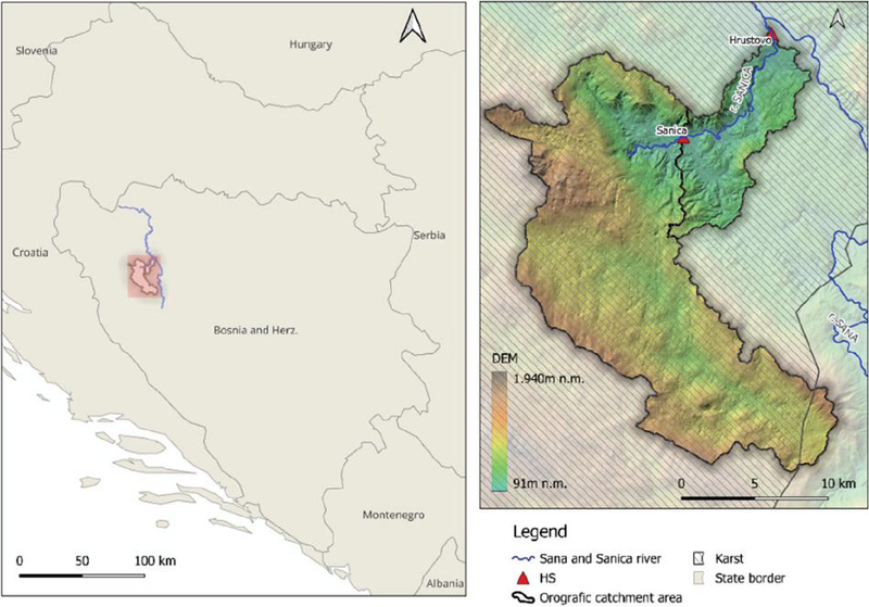
Figure 1 Representation of the orographic boundary of the catchment and karst in the wider area of hydrological stations on the Sanica river (left) and terrain elevation (right).

The spring zone includes three sources, the most significant being a cave spring connected to the Gornja Sanica basin. Between Sanica Donja and Saleševići, it forms a canyon valley exceeding 100 m in depth, while the final section runs parallel to the Sana. The river is characterized by numerous waterfalls along its course.

2.2 Hydrological Data

Hydrological station (HS) Hrustovo began operating in 1966. Until 1990, data were collected once a day. In 2005, an automatic station was installed, with hourly timestep resolution. Data from 1990 until 2005 is missing, since the station was not in operation. Total recording length is 44 years. For flood quantile estimation statistical analysis of annual maxima series (AMS) is used. Discharge data at HS Sanica has been measured since 2018 and is therefore not suitable for statistical analysis of AMS. Flood quantiles at HS Sanica is determined through linear regression with the HS Hrustovo (coefficient of correlation for AMS data $r^2=0.995$, Figure 2).

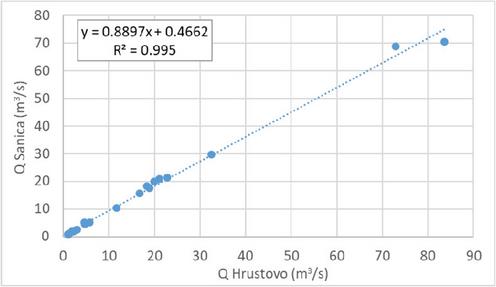
Figure 2 Simultaneous discharge data on HS Hrustovo (x-axis) and HS Sanica (y-axis).

Statistical tests showed that AMS at HS Hrustovo is independent (Mann-Kendall test) and homogeneous in mean value (Mann-Whitney, Kruskal-Wallis (KW), Student’s t-test, Z test) and variance (Fisher’s F test, Levene test) at the 5% significance level. According to single Grubbs-Beck test (SGBT), one low outlier is confirmed, while multiple Grubs-Beck test (MGBT) revealed seven potential influential low flows (PILF values) (Figure 1). Statistical parameters of AMS for HS Hrustovo (original and log sample) are shown in Table 1.

Table 1 Statistical parameters of AMS (from existing documents) and updated series (original and log transformed) at HS Hrustovo (1967–1990 and 2005–2023)

Statistical	1967–1990	1967–1990,	1967–1990,	Original	Log
Parameter	[35]	2005–2016 [36]	2005–2016 [37]	Data	Data
Mean value (m3/s)	131	131	132	133	2.111
Standard dev (m3/s)	30.5	31.7	31.9	30.2	0.1129
Cs	$-$0.23	$-$0.23	$-$0.3	$-$0.40	$-$1.3583
Cv	0.23	0.24	0.24	0.23	0.0535

For quantile estimation 3-parametric probabilistic distribution functions (pdf) are used, employing 3-parameter estimation methods:

• P3, LP3, with method-of-moments (MOM) (common in hydrological analysis in BIH)

• P3, GLO and GEV with L-moments method (LMOM)

• LP3 with Expected Moment Algorithm (EMA) according to Bulletin 17C (B17C) procedure

Table 2 Quantile estimates Q(T) (m³/s) at HS Hrustovo according to different documentation, distribution function, parameter method estimation and PT

T	1967–1990 [36]	1967–1990, 2005–2016 [37]	1967–1990, 2005–2016 [38]	MOM		LMOM			LP3 EMA (B17C)
*			P3, MOM	P3	LP3	GLO	P3	GEV	PT 200	PT 250	Omit gap
20	188	191	181	179	176	178	177	177	179	180	180
100	215	222	199	194	184	199	191	187	202	205	205
500	240	250	212	206	187	215	200	192	225	228	229
∗Unknown pdf and estimation method

In cases of complete data with no PILF values, the EMA algorithm is the same as MOM, while adjusting it otherwise. The 14 years of missing data are described by perception threshold (PT) (assuming AMS is less than PT in missing data years), while one analysis neglected missing data (the series was considered complete). Results of all applied pdf and estimation method are presented in Table 2. P3 (MOM) and LP3 (B17C neglecting missing data) are shown in Figure 3. Statistical analysis estimates the peak of the hydrograph while its shape is unknown. In order to define the shape of the hydrograph, the two largest events with peak (Q_max) of 202 m³/s (16.05.2014) and 193 m³/s (14.04.1984) were analysed (Figure 4 top). Dividing each hydrograph with its peak, two dimensionless hydrographs were derived (Figure 4 bottom). As the shape of the hydrograph from 1984 resembles the flood waves of previous studies [36, 37], it was chosen as relevant for return period hydrograph construction. Due to limited data at HS Sanica, input flood hydrographs of 20, 100 and 500 return period was estimated based on the correlation with HS Hrustovo (Figure 5).

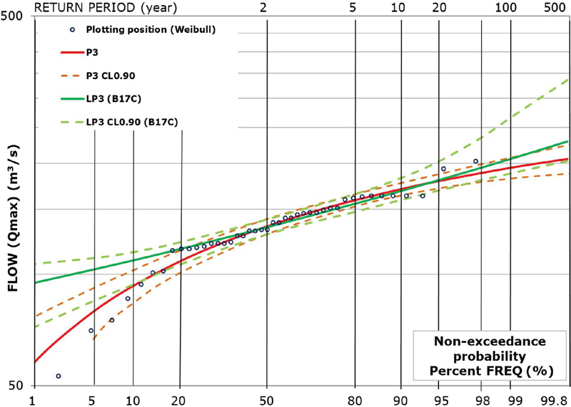
Figure 3 Flood quantile estimation using LP3 (EMA) and P3 (LMOM) with Weibull plotting position and 90% confidence limit (CL).

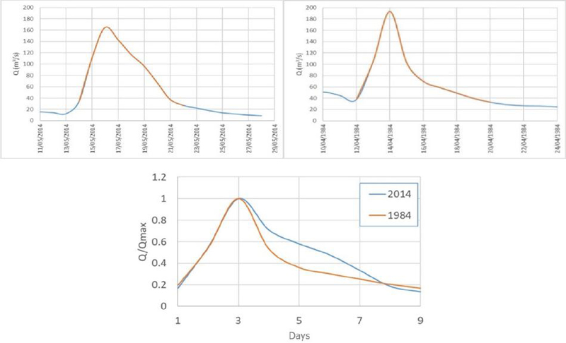
Figure 4 Flood hydrographs from the two extreme events: 2014 and 1984 (top) and two dimensionless flood hydrographs (bottom).

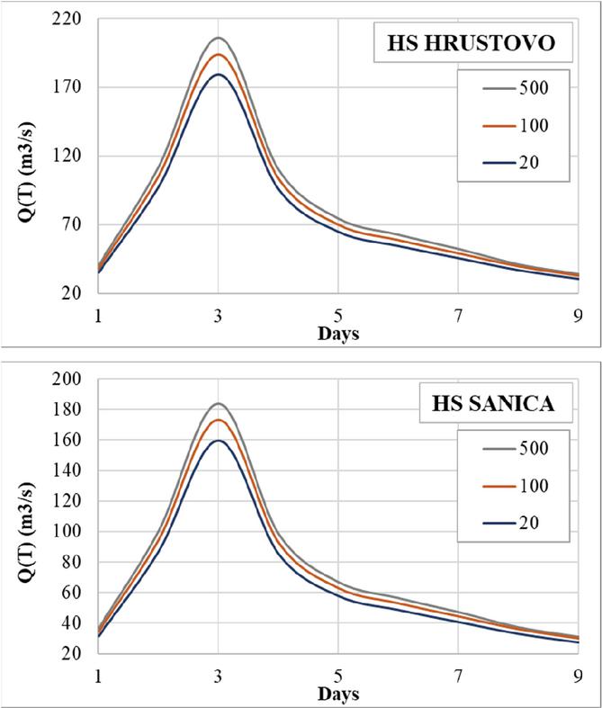
Figure 5 Flood hydrographs at HS Hrustovo (top) and HS Sanica (bottom).

2.3 HEC-RAS 2D model

2D hydraulic modelling represents a central component of the flood hazard assessment, as it enables spatially explicit simulation of flow dynamics and inundation processes. In this study, a detailed 2D hydraulic model was developed using HEC-RAS 2D version 6.3.1, a commercial software package developed by the U.S. Army Corps of Engineers Centre. The software provides robust numerical capabilities for solving shallow water flow and simulating flood propagation across complex terrains.

The hydraulic computations in HEC-RAS 2D are based on the 2D shallow water equations (Saint-Venant equations), which describe the conservation of mass and momentum for free-surface flow [38]. These equations are widely used for flood modelling applications due to their suitability for simulating non-uniform, unsteady, and rapidly varying flows [27, 39, 40].

The numerical scheme employed in HEC-RAS 2D relies on a finite-volume method with an implicit solution approach, enabling stable computations even under highly variable flow conditions. The governing equations and the numerical aspects of the scheme used can be found in full detail in [41] and it has been extended to 2D unstructured meshes in [38].

The hydraulic model of the Sanica river covers its entire length, from the source to the confluence with the Sana river.

The input data required for the hydraulic model setup included:

• Geometric data of the riverbed and inundation area.

• Hydrological data on characteristic flood hydrographs (Figure 5).

• Hydrological data on flood waves from December 2022 and May 2023, recorded at the HS Hrustovo gauging stations, used for model calibration and verification (Figure 7).

The geodetic basis consisted of LiDAR-derived DTM with a spatial accuracy of 1 m, complemented by digital orthophoto maps and photographic documentation of the flood events from December 2022 and May 2023.

The mesh is defined within a preselected 2D Flow Area polygon. For the hydraulic model of the Sanica river, the computational mesh consists of 8336 cells. To achieve a more accurate terrain representation, the cell size in the inundation area is $30\times 30$ m, while in the riverbed area it is $10\times 10$ m (Figure 6).

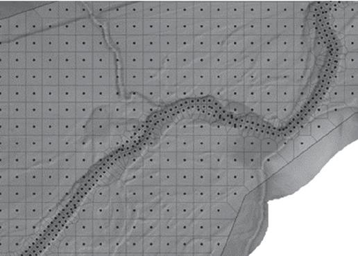
Figure 6 Definition of the computational mesh of the 2D hydraulic model of the Sanica river.

After defining the computational mesh, particular attention was given to the selection of Manning’s roughness coefficients. Seven scenarios were generated with different Manning coefficient values, ranging from a single literature-based estimates (lumped model) to values derived for every pixel based on the analysis of digital orthophoto maps and satellite imagery (e.g., CORINE Land Cover, Google Earth) (distributed model).

The spatial domain of the 2D model was classified into distinct land use categories, with each category assigned an appropriate Manning coefficient based on literature sources. The final values of the Manning coefficients were determined through model calibration.

2.4 Calibration and Verification of the Hydraulic Model

For the calibration of the 2D hydraulic model, flood wave data from December 2022 was used, while the model verification was based on data from May 2023 recorded at the Hrustovo and Sanica gauging stations. The calibration parameter was the Manning roughness coefficient, one of the most critical parameters in hydrodynamic flood simulations. The Manning’s roughness coefficient varies with land use and soil/vegetation conditions, and HEC-RAS allows these variations to be represented by assigning region-specific roughness values through dedicated spatial layers [41].

Calibration was carried out by performing numerical simulations of high-flow conditions on the Sanica river for December 2022. The simulated water levels at HS Hrustovo were compared with the observed water levels. In each simulation, different Manning coefficient values were applied. The final coefficients were adopted for the case showing the smallest deviation between simulated and observed values.

Models M1, M2 and M3 applied a uniform Manning coefficient across the entire computational domain (lumped model). The values were selected based on the estimated roughness of the channels, with Model 1 representing the highest resistances and Model 3 the lowest. A roughness value of 0.6 was assigned to Model 1, corresponding to a gravel-bed channel with coarse material and floodplain areas covered by shrubs and trees. Model 2 represents a gravel-bed channel with finer sediment and floodplains covered by grass and sparse shrubs, while Model 3 correspond to a gravel-bed channel without vegetation and floodplain areas characterized by pastureland.

In Models 4–7, the computational domain was divided into zones with different Manning coefficients (distributed model), which correspond to recommended values from the literature for individual land covers (Table 3).

Table 3 Model calibration: Manning roughness coefficients in the 2D model

Land Use Type	M1	M2	M3	M4	M5	M6	M7
Riverbed	0.06	0.05	0.04	0.035	0.035	0.045	0.03
Forest	0.06	0.05	0.04	0.12	0.25	0.30	0.30
Grass	0.06	0.05	0.04	0.045	0.06	0.10	0.10
Road	0.06	0.05	0.04	0.03	0.04	0.04	0.04

The selection of the Manning’s roughness parameter was based on the goodness-of-fit measure (Table 4). The calculations were performed in the R programming environment using the hydroGOF package which provides the equations for all applied performance metrics [42]. The best goodness-of-fit measure is achieved in model 6 (two out of three applied measures), so the parameters of model 6 were adopted for further hydraulic analysis.

Table 4 Goodness-of-fit measure obtained in calibration and verification for water level values at HS Hrustovo

	Calibration							Verification
Measure	M1	M2	M3	M4	M5	M6	M7	M6
Nash–Sutcliffe Efficiency (NSE)	$-$3.058	0.588	$-$0.889	$-$4.620	$-$4.495	0.550	$-$10.748	0.890
Mean Absolute Error (MAE)	0.282	0.077	0.192	0.337	0.332	0.078	0.487	0.150
Root Mean Square Error (RMSE)	0.288	0.092	0.197	0.339	0.335	0.092	0.491	0.180
Bolded values represent best fit.

The next step was verification of model 6 on HS Hrustovo for the observed flood wave from May 2023 (Figure 7 right). The verification process results in slightly lower goodness-of-fit measures. Despite this reduction, the overall model performance remains similar to calibration values and outperforms goodness-of-fit values for other models (Table 4).

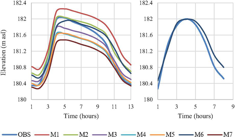
Figure 7 Model calibration M1-M7 (left) and verification M6 (right) at HS Hrustovo.

2.5 Flood Zone Mapping

In practical FHMs, the most used formula for quantitative hazard classification is based on the combination of water depth (h) and flow velocity (v). The standard and most widely accepted formula – used in the United Kingdom (DEFRA/Environment Agency) [11, 43], EU projects (e.g., FLOODsite) [45], and adopted in many methodologies in BIH [45, 46] – is:

$$O=h\times (v+0.5)$$

(1)

where $O$ is hazard, $h$ is flooding depth (m), $v$ is flow velocity (m/s), and 0.5 is a correction constant for velocity.

FHM can be classified into four categories:

• Low hazard – negligible threat (hazard value up to 0.75)

• Moderate hazard – specific vulnerable groups are at risk (children, the elderly, the ill, non-swimmers), with hazard values between 0.75 and 1.5

• High hazard – the majority of the population is at risk (hazard values between 1.5 and 2.5)

• Extreme hazard – all people in the flood-prone area are at risk (hazard values above 2.5).

The development of FHMs was conducted in QGIS based on raster datasets of flow velocities and water depths generated through 2D hydraulic modelling in HEC-RAS and subsequently processed using Equation (1). The selected horizontal resolution of FHM (and consequently FEM) is $10\times 10$ m, with vertical accuracy up to 10 cm. FHM ($10\times 10$ m) provides a finer spatial representation for visualization and planning purposes, while computational mesh ($30\times 30$ m) defines the numerical resolution of the hydraulic model, balancing accuracy and computational efficiency. The apparent higher map resolution does not increase the intrinsic accuracy, which remains limited by the coarser model grid.

3 Results

FEM and FHM were developed using 2D HEC-RAS unsteady-flow simulations for the selected return periods. A comparative representation of the 100-year FEM obtained from the existing 1D steady-flow model (the only one available in digital form) and the 2D unsteady-flow model developed in this study is shown in Figure 8. Based on the velocity and depth raster data (not shown here due to space limitations), FHM for return periods $T=20$ (Figure 10), $T=100$ (Figure 10), and $T=500$ (Figure 11) were generated using Equation (1) and the previously described classification. Figures 10–11 present the FEM at a coarser scale, while selected sections of the FHM are shown at a finer scale to ensure better visibility.

The QGIS toolbox is used to intersect FHM with land use data (CORINE Land Cover 2018 [47]). As a result, the areas exposed to different flood hazards were identified. The results, summarized in Table 5, indicate that agricultural land is the most vulnerable to flood hazards, as large portions of the inundation zones overlap with croplands and grasslands. In contrast, the exposure of residential areas is relatively low.

The flooded area was derived from FEM for return periods of $T=20,100$, and 500 years and is presented in Figure 12, indicating a near-linear increase in inundation extent with increasing flow.

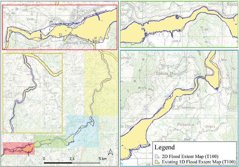
Figure 8 A comparative representation of the 100-year FEM obtained from the existing 1D steady-flow model and the 2D unsteady-flow model.

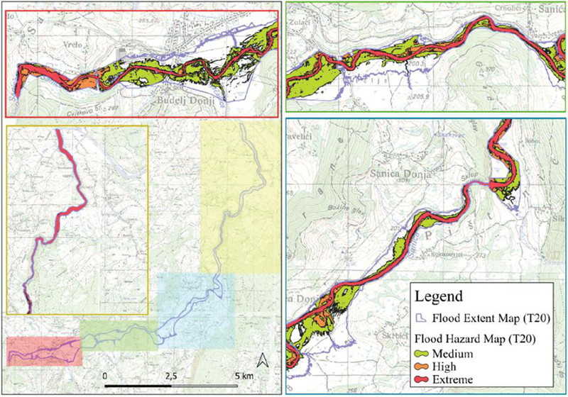
Figure 9 FHM for the 20-year return period flood for Sanica river.

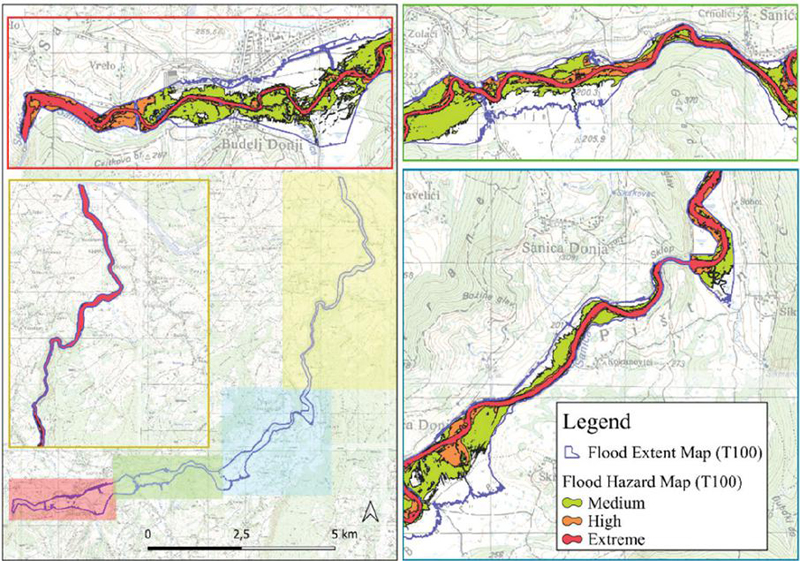
Figure 10 FHM for the 100-year return period flood for Sanica river.

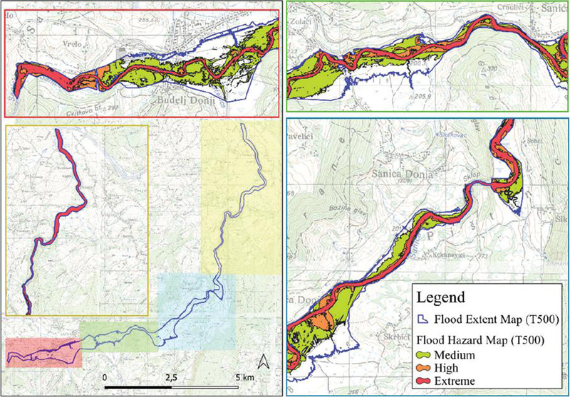
Figure 11 FHM for the 500-year return period flood for Sanica river.

Table 5 Areas (ha) exposed to flood hazard for different return period flood

Land Cover (CLC 2018)	Flood Hazard	T20	T100	T500
Artificial surfaces (settlements)	Extreme	0.70	0.76	0.82
	High	0.87	1.00	1.10
	Medium	4.92	5.51	5.95
Agricultural areas	Extreme	66.41	69.67	72.42
	High	28.11	31.35	33.90
	Medium	68.68	75.93	80.58
Forest and semi-natural areas	Extreme	28.70	29.30	29.68
	High	3.09	3.13	3.16
	Medium	3.11	3.16	3.25

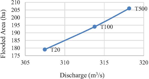
Figure 12 Flooded area with an increase in discharge.

4 Discussion

There are several documents that analyse the quantiles at HS Hrustovo processing different periods. These analyses were conducted in varying degrees of detail, from [35, 36] where no outliers test applied, to [37] which is significantly more detailed. Regardless of considering a different period, the statistical parameters are close. It is not possible to comment the difference in the quantile values in [35, 36] compared to the more recent analyses [37], since the former do not specify pdf or the parameter estimation method, which could significantly affect the results [48, 49]. It can be noted that the 500-year quantiles defined in [35, 36] fall outside the 90% Confidence Interval limit of P3 function.

In this study, in addition to the P3 function, other pdfs were used to examine the influence of PILF on the right end of the distribution, so the GEV distribution was also chosen, confirmed as insensitive to existence PILF values [50]. Since there are no significant differences in quantiles, P3 was adopted with the MOM parameter evaluation method, as in [37], which is mostly used in BIH. Due to the relatively small value of Cs (uncommon for AMS in this area [51]), the difference in the 100-year and 500-year quantile is small. The skew coefficient (C_s) of the log sample is also close to the usual limit values of AMS in USA [52]. Negative C_s can be explained by attenuation influences attributable to floodplains [53, 54] or as the result of karst area through the possible limited capacities of the source zones [55, 56], the variability of the catchment area [57, 58] or the retention of water in karst system [59, 60].

Due to limited data at HS Sanica, flood hydrographs for the 20-, 100-, and 500-year return periods were estimated from HS Hrustovo. This introduces uncertainties, partly from the method itself and partly from significant wave transformation caused by upstream overflow, which may delay flood volumes and affect the correlation. These uncertainties should be considered in future river regulation, as interventions could increase downstream flooding, including in areas previously unaffected. On the other hand, potential climate change is also one of the possible causes of changes in FEM and FHM. Many analyses conducted at the global level have shown that changes in flows can be expected, however, not all agree on the direction and magnitude of the change [61–64].

Given the substantial influence of the Manning roughness coefficient on the reliability of the 2D HEC-RAS model [32, 65]—as it governs flow resistance and thereby affects velocity distribution, water levels, and flood extent—particular attention was devoted to its accurate selection in this study. Urbanization reduces Manning’s coefficient by increasing flow velocities and peak discharges, thereby elevating flood hazard, while vegetation or wetlands increase Manning’s coefficient, slowing runoff and mitigating flood impacts. These effects influence flood depth, extent, and timing across the catchment.

The comparative analysis of 1D (existing model) and 2D hydraulic modelling results for the 100-year flood extent along the Sanica river highlights a strong dependence of model performance on channel morphology. In the upper reach, where the channel widens and extensive overbank flow occurs, the 2D model more accurately captures complex, multidirectional flow patterns and the interaction between the main channel and the floodplain. Although differences in the flooded areas for the 100-year return period between the existing 1D and 2D models are small, notable discrepancies in FEM-derived flood lines are observed in urban zones and valleys. In the middle and lower reaches, FEMs are in close agreement between the 1D and 2D outputs. This can be explained by the canyon-type channel, where flow is predominantly 1D. These findings indicate that 1D modelling is sufficient in hydraulically simple, channelized sections with negligible lateral flow, whereas 2D modelling is preferable in areas with overbank flooding and spatially variable flow conditions. Recent studies [66, 67] further demonstrate that combined 1D/2D HEC-RAS models outperform standalone approaches, particularly in rivers with contrasting morphological characteristics (such as transitions from canyon segments to wide floodplains, like Sanica river) saving significant computational time. A near-linear correlation between flooded area and discharge at Sanica river is consistent with the findings of [22].

Comparison of the FHM for T20, T100, and T500 events highlight the vulnerability of low-lying agricultural and urban areas. These results confirm that high-resolution 2D hydraulic modelling is essential for identifying priority zones for flood risk management and for informing spatial planning, non-structural measures, and mitigation strategies in accordance with BIH and EU guidelines.

The results in Table 5 indicate differences in the spatial extent of flood hazard across land use categories (CLC 2018) and flood return periods (T20, T100, T500). Urban areas (artificial surfaces) show a small but stable increase in high and extreme risk areas (e.g., extreme risk rises from 0.70 ha to 0.82 ha), highlighting the importance of flood hazard planning due to the high exposure of people and infrastructure. Agricultural areas dominate the total flood hazard, with extreme risk ranging from 66.41 ha (T20) to 72.42 ha (T500), reflecting their location in alluvial plains prone to flooding. Forested and semi-natural areas exhibit lower hazard values with slight increases up to T500, as these areas provide natural flood attenuation, though some sections remain vulnerable. All land use categories show a consistent expansion of flood-prone areas with increasing return periods. These findings emphasize the importance of detailed FHM as non-structural measures for flood management, in line with BIH and EU legislation, for guiding construction, prioritizing protection, and planning preventive actions.

5 Conclusion

The Sanica river is characterized by frequent flooding, highlighting the importance of creating FEM and FHM in accordance with the water legislation of BIH and the EU Floods Directive. FEM represent a legally mandated element for defining construction conditions within the river corridor in BIH, while FHM serve as a key non-structural tool for managing flood risk.

The reliability of FEM and FHM depends on the accuracy of hydrological and morphological input data, as well as the choice of an appropriate model and its parameters. Considering the ongoing impacts of climate change, land-use changes (urbanization, deforestation) and the construction of structural flood protection measures (regulations, bank protections, retention structures), continuous updating of FEM and FHM is essential to ensure reliable flood risk assessments.

This study confirms the existence of differences between inundation extents produced by 1D and 2D hydraulic models. Based on the findings, it is recommended that 2D modelling be applied in river sections with wider floodplains and increased potential for overbank flow, whereas 1D modelling may still be suitable for confined, canyon-like segments of the channel.

The main limitations of this study are the lack of detailed local channel features (e.g., bridges) and limited calibration data, highlighting the need for additional cross-sectional measurements and temporary hydrological monitoring. The limitation of the presented FEM and FHM is that the influence of the confluence of the Sana and Sanica rivers was not considered during the numerical modelling, which can certainly be a topic for future research. Future research should investigate also climate change effects on flood magnitudes and assess potential hydraulic impacts of planned flood protection structures in the upper Sanica river, particularly regarding downstream flows.

Acknowledgements

The authors gratefully acknowledge the Federal Ministry of Education and Science of Bosnia and Herzegovina for supporting this research, and the Sava River Basin Agency for providing the LiDAR and hydrological data, which were necessary for conducting this research. We also extend our sincere thanks to the reviewers of this paper, whose constructive comments and valuable suggestions have significantly improved the quality of the manuscript.

References

[1] J Rentschler, M Salhab and B A Jafino, (2022). Flood exposure and poverty in 188 countries. Nat Commun, 13(1), 3527. doi: 10.1038/s41467-022-30727-4

[2] Z W Kundzewicz et al. (2014). Flood risk and climate change: global and regional perspectives. Hydrological Sciences Journal, 59(1), 1–28. doi: 10.1080/02626667.2013.857411

[3] J Plavsic, D Vladiković, and J Despotovic, (2014). Floods in the Sava river basin in May 2014. Proceedings of the Mediterranean meeting on monitoring, modelling and early warning of extreme events triggered by heavy rainfalls, Cosenza, Italy.

[4] L Stadtherr, D Coumou, V Petoukhov, S Petri and S Rahmstorf. (2016). Record Balkan floods of 2014 linked to planetary wave resonance. Science Advances, 2(4), p. e1501428. doi: 10.1126/sciadv.1501428

[5] A Vidmar et al. (2016). The Bosna river floods in May 2014. Natural Hazards and Earth System Sciences, 16(10), 2235–2246. doi: 10.5194/nhess-16-2235-2016

[6] E Haumont. (2015). Available: https://publications.iom.int/es/system/files/pdf/state\_environmental\_migration\_2014\_0\_0.pdf\#page=187

[7] R Smith. (2015). Directive 2008/94/EC of the European Parliament and of the Council of 22 October 2008. Core EU Legislation. London: Macmillan Education, 423–426. doi: 10.1007/978-1-137-54482-7_44

[8] L M Crenganis, C I Pricop, M Diac, A-M Olteanu-Raimond and A-M Loghin. (2025). Flood risk prediction and management by integrating GIS and HEC-RAS 2D hydraulic modelling: a case study of Ungheni, Iasi County, Romania. Water, 17(20), 2959. doi.org/10.3390/w17202959

[9] H D Skilodimou, G D Bathrellos and D E Alexakis. (2021). Flood hazard assessment mapping in burned and urban areas. Sustainability, 13(8), 4455. doi: 10.3390/su13084455

[10] S N Sahoo and P Sreeja. (2017). Development of flood inundation maps and quantification of flood risk in an urban catchment of Brahmaputra river. ASCE-ASME Journal of Risk and Uncertainty in Engineering Systems, Part A: Civil Engineering, 3(1), A4015001. doi: 10.1061/AJRUA6.0000822

[11] R B Mudashiru, N Sabtu, I Abustan and W Balogun. (2021). Flood hazard mapping methods: a review. Journal of Hydrology, 603, 126846. doi: 10.1016/j.jhydrol.2021.126846

[12] A Maranzoni, M D’Oria and C Rizzo. (2023). Quantitative flood hazard assessment methods: a review. Journal of Flood Risk Management, 16(1), e12855. doi: 10.1111/jfr3.12855

[13] V Kumar, K Sharma, T Caloiero, D Mehta and K Singh. (2023). Comprehensive overview of flood modeling approaches: a review of recent advances. Hydrology, 10, 141. doi: 10.3390/hydrology10070141

[14] U C Nkwunonwo, M Whitworth and B Baily. (2020). A review of the current status of flood modelling for urban flood risk management in the developing countries. Scientific African, 7, e00269. doi: 10.1016/j.sciaf.2020.e00269

[15] P D Bates. (2004). Remote sensing and flood inundation modelling. Hydrological Processes, 18(13), 2593–2597. doi: 10.1002/hyp.5649

[16] V Demir and O Kisi. (2016). Flood hazard mapping by using geographic information system and hydraulic model: Mert river, Samsun, Turkey. Advances in Meteorology, 2016(1), 4891015. doi: 10.1155/2016/4891015

[17] J-M Tanguy and B Zhang. (2003). Propagation de crue en milieu urbain: REM²U: un outil 1D maillé aux éléments finis. European Journal of Computational Mechanics, 297–316.

[18] Q Qian, D J Edwards, Y Zhang and L Haselbach. (2024). Improving flood inundation mapping accuracy using HEC-RAS modeling: a case study of the Neches river tidal floodplain in Texas. Journal of Hydrologic Engineering, 29(4), 05024011. doi: 10.1061/JHYEFF.HEENG-6037

[19] M Gharbi, A Soualmia, D Dartus and L Masbernat. (2016). Comparison of 1D and 2D hydraulic models for floods simulation on the Medjerda River in Tunisia. J Mater Environ Sci, 7(8) 3017-3026.

[20] M Villazón, L Timbe and P Willems. (2013). Comparative analysis of 1-D river flow models applied in a quasi 2-D approach for floodplain inundation prediction. Maskana, 4(1), 107–126. doi: 10.18537/mskn.04.01.08

[21] T Faure, T Quach, J Joannette, M-H Briand and É NcNeil. (2003). Propagation d’onde de rupture de barrages et de crue: Applications de modélisation numérique 2D. European Journal of Computational Mechanics, 345–360.

[22] K Vashist and K K Singh. (2023). HEC-RAS 2D modeling for flood inundation mapping: a case study of the Krishna River Basin. Water Practice and Technology, 18(4), 831–844. doi: 10.2166/wpt.2023.048

[23] M Vojtek, A Petroselli, J Vojteková and S Asgharinia. (2019). Flood inundation mapping in small and ungauged basins: sensitivity analysis using the EBA4SUB and HEC-RAS modeling approach. Hydrology Research, 50(4), 1002–1019. doi: 10.2166/nh.2019.163

[24] Z Naiji, O Mostafa, N Amarjouf and H Rezqi. (2021). Application of two-dimensional hydraulic modelling in flood risk mapping. A case of the urban area of Zaio, Morocco. Geocarto International, 36(2), 180–196. doi: 10.1080/10106049.2019.1597389

[25] M Mihu-Pintile et al. (2019). Using high-density LiDAR data and 2D streamflow hydraulic modeling to improve urban flood hazard maps: a HEC-RAS multi-scenario approach. Water, 11(9), 1832.

[26] D L Ciurte et al. (2023). Integrating LiDAR data, 2D HEC-RAS modeling and remote sensing to develop flood hazard maps downstream of a large reservoir in the inner eastern Carpathians. Carpathian Journal of Earth and Environmental Sciences, 18(1), 149–169. DOI:10.26471/cjees/2023/018/248

[27] A Adane and B Abate. (2022). River modeling for flood inundation map predictions using 2D-HEC-RAS hydraulic modeling with integration of GIS. ASEAN Engineering Journal, 12(1), 9–15. doi: 10.11113/aej.v12.16483

[28] Y Z Kaya and F Üneş. (2025). Comparison of three different satellite data on 2D flood modeling using HEC-RAS (5_0_7) software and investigating the improvement ability of the RAS Mapper tool. Journal of Flood Risk Management, 18(1), e13046. doi: 10.1111/jfr3.13046

[29] P Gangani, N K Mangukiya, D J Mehta, N Muttil and U Rathnayake. (2023). Evaluating the efficacy of different DEMs for application in flood frequency and risk mapping of the Indian Coastal River Basin. Climate, 11(5), 114. doi: 10.3390/cli11050114

[30] B F Sanders. (2007). Evaluation of on-line DEMs for flood inundation modeling. Advances in Water Resources, 30(8), 1831–1843. doi: 10.1016/j.advwatres.2007.02.005

[31] S Kechida, F Laouacheria and L Zeghadnia. (2024). Assessment of the combined effects of Manning roughness and DEM resolution for the water surface elevation prediction using the HEC-RAS model: a case study of Moudjar River in the Northeast of Algeria. Model. Earth Syst. Environ, 10(1), 957–967. doi: 10.1007/s40808-023-01821-3

[32] I T C e Silva, H A Santos, L C O Pereira and K S do Nascimento. (2024). Global sensitivity analysis in flood mapping using HEC-RAS 2D: effects of the floodplain Manning coefficient for a dam-break case. RBRH, 29(e38). doi: 10.1590/2318-0331.292420240032

[33] G Papaioannou, V Markogianni, A Loukas and E Dimitriou. (2022). Remote sensing methodology for roughness estimation in ungauged streams for different hydraulic/hydrodynamic modeling approaches. Water, 14(7), 1076. doi: 10.3390/w14071076

[34] K Shahverdi and H Talebmorad. (2023). Automating HEC-RAS and linking with particle swarm optimizer to calibrate Manning’s roughness coefficient. Water Resour Manage, 37(2), 975–993. doi: 10.1007/s11269-022-03422-8

[35] Sava River Basin Agency. (2009). HIS Una: Hydrological information system of the Una River Basin. Sava River Basin Agency.

[36] Sava River Basin Agency. (2017). HIS Una: Hydrological information system of the Una River Basin. Sava River Basin Agency.

[37] Western Balkans Investment Framework – Infrastructure Project Support Facility (IPF5). (2018). Flood hazard and risk maps in Bosnia and Herzegovina – Hydrology (Technical assistance report). Western Balkans Investment Framework.

[38] I Echeverribar, M Morales-Hernández, P Brufau and P García-Navarro. (2019). 2D numerical simulation of unsteady flows for large scale floods prediction in real time. Advances in Water Resources, 134, 103444. doi: 10.1016/j.advwatres.2019.103444

[39] V A Rangari, N V Umamahesh and C M Bhatt. (2019). Assessment of inundation risk in urban floods using HEC RAS 2D. Model Earth Syst Environ, 5(4), 1839–1851. doi: 10.1007/s40808-019-00641-8

[40] N Kumar, M Kumar, A Sherring, S Suryavanshi, A Ahmad and D Lal. (2020). Applicability of HEC-RAS 2D and GFMS for flood extent mapping: a case study of Sangam area, Prayagraj, India. Model. Earth Syst Environ, 6(1), 397–405. doi: 10.1007/s40808-019-00687-8

[41] G W Brunner. (2016). HEC-RAS River Analysis System: Hydraulic reference manual. USACE version: 5.0. US Army Corps of Engineers, CPD-68

[42] M Zambrano-Bigiarini. (2024). hydroGOF: goodness-of-fit functions for comparison of simulated and observed hydrological time series R package version 0.5-4. https://cran.r-project.org/package=hydroGOF. doi:10.5281/zenodo.839854

[43] East Lindsey District Council. (2006). The flood risks to people: methodology (report ID26–FD2321–TR1). https://www.e-lindsey.gov.uk/media/19064/ID26-FD2321-TR1/pdf/ID26\_-\_FD2321\_TR1\_The\_Flood\_Risks\_to\_People\_Methodology.pdf

[44] FLOODsite: Integrated Flood Risk Analysis and Management Methodologies. Available: https://www.floodsite.net/default.htm

[45] WYG-IPF 5 Consortium. (2019). WB12-BIH-ENV-04C1 flood hazard and risk mapping project in Bosnia and Herzegovina Flood Hazard Maps Report – Subzone 4.

[46] E Hadzic et al. (2022). Development of flood hazard and risk maps in Bosnia and Herzegovina, key study of the Zujevina River. Coupled Systems Mechanics, 11(6), 505–524. https://doi.org/10.12989/CSM.2022.11.6.505

[47] CORINE Land Cover 2018 (vector/raster 100 m) Europe, 6-yearly. Available: https://land.copernicus.eu/en/products/corine-land-cover/clc2018

[48] Ž Topalović and J Plavšić. (2016). Praktični problemi određivanja mjerodavnih velikih voda za potrebe projektovanja sistema odbrane od poplava. Zbornik radova 17. naučnog savetovanja Srpskog društva za hidraulička istraživanja i Srpskog društva za hidrologiju, Vršac, 5-6 oktobar 2015, 893–903.

[49] A Mulaomerović-Šeta. (2022). Primjena regionalnih analiza u cilju poboljšanja karakterisitka velikih voda. PhD thesis. University of Sarajevo - Faculty of Civil Engineering: Sarajevo, Bosnia and Herzegovina.

[50] J Plavšić, V Mihailović and B Blagojević. (2014). Assessment of methods for outlier detection and treatment in flood frequency analysis. Proceedings of the Mediterranean meeting on monitoring, modelling and early warning of extreme events triggered by heavy rainfalls. PON 01_01503-MED-FRIEND project, University of Calabria, Cosenza Italy, 26-28 June 2014, 181–192. Available: https://grafar.grf.bg.ac.rs/bitstream/id/3364/1142.pdf

[51] A Mulaomerović-Šeta, B Blagojević, V Mihailović and A Petroselli. (2023). A silhouette-width-induced hierarchical clustering for defining flood estimation regions. Hydrology, 10(6). doi: 10.3390/hydrology10060126

[52] F England Jr et al. (2019). Bulletin 17C Guidelines for determining flood flow frequency, chapter 5 of section B, Surface Water, Book 4, Hydrologic Analysis and Interpretation. USGS. https://doi.org/10.3133/tm4B5

[53] S Ahilan, J J O’Sullivan and M Bruen. (2012). Influences on flood frequency distributions in Irish river catchments. Hydrology and Earth System Sciences, 16(4), 1137–1150. doi: 10.5194/hess-16-1137-2012

[54] A S Fleischmann, R C D Paiva, W Collischonn, M V Sorribas and P R M Pontes. (2016). On river-floodplain interaction and hydrograph skewness: floodplains and hydrograph skewness. Water Resour Res, 52(10), 7615–7630. doi: 10.1002/2016WR019233

[55] I Boljat, J Terzić, Ž Duić, J Lukač Reberski and A Selak. (2024). Conceptual model based on groundwater dynamics in the northern Croatian Dinaric Region at the transition from the Deep Karst and Fluviokarst. Water, 16(11), 1630. doi: 10.3390/w16111630

[56] O Bonacci. (2001). Analysis of the maximum discharge of karst springs. Hydrogeology Journal, 9(4), 328–338. doi: 10.1007/s100400100142

[57] O Bonacci, I Ljubenkov and T Roje-Bonacci. (2006). Karst flash floods: an example from the Dinaric karst (Croatia). Nat Hazards Earth Syst Sci, 6(2), 195–203. doi: 10.5194/nhess-6-195-2006

[58] V Ristić Vakanjac, S Prohaska, D Polomčić, B Blagojević and B Vakanjac. (2013). Karst aquifer average catchment area assessment through monthly water balance equation with limited meteorological data set: application to Grza spring in Eastern Serbia. AC, 42(1). doi: 10.3986/ac.v42i1.642

[59] C Mo et al. (2021). The effect of karst system occurrence on flood peaks in small watersheds, southwest China. Hydrology Research, 52(1), 305–322. doi: 10.2166/nh.2020.061

[60] Z Stevanović et al. (2024). Karst: Environment and management of aquifers. Ontario: The Groundwater Project.

[61] G Blöschl et al. (2019). Changing climate both increases and decreases European river floods. Nature, 573, 7772. doi: 10.1038/s41586-019-1495-6

[62] J Hall et al. (2014). Understanding flood regime changes in Europe: a state-of-the-art assessment. Hydrology and Earth System Sciences, 18(7), 2735–2772. doi: 10.5194/hess-18-2735-2014

[63] H Tabari et al. (2021). Amplified drought and flood risk under future socioeconomic and climatic change. Earth’s Future, 9(10).

[64] B Fang et al. (2025). Diverging trends in large floods across Europe in a warming climate. Communications Earth & Environment, 6, 717.

[65] Creating land cover, Manning’s n values, and % impervious layers. Available: https://www.hec.usace.army.mil/confluence/rasdocs/r2dum/6.6/developing-a-terrain-model-and-geospatial-layers/creating-land-cover-mannings-n-values-and-impervious-layers?utm\_source=chatgpt.com

[66] J T Samarasinghe, V Basnayaka, M B Gunathilake, H M Azamathulla and U Rathnayake. (2022). Comparing combined 1D/2D and 2D hydraulic simulations using high-resolution topographic data: examples from Sri Lanka—Lower Kelani River Basin. Hydrology, 9(2), 39. doi: 10.3390/hydrology9020039

[67] L Dasallas, Y Kim and H An. (2019). Case study of HEC-RAS 1D–2D coupling simulation: 2002 Baeksan flood event in Korea. Water, 11(10), 2048. doi: 10.3390/w11102048

Biographies

Nerma Lazović received the master’s and doctorate degree in Civil Engineering from University of Sarajevo in 2009 and 2021, respectively. The topic of her doctoral research is related to numerical modelling and field analyses of riverbed morphological changes. She holds over 15 years of experience in academia and consulting in the field of river and environmental engineering. Her scientific and professional work is primarily focused on river and environmental engineering, hydraulic modelling and integrated water resources management in accordance with EU policies. In May 2022, she was promoted to Associate Professor at Faculty of Civil Engineering, University of Sarajevo.

Ajla Mulaomerović-Šeta received the master’s and doctorate degree in Civil Engineering from University of Sarajevo in 2009 and 2022, respectively. The topics of her master’s and doctoral research are related to flood, the application of statistical methods and methods of regional analysis. The most recent papers she’s published are on the topic of hydrological modelling of rainfall-runoff process and flood probability occurrence assessment. She is currently working as an Assistant Professor at the Department of Hydrotechnics and Environmental Engineering, Faculty of Civil Engineering, Sarajevo University. Her research areas include hydrology and stochastic process. She serves as a reviewer for many journals.

European Journal of Computational Mechanics, Vol. 34_3&4, 299–324
doi: 10.13052/ejcm2642-2085.34345
© 2026 River Publishers