Method of Variable Material Properties for Small Elastoplastic Deformations

Nives Brajčić Kurbaša^*, Blaž Gotovac and Vedrana Kozulić

Faculty of Civil Engineering, Architecture and Geodesy, University of Split, Croatia
E-mail: nbrajcic@gradst.hr; gotovac@gradst.hr; kozulic@gradst.hr
*Corresponding Author

Received 02 October 2025; Accepted 10 December 2025

Abstract

This work presents a mesh-free formulation that combines the method of variable material properties (MVMP) with a collocation method based on finite atomic basis functions (ABF) for the analysis of small elastoplastic deformations. Unlike existing approaches that update only the tangent modulus of material hardening, the presented method simultaneously updates the elastic modulus $\mathrm{E}$ and Poisson’s ratio $\nu$ (i.e., Lamé constants $\lambda$ and $\mu$) as smooth fields. This reduces the nonlinear problem to a sequence of linear elasticity problems. The algorithm is implemented using a strong formulation and the finite Fup₄ basis functions from the class of algebraic ABFs. Fup₄ is an infinitely differentiable function that exactly reproduces polynomials up to the fourth degree, maintains the continuity of higher derivatives, and thus ensures numerical stability and fast convergence of the collocation-based MVMP procedure. Due to the compact support of the basis functions and the choice of the positions of the collocation points, the matrix of the equations system retains its band form throughout all iterations, which improves the conditioning of the system and accelerates convergence. The accuracy of the proposed approach has been verified on two classical benchmark problems with analytical solutions: a one-dimensional bar under axial load and a thin cylindrical disc subjected to internal pressure.

Keywords: MVMP, Fup₄, atomic basis functions, collocation, material parameters, small elastoplastic deformations.

1 Introduction

Modeling small elastoplastic deformations remains a challenge in computational mechanics [1]. Classical works [2–4] laid the foundation for plasticity criteria and hardening laws, while the finite element method (FEM) [5] has become dominant in numerical practice. However, nonlinear FEM analyses require repeated stiffness calculations and may encounter convergence problems and stress discontinuities in plasticization zones [6].

Most of today’s formulations only change the elastic modulus $\mathrm{E}$, while Poisson’s ratio $\nu$ is treated as a constant, which can result in discontinuities and deviations from experimental results [7, 8]. In the last decade, mesh-free methods have been developed [9–12], which generally update only one parameter and suffer from limitations such as oscillations of the solution field in transition zones.

The method presented in this paper builds on [2] but combines it with ${\mathrm{C}}^{\mathrm{\infty }}$ atomic basis functions (ABF) Fup₄ [13–15] and the collocation method [16]. The main idea is that the modulus of elasticity $\mathrm{E}$ and Poisson’s coefficient $\nu$, or Lamé’s constants $\lambda$ and $\mu$, are not treated as constants but as smooth functions of coordinates that are updated in each iteration according to the current state of deformations. In this way, the nonlinear plasticization problem is decomposed into a series of linear elastic problems, with a significantly simpler stiffness matrix and reliable convergence of the iterative procedure. For spatial approximation, MVMP uses the collocation method with Fup₄ ABF (see Appendix A1). These finite infinitely differentiable functions enable the exact reproduction of polynomials up to the fourth order and a very smooth reconstruction of the field of material parameters and their derivatives, which is crucial for the stable solving of problems described by a strong formulation.

The paper gives a brief overview of the MVMP approach. Then the collocation MVMP formulation for the uniaxial stress state under the axial load is described. Finally, the MVMP for plane and axisymmetric problems is described, the algorithm with implementation details is given, the model is validated on the example of a thin cylindrical disc loaded with internal pressure, and conclusions are presented.

2 Theoretical Basis of the Method

For small deformations and isotropic materials, the problem is written in a strong (collocation) form, where the elastic parameters of the material are treated as spatially variable functions that depend on the state of deformation in plasticized zones. Such a dependence makes the system non-linear because gradients of material parameters also appear in the operator. Within the MVMP approach, this problem is linearized so that all nonlinear terms are combined into the residual load and moved to the right side of the equation, while the left side of the equation remains formally the same. Thus, in each iteration, a linear elasticity problem is solved in which the material parameters are taken to be the values obtained in the previous iteration. After each iteration step, the elastic parameters (and their gradients) are updated from the given deformation diagram. The procedure is repeated until the convergence criterion for displacements and/or residual load is met, whereby the volume and surface terms of the load quickly tend to zero. For the sake of clarity of presentation and verification, a description of the method follows on a uniaxial (1D) problem for which an analytical solution is known.

2.1 MVMP for Uniaxial Stress State

The differential equation of equilibrium in a uniaxial state of stress, assuming small elastoplastic deformations and an isotropic material, in which the stress is expressed in terms of displacement, is:

$$\frac{\mathrm{d}}{\mathrm{dx}}\left(\underset{\sigma (\mathrm{x})}{\underbrace{\mathrm{E}(\mathrm{x})\cdot \frac{\mathrm{du}(\mathrm{x})}{\mathrm{dx}}}}\right)+\mathrm{F}(\mathrm{x})=0,\mathrm{x}\in [0,\mathrm{L}]$$

(1)

where $\mathrm{u}(\mathrm{x})$ is the longitudinal displacement, $\mathrm{F}(\mathrm{x})$ is the volume load, and $\mathrm{E}(\mathrm{x})$ is the modulus of elasticity which in plasticized zones depends on the state of deformation and is therefore a function of the coordinates.

By developing the derivative of the product $\mathrm{E}(\mathrm{x})\cdot \frac{\mathrm{du}(\mathrm{x})}{\mathrm{dx}}$ in Equation (1), the nonlinearity of the problem is generated even with the elastic form of the constitutive law:

$$\frac{\mathrm{dE}(\mathrm{x})}{\mathrm{dx}}\frac{\mathrm{du}(\mathrm{x})}{\mathrm{dx}}+\mathrm{E}(\mathrm{x})\cdot \frac{{\mathrm{d}}^2\mathrm{u}(\mathrm{x})}{{\mathrm{d}}^2\mathrm{x}}+\mathrm{F}(\mathrm{x})=0$$

(2)

Since the nonlinear Equation (2) cannot be directly solved analytically, within the MVMP approach, the problem is linearized by grouping the nonlinear terms into a residual load and transferring them to the right side of the equation:

$$\mathrm{E}(\mathrm{x})\frac{{\mathrm{d}}^2\mathrm{u}(\mathrm{x})}{{\mathrm{d}}^2\mathrm{x}}=-\mathrm{F}(\mathrm{x})-\frac{\mathrm{dE}(\mathrm{x})}{\mathrm{dx}}\frac{\mathrm{du}(\mathrm{x})}{\mathrm{dx}}$$

(3)

and then an iterative procedure is applied to Equation (3)

$$\mathrm{E}{(\mathrm{x})}^{(\mathrm{k})}\frac{{\mathrm{d}}^2\mathrm{u}{(\mathrm{x})}^{(\mathrm{k}+1)}}{{\mathrm{d}}^2\mathrm{x}}=-\mathrm{F}(\mathrm{x})-\frac{\mathrm{dE}{(\mathrm{x})}^{(\mathrm{k})}}{\mathrm{dx}}\frac{\mathrm{du}{(\mathrm{x})}^{(\mathrm{k})}}{\mathrm{dx}}$$

(4)

with appropriate boundary conditions at the ends of the rod, either of the Dirichlet (given displacements) or Neumann type (given stresses).

In the $(\mathrm{k}+1)$th iteration, the linearized elasticity problem is solved, where the values of the field $\mathrm{E}{(\mathrm{x})}^{(\mathrm{k})}$ from the previous iteration step are taken. The procedure is repeated until the convergence criterion for displacements and/or residuals is met.

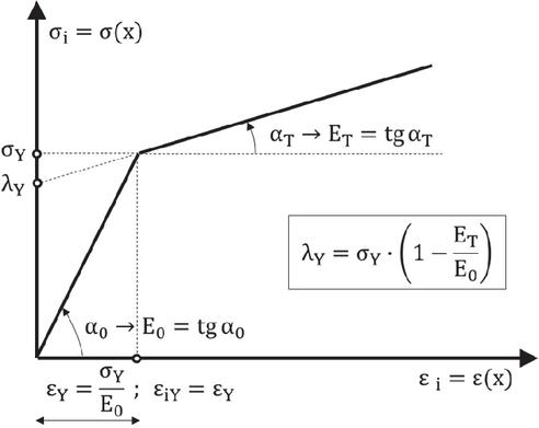
Figure 1 Bilinear $\sigma$–$\epsilon$ diagram for an elasto-plastic material with hardening.

The effective modulus $\mathrm{E}(\mathrm{x})$ for the bilinear elasto-plastic behavior of a material with initial modulus ${\mathrm{E}}_0$, yield strength ${\sigma }_{\mathrm{Y}}$, and tangential hardening modulus ${\mathrm{E}}_{\mathrm{T}}$, using the relationships from Figure 1 (${\lambda }_{\mathrm{Y}}={\sigma }_{\mathrm{Y}}\cdot (1-{\mathrm{E}}_{\mathrm{T}}/{\mathrm{E}}_0)$), has the following form [2]:

$$\mathrm{E}(\mathrm{x})=\{\begin{array}{cc}{\mathrm{E}}_0\hfill & \mathrm{for}\epsilon (\mathrm{x})\le {\epsilon }_{\mathrm{Y}}\hfill \\ {\mathrm{E}}_{\mathrm{T}}+\frac{{\lambda }_{\mathrm{Y}}}{\epsilon (\mathrm{x})}\hfill & \mathrm{for}\epsilon (\mathrm{x})>{\epsilon }_{\mathrm{Y}}\hfill \end{array}$$

(5)

Let us consider a rod of length $\mathrm{L}$ with constant cross-sectional area $\mathrm{A}$ be supported at the left end and loaded at the right end with a force $\mathrm{P}$. The rod is also loaded along its length with a continuous load $\mathrm{p}(\mathrm{x})$ as shown in Figure 2.

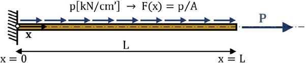
Figure 2 Geometry and loading for the 1D uniaxial example.

The analytical displacement field $\mathrm{u}(\mathrm{x})$ along the rod is obtained by solving the differential Equation (1) subject to the Dirichlet boundary condition $\mathrm{u}(0)=0$ and Neumann boundary condition $\sigma (\mathrm{L})=\mathrm{P}/\mathrm{A}=\mathrm{E}(\mathrm{L})\cdot \epsilon (\mathrm{L})={\mathrm{E}(\mathrm{L})\cdot (\mathrm{du}/\mathrm{dx})|}_{\mathrm{x}=\mathrm{L}}$:

$$u(x)=\frac{x}{A\cdot E_T}[(P-{\lambda }_Y\cdot A)-\mathrm{p}(\mathrm{x})\cdot x]$$

In the following example, we take $\mathrm{L}=100[\mathrm{cm}]$, $\mathrm{A}=4.0[{\mathrm{cm}}^2]$, $\mathrm{P}=100[\mathrm{kN}]$, ${\mathrm{E}}_0=\mathrm{10\; 000}[\mathrm{kN}/{\mathrm{cm}}^2],{\mathrm{E}}_{\mathrm{T}}=\mathrm{2\; 000}[\mathrm{kN}/{\mathrm{cm}}^2],{\sigma }_{\mathrm{Y}}=25.0[\mathrm{kN}/{\mathrm{cm}}^2]$.

For the load $\mathrm{p}(\mathrm{x})=0.1[\mathrm{kN}/\mathrm{cm}]$, the analytical displacement field has the form

$$\mathrm{u}(\mathrm{x})=\frac{\mathrm{x}\cdot (600-\mathrm{x})}{160000}$$

whereas for $\mathrm{p}(\mathrm{x})=1.0[\mathrm{kN}/\mathrm{cm}]$ it is given by

$$u(x)=\frac{x\cdot (240-x)}{16000}.$$

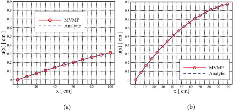
Figure 3 Comparison of the numerical solution of the displacement field with the analytical one for (a) $\mathrm{p}(\mathrm{x})=0.1\mathrm{kN}/\mathrm{cm}$ and (b) $\mathrm{p}(\mathrm{x})=1.0\mathrm{kN}/\mathrm{cm}.$

Figures 3–5 show a comparison of numerical solutions obtained by the MVMP method with known analytical solutions for a rod subjected to a continuous load $\mathrm{p}(\mathrm{x})=0.1[\mathrm{kN}/\mathrm{cm}]$ (Figures 3(a), 4(a), 5(a)), and $\mathrm{p}(\mathrm{x})=1.0[\mathrm{kN}/\mathrm{cm}]$ (Figures 3(b), 4(b), 5(b)).

The numerical solution was obtained by discretizing the area into 20 equal segments (25 basis functions Fup₄ given in Appendix A1).

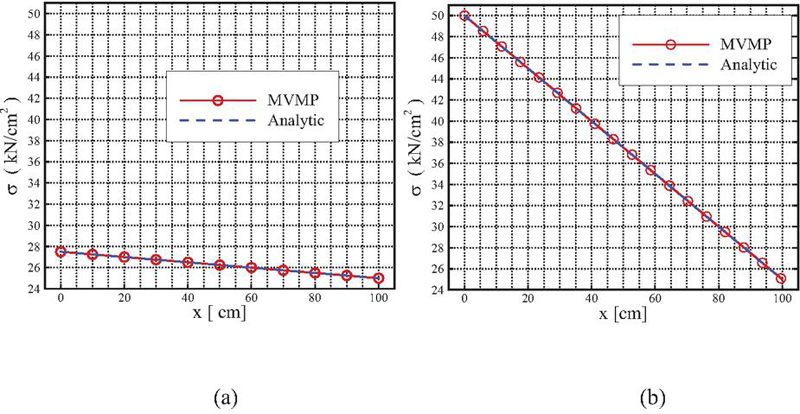
Figure 4 Comparison of the numerical solution of normal stress with the analytical one for (a) $\mathrm{p}(\mathrm{x})=0.1\mathrm{kN}/\mathrm{cm}$ and (b) $\mathrm{p}(\mathrm{x})=1.0\frac{\mathrm{kN}}{\mathrm{cm}}.$

Figures 3 and 4 show a complete overlap of the numerical solution of the displacement and stress fields with the analytical.

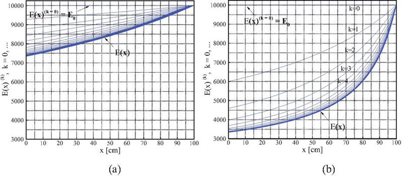
Figure 5 Changes in modulus of elasticity (Young’s modulus) along the rod by iterations (a) for $\mathrm{p}(\mathrm{x})=0.1\frac{\mathrm{kN}}{\mathrm{cm}}$ and (b) for $\mathrm{p}(\mathrm{x})=1.0\frac{\mathrm{kN}}{\mathrm{cm}}$.

Instead of a table with data on convergence, Figure 5 shows a graphic representation illustrating the change in modulus of elasticity (Young’s modulus) along the rod from the zero iteration to the final one in which the given convergence criterion is reached. Convergence of the elastic modulus field with the selected tolerance $\mathrm{tol}={10}^{-5}$ was achieved in the 20th iteration.

2.2 Theoretical Basis of the MVMP Method for Plane and Axisymmetric Problems

For bodies with variable material properties $\lambda =\lambda (\mathrm{x},\mathrm{y}),\mu =\mu (\mathrm{x},\mathrm{y})$ or $\mathrm{E}=\mathrm{E}(\mathrm{x},\mathrm{y}),\nu =\nu (\mathrm{x},\mathrm{y})$, the equilibrium equations expressed in terms of displacements, analogous to the uniaxial stress state, can be written in the following form [17]:

$${\mathrm{Q}}_{\mathrm{x}}^{\mathrm{el}}+{\mathrm{Q}}_{\mathrm{x}}^{\mathrm{pl}}+{\mathrm{F}}_{\mathrm{x}}=0$$	(6a)
$${\mathrm{Q}}_{\mathrm{x}}^{\mathrm{el}}=\frac{1}{3}\frac{{\sigma }_{\mathrm{i}}}{{\epsilon }_{\mathrm{i}}}{\nabla }^2\mathrm{u}+\left(\frac{{\mathrm{E}}_0}{3(1-2\nu )}+\frac{1}{9}\frac{{\sigma }_{\mathrm{i}}}{{\epsilon }_{\mathrm{i}}}\right)\cdot \frac{\partial \mathbf{e}}{\partial \mathrm{x}}-\mathit{\kappa }\frac{1}{3}\frac{{\sigma }_{\mathrm{i}}}{{\epsilon }_{\mathrm{i}}}\frac{\mathrm{u}}{{\mathrm{x}}^2}$$
$${\mathrm{Q}}_{\mathrm{x}}^{\mathrm{pl}}=\frac{1}{3}\frac{\partial }{\partial \mathrm{y}}\left(\frac{{\sigma }_{\mathrm{i}}}{{\epsilon }_{\mathrm{i}}}\right)\left(\frac{\partial \mathrm{u}}{\partial \mathrm{y}}+\frac{\partial \mathrm{v}}{\partial \mathrm{x}}\right)-\frac{2}{9}\frac{\partial }{\partial \mathrm{x}}\left(\frac{{\sigma }_{\mathrm{i}}}{{\epsilon }_{\mathrm{i}}}\right)\cdot \mathbf{e}+\frac{2}{3}\frac{\partial }{\partial \mathrm{x}}\left(\frac{{\sigma }_{\mathrm{i}}}{{\epsilon }_{\mathrm{i}}}\right)\cdot \frac{\partial \mathrm{u}}{\partial \mathrm{x}}$$
$${\mathrm{Q}}_{\mathrm{y}}^{\mathrm{el}}+{\mathrm{Q}}_{\mathrm{y}}^{\mathrm{pl}}+{\mathrm{F}}_{\mathrm{y}}=0$$	(6b)
$${\mathrm{Q}}_{\mathrm{y}}^{\mathrm{el}}=\frac{1}{3}\frac{{\sigma }_{\mathrm{i}}}{{\epsilon }_{\mathrm{i}}}{\nabla }^2\mathrm{v}+\left(\frac{{\mathrm{E}}_0}{3(1-2\nu )}+\frac{1}{9}\frac{{\sigma }_{\mathrm{i}}}{{\epsilon }_{\mathrm{i}}}\right)\cdot \frac{\partial \mathbf{e}}{\partial \mathrm{y}}$$
$${\mathrm{Q}}_{\mathrm{y}}^{\mathrm{pl}}=\frac{1}{3}\frac{\partial }{\partial \mathrm{x}}\left(\frac{{\sigma }_{\mathrm{i}}}{{\epsilon }_{\mathrm{i}}}\right)\left(\frac{\partial \mathrm{u}}{\partial \mathrm{y}}+\frac{\partial \mathrm{v}}{\partial \mathrm{x}}\right)-\frac{2}{9}\frac{\partial }{\partial \mathrm{y}}\left(\frac{{\sigma }_{\mathrm{i}}}{{\epsilon }_{\mathrm{i}}}\right)\cdot \mathbf{e}+\frac{2}{3}\frac{\partial }{\partial \mathrm{y}}\left(\frac{{\sigma }_{\mathrm{i}}}{{\epsilon }_{\mathrm{i}}}\right)\cdot \frac{\partial \mathrm{v}}{\partial \mathrm{y}}$$

where $\frac{{\sigma }_{\mathrm{i}}}{{\epsilon }_{\mathrm{i}}}$ is the law of behavior for both elastic and plastic area, $\mathit{\kappa }$ is a parameter that has a value equal to zero for plane problems and a value equal to one for axisymmetric problems, and ${\mathrm{F}}_{\mathrm{x}},{\mathrm{F}}_{\mathrm{y}}$ are the volume force components. ${\nabla }^2$ is the Laplace operator

$${\nabla }^2=\mathrm{△}=\frac{{\partial }^2}{\partial {\mathrm{x}}^2}+\frac{{\partial }^2}{\partial {\mathrm{y}}^2}+\frac{1}{\mathrm{x}}\cdot \frac{\partial }{\partial \mathrm{x}}$$

and $\mathbf{e}$ is the volume strain

$$\mathbf{e}=\frac{\partial \mathrm{u}}{\partial \mathrm{x}}+\frac{\partial \mathrm{v}}{\partial \mathrm{y}}+\mathit{\kappa }\frac{\mathrm{u}}{\mathrm{x}}.$$

In addition to the previous equilibrium equations, it is also necessary to specify boundary conditions:

(a) Dirichlet boundary condition: the vector displacement function at the boundary of the area is given

$$\mathrm{f}=\mathrm{f}(\mathrm{u},\mathrm{v})$$	(7a)
where $\mathrm{u},\mathrm{v}$ are the components of the displacement vector along the $\mathrm{x}$ and $\mathrm{y}$ axes, respectively.

(b) Neumann boundary condition: given a stress vector with components ${\sigma }_{\mathrm{n}}$ along the normal direction and ${\tau }_{\mathrm{n}}$ along the tangent direction at a point on the boundary of the area:

${\sigma }_{\mathrm{n}}$	$=\left({\displaystyle \frac{{\mathrm{E}}_0}{3(1-2\nu )}}+{\displaystyle \frac{4}{9}}{\displaystyle \frac{{\sigma }_{\mathrm{i}}}{{\epsilon }_{\mathrm{i}}}}\right)\cdot \left({\displaystyle \frac{\partial \mathrm{u}}{\partial \mathrm{n}}}{\mathrm{l}}_1+{\displaystyle \frac{\partial \mathrm{v}}{\partial \mathrm{n}}}{\mathrm{l}}_2\right)$
	$+\left({\displaystyle \frac{{\mathrm{E}}_0}{3(1-2\nu )}}-{\displaystyle \frac{2}{9}}{\displaystyle \frac{{\sigma }_{\mathrm{i}}}{{\epsilon }_{\mathrm{i}}}}\right)\left({\displaystyle \frac{\partial \mathrm{v}}{\partial \mathrm{t}}}{\mathrm{l}}_1-{\displaystyle \frac{\partial \mathrm{u}}{\partial \mathrm{t}}}{\mathrm{l}}_2+\mathit{\kappa }{\displaystyle \frac{\partial \mathrm{u}}{\partial \mathrm{x}}}\right)$
${\tau }_{\mathrm{n}}$	$={\displaystyle \frac{1}{3}}{\displaystyle \frac{{\sigma }_{\mathrm{i}}}{{\epsilon }_{\mathrm{i}}}}\left({\displaystyle \frac{\partial \mathrm{u}}{\partial \mathrm{n}}}{\mathrm{l}}_2-{\displaystyle \frac{\partial \mathrm{v}}{\partial \mathrm{n}}}{\mathrm{l}}_1+{\displaystyle \frac{\partial \mathrm{u}}{\partial \mathrm{t}}}{\mathrm{l}}_1+{\displaystyle \frac{\partial \mathrm{v}}{\partial \mathrm{t}}}{\mathrm{l}}_2\right)$	(7b)

The systems of Equations (6a), (6b) describe the equilibrium for the state of plane deformation and the state of axial symmetry. For the state of plane deformation, the coordinate system is Cartesian $\mathrm{x},\mathrm{y}$, and for the state of axial symmetry, the $\mathrm{x}$ axis is replaced by the $\mathrm{r}$ coordinate, the $\mathrm{y}$ axis becomes the $\mathrm{z}$ axis, and the direction of rotation has the coordinate $\varphi$. The state of plane stress can be solved by the algorithm for the state of plane deformation, with the addition of the substitute constant ${\lambda }^{\prime }=\frac{2\lambda \mu }{\lambda +2\mu }$ for the Lamé constant of the material $\lambda$.

Equations (6a), (6b) are extremely non-linear and for the numerical procedure it is necessary to carry out a suitable linearization. The volume force components ${\mathrm{F}}_{\mathrm{x}}$ and ${\mathrm{F}}_{\mathrm{y}}$, as well as all terms containing the derivative of the expression $\frac{{\sigma }_{\mathrm{i}}}{{\epsilon }_{\mathrm{i}}}$, should be placed on the right side of the equations. On the left side of the equations, there remain the terms that describe the elastic behavior for variable material properties. In this way, the task is reduced to solving a series of linear elastic problems.

3 Numerical Model for MVMP

The numerical model for solving plane and axisymmetric problems is analogous to the model for the uniaxial state of stress from Section 2.1. At the beginning of the procedure (zero iteration), the problem is solved with the default elastic properties of the material and without residual load. In the following steps (iterations), the results from the previous step are used to correct the material properties in the area of plastic deformation. The residual load and the difference in the expression for the Neumann boundary conditions must “quickly” and unconditionally tend to zero, if the basic assumptions for small elastoplastic deformations are met.

In the $(\mathrm{k}+1)$-th iteration, the elastic boundary value problem is formulated by determining two displacement functions ${\mathrm{u}}^{(\mathrm{k}+1)}(\mathrm{x},\mathrm{y})$ and ${\mathrm{v}}^{(\mathrm{k}+1)}(\mathrm{x},\mathrm{y})$ that satisfy the following differential equations in the domain $\mathrm{\Omega }$:

$${\mu }^{\ast }{\nabla }^2{\mathrm{u}}^{(\mathrm{k}+1)}+({\lambda }^{\ast }+{\mu }^{\ast })\frac{\partial {\mathbf{e}}^{(\mathrm{k}+1)}}{\partial \mathrm{x}}-\mathit{\kappa }\cdot {\mu }^{\ast }\frac{{\mathrm{u}}^{(\mathrm{k}+1)}}{{\mathrm{x}}^2}=-({\mathrm{F}}_{\mathrm{x}}+\mathrm{F}_{\mathrm{x}}^{}{}_{}{}^{(\mathrm{k}+1)})$$	(8a)
$${\mu }^{\ast }{\nabla }^2{\mathrm{v}}^{(\mathrm{k}+1)}+({\lambda }^{\ast }+{\mu }^{\ast })\frac{\partial {\mathbf{e}}^{(\mathrm{k}+1)}}{\partial \mathrm{y}}=-({\mathrm{F}}_{\mathrm{y}}+\mathrm{F}_{\mathrm{y}}^{}{}_{}{}^{(\mathrm{k}+1)})$$	(8b)

and on the boundary $\mathrm{\Gamma }$ for Neumann boundary conditions

$({\lambda }^{\ast }+2{\mu }^{\ast })\left({\displaystyle \frac{\partial {\mathrm{u}}^{(\mathrm{k}+1)}}{\partial \mathrm{n}}}{\mathrm{l}}_1+{\displaystyle \frac{\partial {\mathrm{v}}^{(\mathrm{k}+1)}}{\partial \mathrm{n}}}{\mathrm{l}}_2\right)$
$+{\lambda }^{\ast }\left({\displaystyle \frac{\partial {\mathrm{v}}^{(\mathrm{k}+1)}}{\partial \mathrm{t}}}{\mathrm{l}}_1-{\displaystyle \frac{\partial {\mathrm{u}}^{(\mathrm{k}+1)}}{\partial \mathrm{t}}}{\mathrm{l}}_2+\mathit{\kappa }\cdot {\mu }^{\ast }{\displaystyle \frac{\partial {\mathrm{u}}^{(\mathrm{k})}}{\partial \mathrm{x}}}\right)={\mathrm{f}}_{\mathrm{n}}-\mathrm{f}_{\mathrm{n}}^{}{}_{}{}^{(\mathrm{k}+1)}$	(9a)
${\mu }^{\ast }\left({\displaystyle \frac{\partial {\mathrm{u}}^{(\mathrm{k}+1)}}{\partial \mathrm{n}}}{\mathrm{l}}_2-{\displaystyle \frac{\partial {\mathrm{v}}^{(\mathrm{k}+1)}}{\partial \mathrm{n}}}{\mathrm{l}}_1+{\displaystyle \frac{\partial {\mathrm{u}}^{(\mathrm{k}+1)}}{\partial \mathrm{t}}}{\mathrm{l}}_1+{\displaystyle \frac{\partial {\mathrm{v}}^{(\mathrm{k}+1)}}{\partial \mathrm{t}}}{\mathrm{l}}_2\right)={\mathrm{f}}_{\mathrm{t}}-\mathrm{f}_{\mathrm{t}}^{}{}_{}{}^{(\mathrm{k}+1)}$	(9b)

where ${\lambda }^{\ast }$ and ${\mu }^{\ast }$ are Lamé’s elastic parameters in the $\mathrm{k}$-th step or iteration.

Volume deformation $\mathbf{e}$ becomes

$${\mathbf{e}}^{(\mathrm{k}+1)}=\frac{\partial {\mathrm{u}}^{(\mathrm{k}+1)}}{\partial \mathrm{x}}+\frac{\partial {\mathrm{v}}^{(\mathrm{k}+1)}}{\partial \mathrm{y}}+\mathit{\kappa }\frac{{\mathrm{u}}^{(\mathrm{k}+1)}}{\mathrm{x}}.$$

In Equations (9a), (9b), ${\mathrm{f}}_{\mathrm{n}}$ and ${\mathrm{f}}_{\mathrm{t}}$ denote the projections of the surface load vector along the normal and tangent lines at the edge point of the area, respectively.

In the area of plastic deformation, material properties change, which leads to residual volume forces $\mathrm{F}_{\mathrm{x}}^{}{}_{}{}^{(\mathrm{k}+1)}$ and $\mathrm{F}_{\mathrm{y}}^{}{}_{}{}^{(\mathrm{k}+1)}$, and surface forces $\mathrm{f}_{\mathrm{n}}^{}{}_{}{}^{(\mathrm{k}+1)}$ and $\mathrm{f}_{\mathrm{t}}^{}{}_{}{}^{(\mathrm{k}+1)}$ in the following form:

$\mathrm{F}_{\mathrm{x}}^{}{}_{}{}^{(\mathrm{k}+1)}$	$={\displaystyle \frac{\partial }{\partial \mathrm{x}}}\left[\left(2\mu -{\displaystyle \frac{2}{3}}{\displaystyle \frac{\sigma _{\mathrm{i}}^{}{}_{}{}^{(\mathrm{k})}}{\epsilon _{\mathrm{i}}^{}{}_{}{}^{(\mathrm{k})}}}\right)\cdot \left({\displaystyle \frac{2}{3}}{\displaystyle \frac{\partial {\mathrm{u}}^{(\mathrm{k})}}{\partial \mathrm{x}}}-{\displaystyle \frac{1}{3}}{\displaystyle \frac{\partial {\mathrm{v}}^{(\mathrm{k})}}{\partial \mathrm{y}}}\right)\right]$
	$+{\displaystyle \frac{\partial }{\partial \mathrm{y}}}\left[\left(\mu -{\displaystyle \frac{1}{3}}{\displaystyle \frac{\sigma _{\mathrm{i}}^{}{}_{}{}^{(\mathrm{k})}}{\epsilon _{\mathrm{i}}^{}{}_{}{}^{(\mathrm{k})}}}\right)\cdot \left({\displaystyle \frac{\partial {\mathrm{u}}^{(\mathrm{k})}}{\partial \mathrm{y}}}+{\displaystyle \frac{\partial {\mathrm{v}}^{(\mathrm{k})}}{\partial \mathrm{x}}}\right)\right]$
$\mathrm{F}_{\mathrm{y}}^{}{}_{}{}^{(\mathrm{k}+1)}$	$={\displaystyle \frac{\partial }{\partial \mathrm{x}}}\left[\left(\mu -{\displaystyle \frac{1}{3}}{\displaystyle \frac{\sigma _{\mathrm{i}}^{}{}_{}{}^{(\mathrm{k})}}{\epsilon _{\mathrm{i}}^{}{}_{}{}^{(\mathrm{k})}}}\right)\cdot \left({\displaystyle \frac{\partial {\mathrm{u}}^{(\mathrm{k})}}{\partial \mathrm{y}}}+{\displaystyle \frac{\partial {\mathrm{v}}^{(\mathrm{k})}}{\partial \mathrm{x}}}\right)\right]$
	$+{\displaystyle \frac{\partial }{\partial \mathrm{y}}}\left[\left(2\mu -{\displaystyle \frac{2}{3}}{\displaystyle \frac{\sigma _{\mathrm{i}}^{}{}_{}{}^{(\mathrm{k})}}{\epsilon _{\mathrm{i}}^{}{}_{}{}^{(\mathrm{k})}}}\right)\cdot \left({\displaystyle \frac{2}{3}}{\displaystyle \frac{\partial {\mathrm{u}}^{(\mathrm{k})}}{\partial \mathrm{x}}}-{\displaystyle \frac{1}{3}}{\displaystyle \frac{\partial {\mathrm{v}}^{(\mathrm{k})}}{\partial \mathrm{y}}}\right)\right]$	(10)
$\mathrm{f}_{\mathrm{n}}^{}{}_{}{}^{(\mathrm{k}+1)}$	$=\left(2\mu -{\displaystyle \frac{2}{3}}{\displaystyle \frac{\sigma _{\mathrm{i}}^{}{}_{}{}^{(\mathrm{k})}}{\epsilon _{\mathrm{i}}^{}{}_{}{}^{(\mathrm{k})}}}\right)\cdot \left({\displaystyle \frac{\partial {\mathrm{u}}^{(\mathrm{k})}}{\partial \mathrm{y}}}+{\displaystyle \frac{\partial {\mathrm{v}}^{(\mathrm{k})}}{\partial \mathrm{x}}}\right){\mathrm{l}}_1{\mathrm{l}}_2$
	$+\left(2\mu -{\displaystyle \frac{2}{3}}{\displaystyle \frac{\sigma _{\mathrm{i}}^{}{}_{}{}^{(\mathrm{k})}}{\epsilon _{\mathrm{i}}^{}{}_{}{}^{(\mathrm{k})}}}\right)\cdot \left({\displaystyle \frac{2}{3}}{\displaystyle \frac{\partial {\mathrm{u}}^{(\mathrm{k})}}{\partial \mathrm{x}}}-{\displaystyle \frac{1}{3}}{\displaystyle \frac{\partial {\mathrm{v}}^{(\mathrm{k})}}{\partial \mathrm{y}}}\right){\mathrm{l}}_1^2$
	$+\left(2\mu -{\displaystyle \frac{2}{3}}{\displaystyle \frac{\sigma _{\mathrm{i}}^{}{}_{}{}^{(\mathrm{k})}}{\epsilon _{\mathrm{i}}^{}{}_{}{}^{(\mathrm{k})}}}\right)\cdot \left({\displaystyle \frac{2}{3}}{\displaystyle \frac{\partial {\mathrm{v}}^{(\mathrm{k})}}{\partial \mathrm{y}}}-{\displaystyle \frac{1}{3}}{\displaystyle \frac{\partial {\mathrm{u}}^{(\mathrm{k})}}{\partial \mathrm{x}}}\right){\mathrm{l}}_2^2$
$\mathrm{f}_{\mathrm{t}}^{}{}_{}{}^{(\mathrm{k}+1)}$	$=\left(\mu -{\displaystyle \frac{1}{3}}{\displaystyle \frac{\sigma _{\mathrm{i}}^{}{}_{}{}^{(\mathrm{k})}}{\epsilon _{\mathrm{i}}^{}{}_{}{}^{(\mathrm{k})}}}\right)\cdot \left({\displaystyle \frac{\partial {\mathrm{u}}^{(\mathrm{k})}}{\partial \mathrm{y}}}+{\displaystyle \frac{\partial {\mathrm{v}}^{(\mathrm{k})}}{\partial \mathrm{x}}}\right)\left({\mathrm{l}}_2^2-{\mathrm{l}}_1^2\right)$
	$+\left(2\mu -{\displaystyle \frac{2}{3}}{\displaystyle \frac{\sigma _{\mathrm{i}}^{}{}_{}{}^{(\mathrm{k})}}{\epsilon _{\mathrm{i}}^{}{}_{}{}^{(\mathrm{k})}}}\right)\cdot \left({\displaystyle \frac{\partial {\mathrm{u}}^{(\mathrm{k})}}{\partial \mathrm{x}}}-{\displaystyle \frac{\partial {\mathrm{v}}^{(\mathrm{k})}}{\partial \mathrm{y}}}\right){\mathrm{l}}_1{\mathrm{l}}_2$	(11)

In Equations (10) and (11), $\mu$ denotes the initial parameter of the material.

According to the method of variable material properties (MVMP), the elastic modulus ${\mathrm{E}}^{\ast }$ and Poisson’s ratio ${\nu }^{\ast }$ depend on the relationship between stress and strain in the material, and are calculated using [17]:

$${\mathrm{E}}^{\ast }=\frac{\frac{{\sigma }_{\mathrm{i}}}{{\epsilon }_{\mathrm{i}}}}{1+\frac{(1-2\nu )}{3{\mathrm{E}}_0}\cdot \frac{{\sigma }_{\mathrm{i}}}{{\epsilon }_{\mathrm{i}}}};{\nu }^{\ast }=\frac{\frac{1}{2}-\frac{(1-2\nu )}{3{\mathrm{E}}_0}\frac{{\sigma }_{\mathrm{i}}}{{\epsilon }_{\mathrm{i}}}}{1+\frac{(1-2\nu )}{3{\mathrm{E}}_0}\frac{{\sigma }_{\mathrm{i}}}{{\epsilon }_{\mathrm{i}}}}.$$

(12)

The Lamé parameters ${\lambda }^{\ast }$ and ${\mu }^{\ast }$ are also functions of the coordinates and are determined based on the solution of the problem at the end of the previous iteration:

${\lambda }^{\ast }$	$={\displaystyle \frac{{\mathrm{E}}^{\ast }{\nu }^{\ast }}{(1-2{\nu }^{\ast })(1+{\nu }^{\ast })}}\to {\lambda }^{(\mathrm{k}+1)}={\displaystyle \frac{{\mathrm{E}}_0}{3(1-2\nu )}}-{\displaystyle \frac{2}{9}}\cdot {\displaystyle \frac{\sigma _{\mathrm{i}}^{}{}_{}{}^{(\mathrm{k})}}{\epsilon _{\mathrm{i}}^{}{}_{}{}^{(\mathrm{k})}}}$
${\mu }^{\ast }$	$={\displaystyle \frac{{\mathrm{E}}^{\ast }}{2(1+{\nu }^{\ast })}}\to {\mu }^{(\mathrm{k}+1)}={\displaystyle \frac{1}{3}}{\displaystyle \frac{\sigma _{\mathrm{i}}^{}{}_{}{}^{(\mathrm{k})}}{\epsilon _{\mathrm{i}}^{}{}_{}{}^{(\mathrm{k})}}}$	(13)

${\epsilon }_{\mathrm{i}}$ is the equivalent strain used to test whether the material at a point in the region has exceeded the limit of linear elastic behavior. If so, the equivalent stress ${\sigma }_{\mathrm{i}}$ is calculated according to the behavior law diagram, and then the values of the Lamé parameters ${\lambda }^{\ast }$ and ${\mu }^{\ast }$ in the (k+1)th iteration are determined according to Equation (13). The equivalent strain ${\epsilon }_{\mathrm{i}}$ is calculated by:

$\epsilon _{\mathrm{i}}^{}{}_{}{}^{(\mathrm{k})}$	$={\displaystyle \frac{\sqrt{2}}{3}}\cdot [{({\displaystyle \frac{\partial {\mathrm{u}}^{(\mathrm{k})}}{\partial \mathrm{x}}}-{\displaystyle \frac{\partial {\mathrm{v}}^{(\mathrm{k})}}{\partial \mathrm{y}}})}^2+{({\displaystyle \frac{\partial {\mathrm{u}}^{(\mathrm{k})}}{\partial \mathrm{x}}}-\kappa {\displaystyle \frac{\partial {\mathrm{u}}^{(\mathrm{k})}}{\partial \mathrm{x}}})}^2$
	$+{({\displaystyle \frac{\partial {\mathrm{v}}^{(\mathrm{k})}}{\partial \mathrm{y}}}-\kappa {\displaystyle \frac{{\mathrm{u}}^{(\mathrm{k})}}{\mathrm{x}}})}^2+{\displaystyle \frac{3}{2}}{({\displaystyle \frac{\partial {\mathrm{u}}^{(\mathrm{k})}}{\partial \mathrm{y}}}+{\displaystyle \frac{\partial {\mathrm{v}}^{(\mathrm{k})}}{\partial \mathrm{x}}})}^2]{}^{1/2}$	(14)

As already mentioned, at the beginning of the numerical process the parameters ${\mathrm{E}}^{\ast }={\mathrm{E}}_0$, ${\nu }^{\ast }=\nu$ are used and in the initial iteration the problem of an elastic isotropic body is solved, where

$$\frac{{\sigma }_{\mathrm{i}}}{{\epsilon }_{\mathrm{i}}}=\frac{3{\mathrm{E}}_0}{2(1+\nu )}.$$

(15)

4 MVMP Algorithm

The proposed numerical implementation algorithm of MVMP using ABF Fup₄ and the collocation method consists of the steps described below.

4.1 Initialization

Setting the geometry, boundary conditions, elastic material parameters (${\mathrm{E}}_0,{\nu }_0$) and Lamé’s constants (${\lambda }_0,{\mu }_0$); discretization of the domain with equal segments $\mathrm{\Delta }\mathrm{x}$ in 1D problems (rod), $\mathrm{\Delta }$x and $\mathrm{\Delta }$y for the plane states, or $\mathrm{\Delta }$r and $\mathrm{\Delta }$z for axisymmetric problems; constructing the base of Fup₄ functions.

4.2 Initial Assumption

The material is treated as elastic with known initial values ${\mathrm{E}}_0$ and ${\nu }_0$, or Lamé coefficients ${\lambda }_0$ and ${\mu }_0$.

4.3 Stress and Strain Calculations

From the obtained displacements ${\mathrm{u}}^{(\mathrm{k})}$, the deformation and stress components are determined, from which the equivalent deformation $\epsilon _{\mathrm{i}}^{}{}_{}{}^{(\mathrm{k})}$ is calculated according to Equation (3) and the corresponding equivalent stress $\sigma _{\mathrm{i}}^{}{}_{}{}^{(\mathrm{k})}$ is calculated from the material behavior diagram.

4.4 Updating Material Parameters

For each collocation point, the value $\epsilon _{\mathrm{i}}^{}{}_{}{}^{(\mathrm{k})}$ is tested. If $\epsilon _{\mathrm{i}}^{}{}_{}{}^{(\mathrm{k})}\le {\epsilon }_{\mathrm{Y}}$, the linear elastic parameters are retained, and if $\epsilon _{\mathrm{i}}^{}{}_{}{}^{(\mathrm{k})}>{\epsilon }_{\mathrm{Y}}$, the hardening law is applied according to Equation (12). From ${\mathrm{E}}^{\ast }$ and ${\nu }^{\ast }$, ${\lambda }^{\ast }$ and ${\mu }^{\ast }$ are calculated according to (13).

4.5 Calculating the Values of the Material Properties

Since the derivatives of the material parameters are needed in the plastic area, they are approximated by Fup₄ basis functions. The coefficients of the basis functions ${\mathrm{C}}_{\mathrm{j}}$ are obtained by an iterative process so that the solution in the kth step represents the start vector for the (k+1) iterative step.

4.6 Solving the System

The system of Equations (8)–(11) is solved.

4.7 Convergence Criterion

The displacement norm ${\Vert \mathrm{u}(\mathrm{k}+1)-\mathrm{u}(\mathrm{k})\Vert }^2$ is calculated. If $\parallel \cdot {\parallel }^2\le \mathrm{tol}$, the procedure is stopped; otherwise, the iteration procedure continues until the convergence criterion is met.

4.8 Output Results

The displacement fields are calculated and the stress and strain fields are derived. The fields of changes in the material parameters $\mathrm{E}(\mathrm{x}),\nu (\mathrm{x}),\lambda (\mathrm{x}),\mu (\mathrm{x})$ are also determined, which illustrate the plasticized zone.

5 Example: Thin Disc Loaded with Internal Pressure

A thin disc with a circular hole around the center is considered, which is in an elastoplastic state of deformation (Figure 6). The material from which the disc is made is incompressible without hardening (${\sigma }_{\mathrm{i}}=\mathrm{const}.={\sigma }_{\mathrm{Y}},{\epsilon }_0=0,\nu =1/2$). With these assumptions, it is possible to obtain a closed-form solution. This allows a comparison of the analytical and numerical solutions.

If $\mathrm{t}\ll {\mathrm{r}}_2$, the problem is consistent with the assumptions for a plane stress state. Also, the problem is consistent with the assumptions for a axial symmetry state.

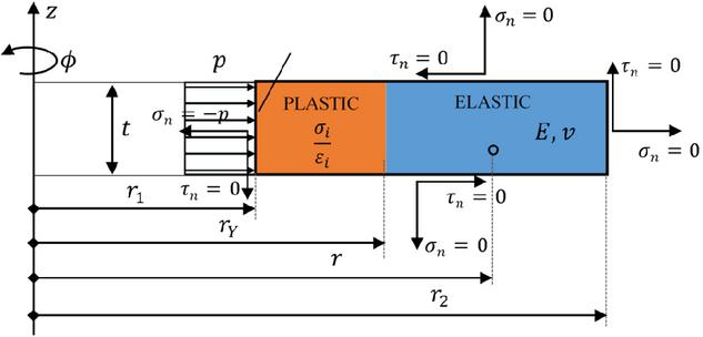
Figure 6 Geometry of a disc with a circular hole around the center.

The load acting on the disc is the pressure on the inner edge, while the other surfaces are unloaded. The input parameters are:

${\mathrm{r}}_1=4[\mathrm{cm}]$ inner radius

${\mathrm{r}}_2=10[\mathrm{cm}]$ outer radius

${\mathrm{E}}_0=\mathrm{10\; 000}[\mathrm{kN}/{\mathrm{cm}}^2]$ Young’s modulus

$\nu =0.5(0.49999)$ Poisson’s ratio, the value in brackets is used in the numerical procedure

${\sigma }_{\mathrm{Y}}=25[\mathrm{kN}/{\mathrm{cm}}^2]$ yield stress

${\mathrm{E}}_{\mathrm{T}}=0$ tangent modulus of hardening

$\mathrm{p}=20[\mathrm{kN}/{\mathrm{cm}}^2]$ pressure on the inner surface

$\mathrm{t}=1[\mathrm{cm}]$ disc thickness

${\mathrm{r}}_{\mathrm{Y}}=5.786105[\mathrm{cm}]$ radius of the boundary between the elastic and plastic parts

${\mathrm{\Psi }}_1=\mathrm{\Psi }({\mathrm{r}}_1)=2.336189$ value on the inner edge

${\mathrm{\Psi }}_{\mathrm{Y}}=\mathrm{\Psi }({\mathrm{r}}_{\mathrm{Y}})=1.903459$ value at the boundary of the elastic and plastic deformation range

The symbols ${\mathrm{r}}_{\mathrm{Y}}$, ${\mathrm{\Psi }}_1$ and ${\mathrm{\Psi }}_{\mathrm{Y}}$ are used in the analytical procedure (see Appendix A2).

The selected example fulfills the basic conditions of the plane stress state and it is possible to obtain a closed-form solution given in Appendix A2. The selected example also fulfills all the conditions for the axial symmetry state. The numerical procedure described in the algorithm in Section 4 was used for the solution.

Figure 7 shows a comparison of the obtained numerical solution of the displacement and stress fields with the analytical solutions. It can be observed that the values of displacement and stresses obtained by the method proposed in this paper perfectly match the exact solution in both the elastic and plastic parts of the area.

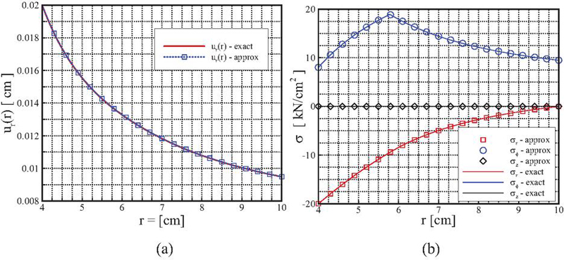
Figure 7 (a) Displacements ${\mathrm{u}}_{\mathrm{r}}(\mathrm{r})$ and (b) stresses ${\sigma }_{\mathrm{r}}(\mathrm{r}),{\sigma }_{\varphi }(\mathrm{r}),{\sigma }_{\mathrm{z}}(\mathrm{r})$.

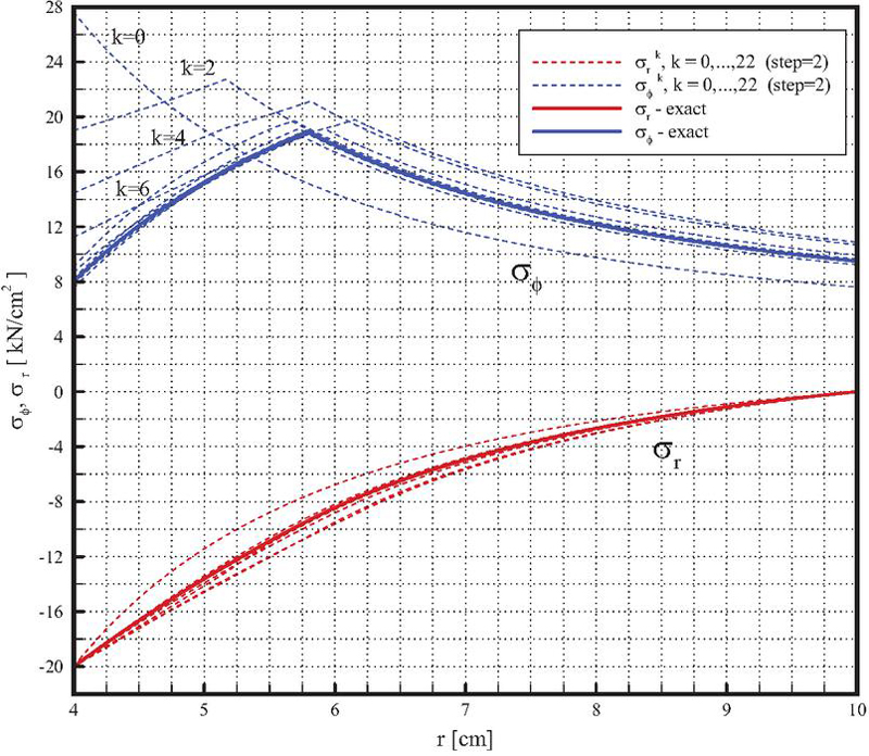
Figure 8 Illustration of the convergence process through stress calculations ${\sigma }_{\varphi }(\mathrm{r})$ and ${\sigma }_{\mathrm{r}}(\mathrm{r})$.

Figure 8 shows a graphic representation that illustrates the process of convergence through the calculation of stresses ${\sigma }_{\varphi }(\mathrm{r})$ and ${\sigma }_{\mathrm{r}}(\mathrm{r})$. From Figure 8, it is possible to see the regularity of changing the parameters of the material by which the stress components are calculated according to iterative steps. A total of 40 iterations were used to obtain the numerical solution. It is evident that already in the first 10 iterations, the numerical solution approached the analytical values. For the point on the inner edge of the disc (r $=$ r₁), Figure 9 shows the changes in the elastic properties of the material, from the zero iterative step where the initial parameters are E₀ and ${\nu }_0$, to the last iteration. From Figure 9, it is evident that the numerical solution for the material parameters practically coincides with the analytical one after about 30 iteration steps.

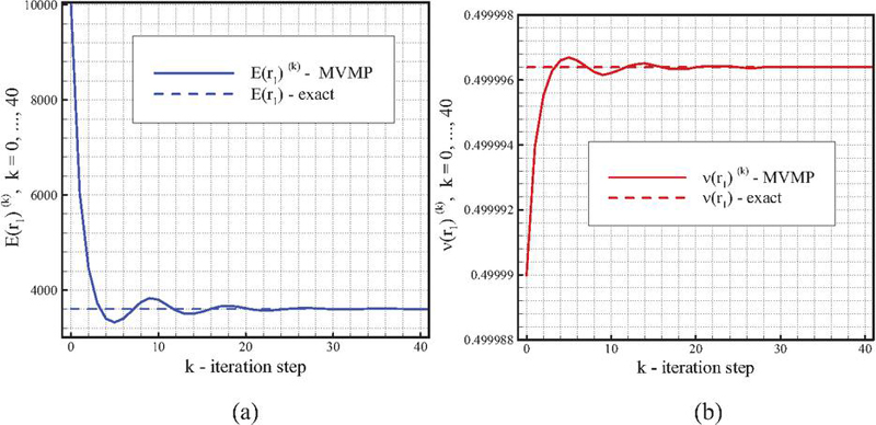
Figure 9 Convergence of material parameter values at the point $\mathrm{r}=4[\mathrm{cm}]$ (a) elastic modulus ${\mathrm{E}}^{\ast }$ and (b) Poisson’s ratio ${\nu }^{\ast }$.

6 Conclusion

The proposed MVMP-ABF procedure solves elastoplastic problems as a series of linear elastic tasks, where the nonlinearity is mapped into residual volume and boundary terms, and also into spatially variable elastic parameters ($\lambda ,\mu$) that are iteratively updated. This avoids the classical formation and updating of tangent stiffness, and the focus shifts to stable collocational discretization and smooth reconstruction of the material property field.

A key step of the method is the linearization of the differential equation where all terms involving gradients of material parameters ($\nabla \lambda$, $\nabla \mu$) and induced volume/surface forces are moved to the right-side of the equation, while the left-side remains an elastic operator with currently ‘frozen’ properties. This provides a clear demarcation between the ‘main’ linear problem and the ‘residual’ correction. The algorithm of successive approximations is carried out until the stopping criterion is met. With the assumptions of small elastoplastic deformations, the residual terms quickly tend to zero.

The collocation method with the application of ABF Fup₄ basis functions ensures that the higher derivatives required in the strong form are calculated stably, without oscillations and without the need for remeshing. Compared to the FEM-variants MVMP/VEP, which often update only the modulus of elasticity E per element, here the Lamé constants $\lambda$ and $\mu$ are simultaneously updated as smooth fields, which reduces discontinuities in stresses and enables C¹ continuity, especially in the transition zone from the elastic to the plastic region.

The method was verified on two classic examples that have analytical solutions. Numerical solutions obtained by the proposed method for an axially loaded 1D rod and an axisymmetric disc under the action of internal pressure show a fast convergence and, at the end of the iterative process, an excellent match with the analytical solutions of the mentioned problems.

Acknowledgments

This research is partially supported through project KK.01.1.1.02.0027, a project co-financed by the Croatian Government and the European Union through the European Regional Development Fund – Competitiveness and Cohesion Operational Programme.

Appendix

A1 Atomic Basis Functions

The simplest and basic atomic function is up(x). The up(x) function does not have an analytical record but is generated using a special order that is numerically calculated. It is possible to calculate the function up(x) and its derivatives up to machine precision, but this approach is sufficient for all practical purposes. Mathematical expressions for Fup_n(x) and their derivatives are obtained using linear combinations of shifted up(x) functions and their derivatives, respectively. All details regarding the calculation of the function up(x) values and values of Fup_n(x) and their derivatives are provided in [13–15].

${\mathrm{Fup}}_{\mathrm{n}}$ are finite ${\mathrm{C}}^{\mathrm{\infty }}$ functions with compact support that accurately describe polynomials up to degree $\mathrm{n}$. For $\mathrm{n}=4$ (${\mathrm{Fup}}_4)$, high smoothness is obtained with a small support, which is favorable for strong formulations where multiple derivatives appear. Figure A1 shows the basis function Fup₄ and its first four derivatives.

The support of the function contains six characteristic segments. By linearly combining these functions shifted by the length of the characteristic segment, algebraic polynomials up to degree 4 can be accurately represented. The basis on the interval is built by shifting the function Fup₄ by the characteristic segment.

In order for the collocation method on the domain to be effectively implemented using these basis functions, it is necessary to write additional conditional equations for the basis functions that have nonzero values inside the domain and whose vertices are outside the domain. These equations are based on the condition that the fifth derivative on two segments along the boundary of the domain is equal to zero. Compared to splines, the Fup₄ basis requires fewer functions for the same level of accuracy and provides smoother derivative diagrams.

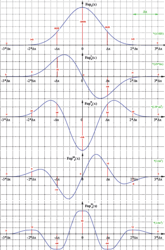
Figure A1: Function Fup₄ and its first four derivatives.

A2 Analytical Solution of a Thin Disc Loaded with Internal Pressure

A closed-form solution was obtained [2] with the assumptions that ${\mathrm{E}}_{\mathrm{T}}=0$, and that the material is incompressible, ${\epsilon }_0=0$. Poisson’s coefficient is $\nu =0.5$ or $\nu =0.49999$ for the numerical procedure. In this case, for the plane state of stress in the plastic area of deformation, the stress components are:

$${\sigma }_{\mathrm{r}}^{\mathrm{pl}}=\frac{2}{\sqrt{3}}{\sigma }_{\mathrm{Y}}\cos (\mathrm{\Psi }(\mathrm{r}));{\sigma }_{\varphi }^{\mathrm{pl}}=\frac{2}{\sqrt{3}}{\sigma }_{\mathrm{Y}}\cos \left({\mathrm{\Psi }}_{\mathrm{r}}-\frac{\pi }{3}\right).$$

(A1)

The Huber-Misses plasticity condition (${\sigma }_{\mathrm{r}}^2+{\sigma }_{\varphi }^2-{\sigma }_{\mathrm{r}}{\sigma }_{\varphi }=\sigma _{\mathrm{Y}}^{}{}_{}{}^2)$ is unconditionally fulfilled in the area of plastic deformation.

The function $\mathrm{\Psi }(\mathrm{r})$ for the selected radius $\mathrm{r}$ is determined numerically from the following equation:

$$\frac{\mathrm{r}}{{\mathrm{r}}_1}={\left[{\mathrm{e}}^{\sqrt{3}({\mathrm{\Psi }}_1-\mathrm{\Psi }(\mathrm{r}))}\cdot \frac{\sin \left({\mathrm{\Psi }}_1-\frac{\pi }{6}\right)}{\sin (\mathrm{\Psi }(\mathrm{r})-\frac{\pi }{6})}\right]}^{1/2}$$

where, from the Neumann boundary condition $\sigma ({\mathrm{r}}_1)=-\mathrm{p}$, it follows

$${\mathrm{\Psi }}_1=\arccos \left(-\frac{\sqrt{3}}{2}\frac{\mathrm{p}}{{\sigma }_{\mathrm{Y}}}\right);{\mathrm{\Psi }}_1=\mathrm{\Psi }({\mathrm{r}}_1);{\mathrm{\Psi }}_{\mathrm{Y}}=\mathrm{\Psi }({\mathrm{r}}_{\mathrm{Y}}).$$

(A2)

The function ${\mathrm{\Psi }}_{\mathrm{Y}}$ at the boundary between the elastic and plastic regions is determined by numerically solving the following transcendental equation:

$$\frac{{\mathrm{r}}_2}{{\mathrm{r}}_1}={\left[\frac{1}{\sqrt{3}}{\mathrm{e}}^{\sqrt{3}({\mathrm{\Psi }}_1-{\mathrm{\Psi }}_{\mathrm{Y}})}\cdot \frac{\sin ({\mathrm{\Psi }}_1-\frac{\pi }{6})}{\cos ({\mathrm{\Psi }}_{\mathrm{Y}}-\frac{\pi }{6})}\right]}^{1/2}$$

(A3)

and the radius ${\mathrm{r}}_{\mathrm{Y}}$ between the elastic and plastic regions

$$\frac{{\mathrm{r}}_{\mathrm{Y}}}{{\mathrm{r}}_2}=\frac{\sqrt[4]{3}}{\sqrt{\mathrm{tg}({\mathrm{\Psi }}_{\mathrm{Y}}-\frac{\pi }{6})}}.$$

(A4)

The stress components in the elastic region of deformation are determined from the remaining three conditions:

$${\sigma }_{\mathrm{r}}^{\mathrm{el}}({\mathrm{r}}_2)=0,{\sigma }_{\mathrm{r}}^{\mathrm{el}}({\mathrm{r}}_{\mathrm{Y}})={\sigma }_{\mathrm{r}}^{\mathrm{pl}}({\mathrm{r}}_{\mathrm{Y}}),{\sigma }_{\varphi }^{\mathrm{el}}({\mathrm{r}}_{\mathrm{Y}})={\sigma }_{\varphi }^{\mathrm{pl}}({\mathrm{r}}_{\mathrm{Y}}),$$

$${\sigma }_{\mathrm{r}}^{\mathrm{pl}}={\sigma }_{\mathrm{Y}}\cos \left({\mathrm{\Psi }}_{\mathrm{Y}}-\frac{\pi }{6}\right)\left(1-{\left(\frac{{\mathrm{r}}_2}{\mathrm{r}}\right)}^2\right);$$

$${\sigma }_{\varphi }^{\mathrm{pl}}={\sigma }_{\mathrm{Y}}\cos \left({\mathrm{\Psi }}_{\mathrm{Y}}-\frac{\pi }{6}\right)\left(1+{\left(\frac{{\mathrm{r}}_2}{\mathrm{r}}\right)}^2\right)$$

Radial displacements in the plastic and elastic regions are calculated using:

$${\mathrm{u}}_{\mathrm{pl}}(\mathrm{r})=\frac{{\sigma }_{\mathrm{r}}\cdot {\mathrm{r}}_{\mathrm{Y}}}{\mathrm{E}}\sin ({\mathrm{\Psi }}_{\mathrm{Y}})\cdot {\mathrm{e}}^{\sqrt{\frac{3}{2}(\mathrm{\Psi }-{\mathrm{\Psi }}_{\mathrm{Y}})}}\cdot {\left[\frac{\sin ({\mathrm{\Psi }}_{\mathrm{Y}}-\frac{\pi }{6})}{\sin (\mathrm{\Psi }-\frac{\pi }{6})}\right]}^{\frac{1}{2}}$$

$${\mathrm{u}}_{\mathrm{el}}(\mathrm{r})=\frac{{\sigma }_{\mathrm{Y}}\cdot \mathrm{r}}{2\mathrm{E}}\cos \left({\mathrm{\Psi }}_{\mathrm{Y}}-\frac{\pi }{6}\right)\cdot \left(1+3{\left(\frac{{\mathrm{r}}_2}{\mathrm{r}}\right)}^2\right)$$

The critical load ${\mathrm{p}}_{\mathrm{cr}}({\mathrm{r}}_1)$ that leads to the beginning of the plasticization front is determined by the plasticity condition ${\sigma }_{\mathrm{r}}^2+{\sigma }_{\varphi }^2-{\sigma }_{\mathrm{r}}{\sigma }_{\varphi }={\sigma }_{\mathrm{Y}}^2$.

Including stress components ${\sigma }_{\mathrm{r}}$ and ${\sigma }_{\varphi }$ according to Equation (A1), the critical load is obtained:

$${\mathrm{p}}_{\mathrm{cr}}={\sigma }_{\mathrm{T}}\frac{{\mathrm{r}}_2^2-\mathrm{r}_1^{}{}_{}{}^2}{\sqrt{{\mathrm{r}}_1^4+3{\mathrm{r}}_2^4}}.$$

By increasing the load, the area of plastic deformation expands. At ${\mathrm{r}}_{\mathrm{Y}}={\mathrm{r}}_2$, the bearing capacity of the section from ${\mathrm{r}}_1$ to ${\mathrm{r}}_2$ is exhausted. From (A4) it follows that ${\mathrm{\Psi }}_{\mathrm{Y}}=\pi /2$, where the Equation (A3) becomes

$${\left(\frac{{\mathrm{r}}_2}{{\mathrm{r}}_1}\right)}^2=\frac{2}{\sqrt{3}}{\mathrm{e}}^{\sqrt{3}({\mathrm{\Psi }}_1-\pi /2)}\cdot \sin \left({\mathrm{\Psi }}_1-\frac{\pi }{6}\right).$$

(A5)

${\mathrm{\Psi }}_1$ can be determined from the known relationship ${\mathrm{r}}_2/{\mathrm{r}}_1$, and after that the corresponding load is determined from (A1).

From Equation (A1) it can be concluded that the highest load occurs at ${\mathrm{\Psi }}_1=\pi$ and it amounts to

$${\mathrm{p}}_{\max }=\frac{2}{\sqrt{3}}{\sigma }_{\mathrm{Y}}.$$

The size ${\mathrm{\Psi }}_1=\pi$ in accordance with Equation (A5) gives ${\mathrm{r}}_2/{\mathrm{r}}_1=2.963$. If the ratio ${\mathrm{r}}_2/{\mathrm{r}}_1$ is greater than 2.963 then, for any load up to ${\mathrm{p}}_{\max }$, part of the section from ${\mathrm{r}}_1$ to ${\mathrm{r}}_2$ remains in the elastic area of deformation.

References

[1] J H Snoeijer, A Pandey, M A Herrada and J Eggers. (2020). The relationship between viscoelasticity and elasticity. Proc R Soc A, 476(2243):2020049.

[2] I A Birger. (1963). Residual stresses. Moscow: Mashgiz.

[3] N N Malinin. (1975). Applied theory of plasticity and creep. Moscow: Strojogradnja.

[4] G S Pisarenko and N S Mozharovsky. (1981). Equations of boundary value problems of plasticity and creep. Moscow: Naukova Dumka.

[5] O C Zienkiewicz and R L Taylor. (2005). The finite element method for solid & structural mechanics. Oxford: Butterworth-Heineman.

[6] S Faghih, H Jahed and S B Behravesh. (2018). Variable material properties approach: a review on twenty years of progress. J Pressure Vessel Technol, 140(5):050803.

[7] S Roa and M Sirena. (2021). Finite element analysis of conical indentation in elastic–plastic materials. Int J Mechanical Sciences, 207:106651.

[8] J He et al. (2023). Novel DeepONet architecture to predict stresses in elastoplastic structures. Computer Methods in Applied Mechanics and Engineering, 415:16277.

[9] J Belinha and M Aires. (2022). Elastoplastic analysis of plates with radial point interpolation meshless methods. Applied Sciences, 12(24):12842.

[10] Y-T Chen, C Li, L-Q Yao and Y Cao. (2022). A hybrid RBF collocation method and its application in elastostatic symmetric problems. Symmetry, 14(7):1476.

[11] G Vuga, B Mavrič and B Šarler. (2024). An improved local radial basis function method for solving small-strain elasto-plasticity. Computer Methods in Applied Mechanics and Engineering 418:116501.

[12] V Panchore et al. (2022). Meshfree Galerkin method for a rotating non-uniform Rayleigh beam using radial basis functions. European Journal of Computational Mechanics. doi:10.13052/ejcm2642-2085.30469.

[13] B Gotovac and V Kozulić. (1999). On a selection of basis functions in numerical analyses of engineering problems. Int J Eng Model, 12(1–4):25–41.

[14] V Kozulić and B Gotovac. (2011). Elasto-plastic analysis of structural problems using atomic basis functions. CMES, 80(3&4):251–274.

[15] N Brajčić Kurbaša. (2016 ). Exponential atomic basis functions: development and application. University of Split: PhD Thesis.

[16] Q Li et al. (2024). Review of collocation methods and applications in solving science and engineering problems. Computer Modeling in Engineering & Sciences, 140(1):41–76.

[17] V L Rvačev and N S Sinekop. (2016). R-function method in problems of the elasticity and plasticity theory. Split: University of Split.

Biographies

Nives Brajčić Kurbaša received the master’s degree in civil engineering (mag.ing.aedif.) from the Faculty of Civil Engineering, Architecture and Geodesy, University of Split, Croatia, in 2008, where she also obtained her PhD degree in civil engineering (technical sciences) in 2016. She is currently an Assistant Professor at the Department of Engineering Mechanics of the same faculty. Her research interests include numerical modeling of elastoplastic deformations, mesh-free methods, and atomic basis functions. She is an active member of the Croatian Society of Mechanics and serves as President of the Alumni Association of the Faculty (F-GAGA).

Blaž Gotovac graduated from the Faculty of Civil Engineering of the University of Zagreb in 1975. At the same faculty, he obtained his PhD degree in civil engineering (technical sciences) in 1987. Since the fall of 1975, he has been continuously employed at the current Faculty of Civil Engineering, Architecture and Geodesy in Split. Now he is Professor Emeritus. His research interests include development of numerical models for the analysis of structures composed of shells, plates, walls, beams and columns; research of numerical models for the analysis of tunnels and underground structures; implementation of atomic basis functions and development of new numerical procedures in computational mechanics; reconstruction and renovation of historical buildings. He is certified construction project auditor for massive and masonry constructions. Of the large number of professional projects on which he worked as an associate, designer, responsible designer or project manager, the participation of Gotovac in the role of manager of the rebuilding of the Old Bridge in Mostar from 2002 to 2004 should be singled out in particular. He is a member of the Croatian Chamber of Civil Engineers, Croatian Society of Mechanics and Croatian Society of Civil Engineers.

Vedrana Kozulić is employed at the University of Split, Faculty of Civil Engineering, Architecture and Geodesy, as a Full Professor (permanent title). She is the head of the Department of Technical Mechanics. She obtained her PhD degree in technical sciences in 1999. Her research subjects are numerical modelling of linear and nonlinear problems in technical mechanics; problems of continuum discretization; modeling of engineering structures and development of new numerical procedures in order to improve the quality of approximate solutions; development of numerical algorithms for meshless modeling of engineering problems on irregular areas. She is a member of a number of scientific societies: Croatian Society of Mechanics, Central European Association for Computational Mechanics (CEACM), European Mechanics Society (EUROMECH).

European Journal of Computational Mechanics, Vol. 34_3&4, 363–386
doi: 10.13052/ejcm2642-2085.34347
© 2026 River Publishers