Quasi-Isotropic Initial Triangulation of NURBS Surfaces

Daniel Herrero Adán¹ and Rui Cardoso²

¹Department of Engineering Design and Mathematics, University of the West of England Bristol, Frenchay Campus, Coldharbour Lane, Bristol, BS16 1QY, United Kingdom

²Department of Mechanical and Aerospace Engineering, Brunel University London, Kingston Lane, Uxbridge, Middlesex, UB8 3PH, United Kingdom

E-mail: daniel2.herreroadan@live.uwe.ac.uk; Rui.cardoso@brunel.ac.uk

*Corresponding Author

Received 22 May 2020; Accepted 07 July 2020; Publication 18 November 2020

Abstract

Isotropic triangulation of NURBS surfaces provides high quality triangular meshes, where all triangles are equilateral. This isotropy increases representation quality and analysis accuracy. We introduce a new algorithm to generate quasi-isotropic triangulation on NURBS surfaces at once, with no prior meshing. The procedure consists of one front made of vertexes that advances in a divergence manner avoiding front collision. Vertexes are calculated by intersecting arcs whose radius is estimated by trapezoidal rule integration of directional derivatives. The parameter space is discretized in partitions such that the error of trapezoidal rule is controlled efficiently. A new space, called pattern space, is used to infer the direction of the arcs’ intersection. Derivatives, whose analytical computation is expensive, are estimated by NURBS surface fitting procedures, which increases the speed of the process. The resultant algorithm is robust and efficient. The mesh achieved possesses most of the triangles equilateral and with high uniformity of sizes. The performance is evaluated by measuring angles, vertex valences and size uniformity in different numerical examples.

Keywords: NURBS, isotropic triangulation, initial mesh, pattern space, outside limits vertexes.

1 Introduction

Non-uniform rational B-spline (NURBS) for curves and surfaces are ubiquitous in computer aided design (CAD) representation. In addition, NURBS became part of analysis due to the so-called Isogeometric Analysis (IGA) [1, 2].

Surface representation in CAD environment is made of elements whose vertexes lie on the surface. This discretization into elements is called meshing or tessellation and represents an open problem still evolving [3]. Tessellation made of triangles, called triangulation, is widely used due to its facility of capturing any shape. Triangulation quality may be characterized by two parameters: angles of triangles corners and vertexes valences (number of triangles attached to each vertex), both measuring distortion of the triangles.

One triangulation is isotropic when it matches the two isotropy conditions: all its angles equal to 60 degrees and all valences are six. This situation only happens for a hypothetic triangulation with no boundaries, i.e. infinite mesh. We state that one bounded (non-infinite) triangulation is quasi-isotropic if only the triangles that are influenced by the contours do not match the isotropy conditions. The rest of the triangles, that are away from the boundaries form an isotropic mesh.

This work presents a new algorithm for computing quasi-isotropic triangulation on a given set of NURBS surfaces with no preliminary mesh. It provides high quality mesh regardless of the surface shape or parametrization.

1.1 Triangulation of Parametric Surfaces

There are three types of triangulation techniques: direct, parametric and hybrid triangulations [4].

Direct approaches compute the vertexes of triangles on the surface physical space. The three main methods within this type are the Delaunay triangulation [5, 6], the advancing front technique [6–9] and the octree division [10, 11]. Collision of two different fronts is susceptible of appearing in advancing front methods, which generates conflicts for the computation of new triangle vertexes.

Parametric approaches compute the triangulation in the parametric domain [12–14]. These methods lack uniformity for the resultant triangles for the case when the parametrization is not uniform.

Hybrid approaches, which is a mix of the two previous methods, cover most of the publications within the last two decades. For example, in [15, 16], surfaces are tessellated by primary coarse triangulation in the parameter space and then the quality is increased by the use of Delaunay methods. In [17], sequential triangulation was developed to reduce the memory usage of the CPU. An initial mesh was generated by Delaunay triangulation and then extra vertexes were added where curvature is more pronounced in the physical space. In [18] three different linear parametrization techniques for refining one initial triangulation were presented. The algorithm shown in [19] triangulated surfaces, minimizing the number of triangles and at the same time controlling the error from triangular discretization of the surface. The initial mesh assumed the edges were already discretized. The resulting tessellation has vertexes density which is a function of surface’s curvature. In [20] an automatic triangulation was presented; it starts from a preliminary coarse triangulation that is refined and improved in two stages.

1.2 Isotropic Meshes

The ideal isotropic mesh is defined with vertex valences equal to six and all angles equal to 60 degrees. One mesh may be approached closer to an isotropic mesh by four local operations used iteratively: edge collapsing, edge splitting, edge flipping and vertex relocation.

Surazhsky et al. [21] developed an isotropic remeshing technique to be applied to an initial mesh in three stages: generation of vertexes, initial vertex partition and modification based on a density function to achieve isotropy. The error diffusion algorithm was used for initial geometry sampling and then that mesh was modified in order to approximate it closer to an isotropic arrangement [22]. Yang and Choi [23] introduced an efficient algorithm for the computation of restricted Voronoi diagrams (RVD) repeatedly so that it could come closer to isotropic triangulation. Isotropic meshes do not apply only to triangulation, but also to other type of meshes such as the ones with quads or hexahedral elements, see for example [24, 25].

1.3 Proposed Method

In the mentioned triangulation techniques, a preliminary coarse mesh is first created and then modified to enhance the isotropy. Our method achieves quasi-isotropic mesh at once with no previous triangulation required. It estimates the physical coordinates of vertexes by using integration of paths in the parameter space. In the previous work of Tsai et al. [26] a similar technique was used, but the difference with this current work is that the path can have any orientation rather than being restrained over to orthogonal parameter directions $\xi$ or $\eta$. The process consists of an advancing front method but, however, avoiding the colliding fronts since the front shape is always divergent in the physical space.

1.4 Article Structure

Section 2 introduces the theoretical background. Section 3 gives a general idea of the triangulation process and defines some concepts that are used in the rest of the work. Section 4 explains the discretization of NURBS curves, that will be used for construction of the surface edges. That procedure is the one-dimensional version of the surface triangulation. Triangulation of surfaces involves more steps than the discretization of curves and it is split into two main sections: Section 5 explains the vertexes calculation and Section 6 details the triangulation itself. Examples are provided in Section 7 and, finally, Section 8 presents conclusions and potential future work.

2 Theoretical Formulation

2.1 NURBS

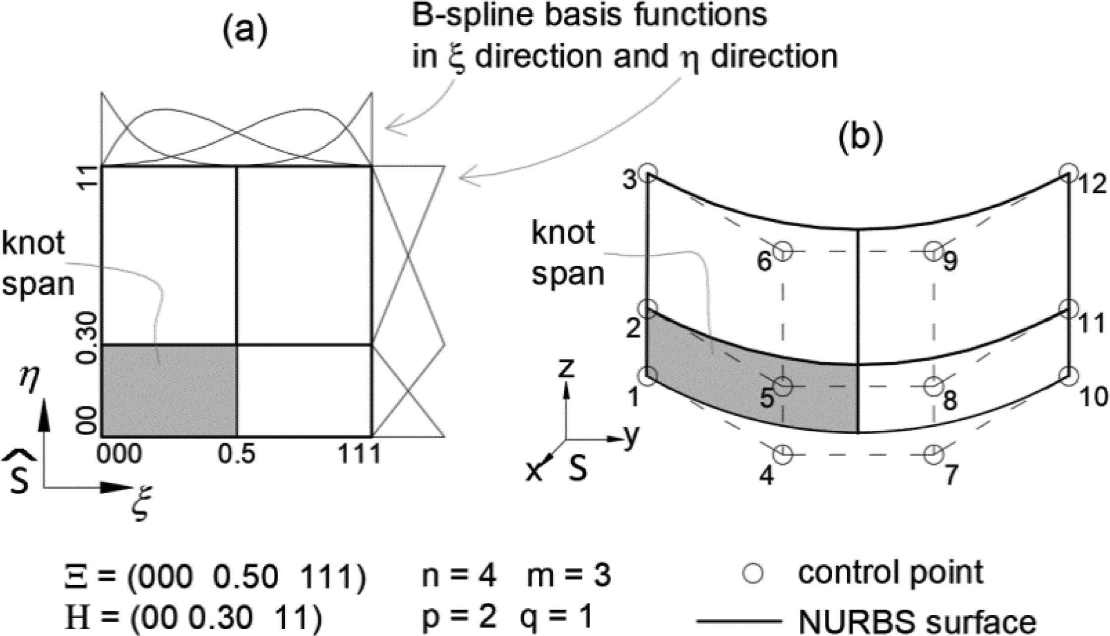
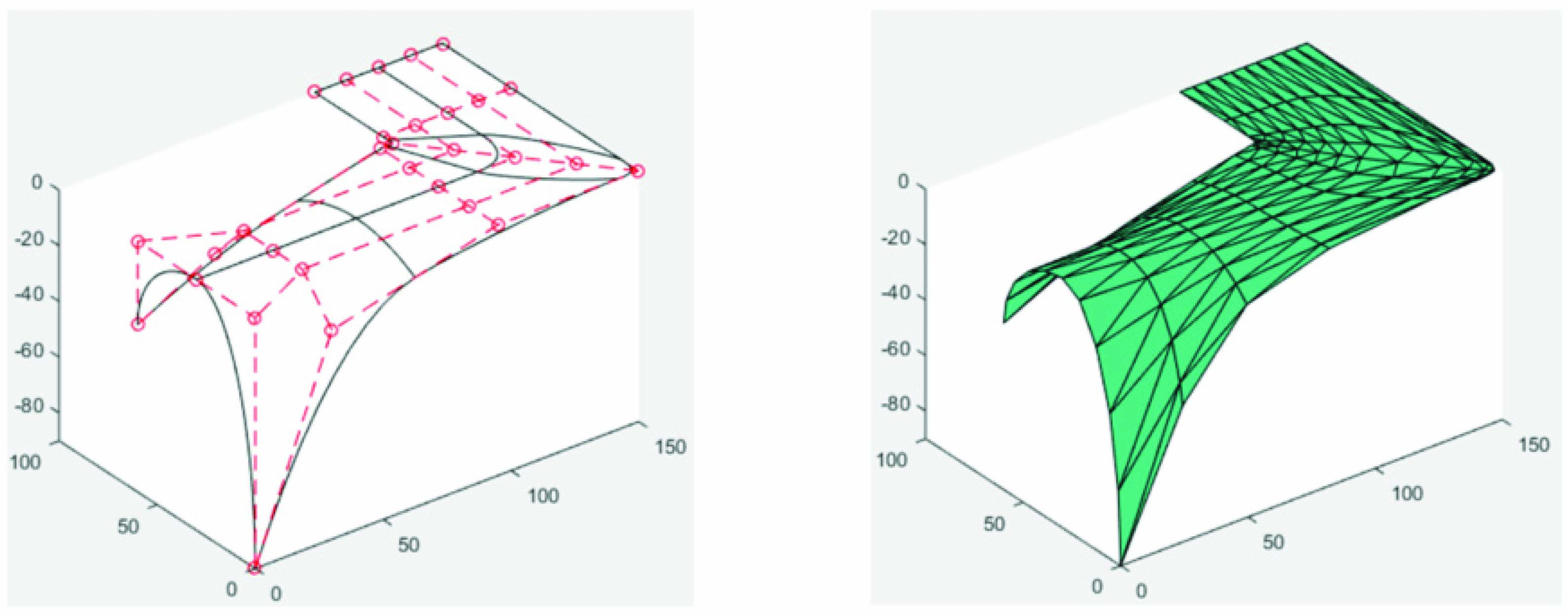
A NURBS entity (curve or surface) is defined in both the parameter and physical spaces. The number of dimensions for the parameter and physical spaces are $c$ and $d$ respectively, with $c<d$. For curves $c=1$ and for surfaces $c=2$. In this work we assume $d=3$. Figure 1 shows one NURBS surface example.

Figure 1 NURBS surface parameter (a) and physical (b) spaces.

NURBS entities are the evolution of Bézier entities [27, 28] that are formed by linear combination of Bernštein polynomials [29]. NURBS entities have a set of control points whose coordinates in the physical space are defined by P and weights defined by w. Each control point has attached one NURBS basis function. Parametrization is given by knot vectors, with one knot vector per each parameter direction. The knot vector is a sequence of numbers $𝜩=\{{\xi }_1{\xi }_2\mathrm{\cdots }{\xi }_a\mathrm{\cdots }{\xi }_{n+p+1}\}$ with ${\xi }_i\le {\xi }_{i+1}$. The components of $𝜩$, called knots, are located in the parameter space. Stretches between knots are called knot spans. This work assumes knot values from 0 to 1 and open knot vectors, i.e. the first and last $p+1$ knots are repeated. The number of knots is equal to $p+n+1$, where p is de degree of the NURBS functions and n is the number of control points in the parameter direction. Table 1 shows the nomenclature used for curves and surfaces.

Table 1 NURBS nomenclature

		Surface
	Curve	Direction 1	Direction 2
Parameter coordinates	$\xi$	$\xi$	$\eta$
B-spline basis function	$N_i$	$N_i$	$M_j$
NURBS basis function	$R_i$	$R_{i,j}$
Number of control points	$n$	$n$	$m$
Degree	$p$	$p$	$q$
Knot vector	$𝜩$	$𝜩$	$H$
Physical space	$𝑪$	$𝑺$
Parameter space	$\widehat{𝑪}$	$\widehat{𝑺}$

A NURBS entity is generated by mapping ${ℝ}^c\to {ℝ}^d$ as detailed in Equations (1) and (2) for curves and surfaces respectively, where R are the NURBS basis functions.

$𝑪(\xi )$	$=$	${\displaystyle \sum _{i=1}^n}{R}_i^p(\xi ){𝑷}_i$	(1)
$𝑺(\xi ,\eta )$	$=$	${\displaystyle \sum _{i=1}^n}{\displaystyle \sum _{j=1}^m}{R}_{i,j}^{p,q}(\xi ,\eta ){𝑷}_{i,j}$	(2)

The NURBS basis functions are calculated as in (3) and (4).

$$R_i^p(\xi )=\frac{N_{i,p}(\xi )w_i}{{\sum }_{\widehat{i}=1}^n{N}_{\widehat{i},p}(\xi )w_{\widehat{i}}}$$

(3)

$$R_{i,j}^{p,q}(\xi ,\eta )=\frac{N_{i,p}(\xi )M_{j,q}(\eta )w_{i,j}}{{\sum }_{\widehat{i}=1}^n{\sum }_{\widehat{j}=1}^m{N}_{\widehat{i},p}(\xi )M_{\widehat{j},q}(\eta )w_{\widehat{i},\widehat{j}}}$$

(4)

B-spline functions N can be calculated with the Cox-De Boor iterative Equations (5) and (6) [30, 31]. Figure 1 (a) also includes the B-spline functions in both directions.

For zero degree ($p=0$):

$$N_{i,0}(\xi )=\{\begin{array}{cc}\hfill 1\hfill & \hfill \mathrm{if}{\xi }_i\le \xi <{\xi }_{i+1}\hfill \\ \hfill 0\hfill & \hfill \mathrm{otherwise}\hfill \end{array}$$

(5)

For degrees 1 and higher ($p>0$):

$$N_{i,p}=\frac{\xi -{\xi }_i}{{\xi }_{i+p}-{\xi }_i}{N}_{i,p-1}(\xi )+\frac{{\xi }_{i+p+1}-\xi }{{\xi }_{i+p+1}-{\xi }_{i+1}}{N}_{i+1,p-1}(\xi )$$

(6)

2.2 Length of Paths on NURBS

The physical path’s length for a NURBS curve between parameter coordinates ${\xi }^a$ and ${\xi }^b$, corresponding to physical coordinates ${𝒙}^a$ and ${𝒙}^b$, is given by the integral detailed in Equation (7).

$$L_{ab}={\int }_{{\xi }^a}^{{\xi }^b}\parallel 𝑪{,}_{\xi }\parallel d\xi$$

(7)

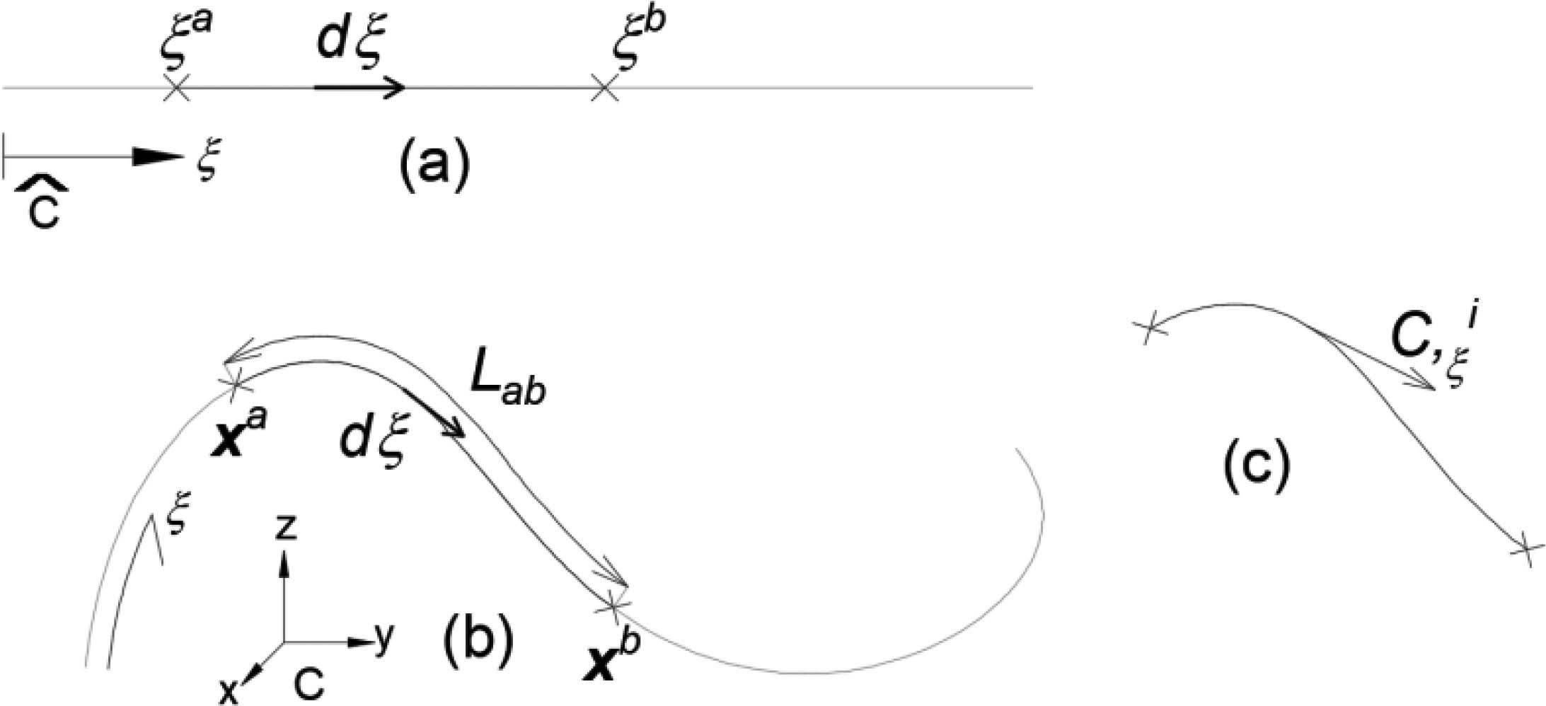
Where $\parallel 𝑪{,}_{\xi }\parallel$ is the norm of the curve derivative w.r.t. parameter coordinate $\xi$. See Figure 2 for clarity.

Figure 2 Curve path between $a$ and $b$ in parameter (a) and physical (b) spaces. Derivative at $i$th point (c).

The physical length of a path on a NURBS surface between parameter coordinates ${𝝃}^a$ to ${𝝃}^b$, that forms a $\theta$ angle w.r.t. the horizontal direction and corresponds to physical coordinates ${𝒙}^a$ and ${𝒙}^b$, is given by the integral of the $\theta$-directional derivative norm along the path as follows:

$$L_{ab}={\int }_{{𝝃}^a}^{{𝝃}^b}\parallel 𝑺{,}_{\lambda }\parallel d\lambda$$

(8)

Where $d\lambda$ represents an infinitesimal increment in the parameter domain with orientation $\theta$, and $𝑺{,}_{\lambda }$ is the $\theta$ - directional derivative, i.e. $𝑺{,}_{\lambda }={(Sx{,}_{\lambda },Sy{,}_{\lambda }Sz{,}_{\lambda })}^T$ that is computed as per Equation (9).

$$𝑺{,}_{\lambda }=𝑺{,}_{\xi }cos\theta +𝑺{,}_{\eta }sin\theta$$

(9)

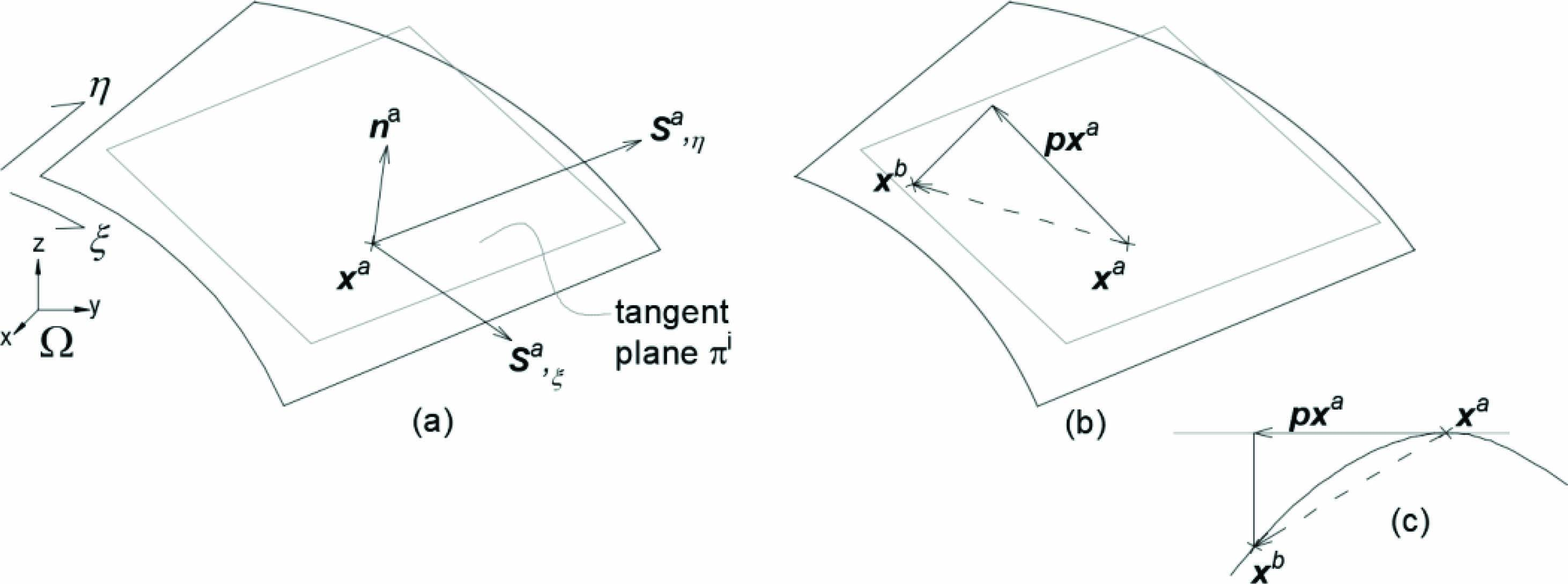
The distance $L_{ab}$ lies onto the surface (physical space) but the shortest distance between ${𝒙}^a$ and ${𝒙}^b$ might be less (see Figure 3(b)).

Figure 3 Surface path between $a$ and $b$ in parameter (a) and physical (b) spaces. Directional derivative at $i$th point (c).

We can generalize Equations (7) and (8) by calling $𝑯$ to the NURBS entity and $\mu$ to the parameter ($\xi ,𝝃$ or $\lambda$). Then these two expressions may be written as in Equation (10), with $h=\parallel 𝑯{,}_{\mu }\parallel$.

$$L_{ab}={\int }_{{\mu }^a}^{{\mu }^b}h𝑑\mu$$

(10)

2.3 Trapezoidal Rule for Path Lengths

The estimation of the path’s length by the trapezoidal rule is expressed as:

$$L_{ab}\approx \frac{1}{2}(h^b+h^a)\mathrm{\Delta }\mu$$

(11)

Under appropriate smoothness assumptions, there exists some point $\alpha$ in the integration interval such that the error is bounded, as expressed in Equation (12) [32], where $\mathrm{\Delta }\mu =({\mu }^b-{\mu }^a)$. Since the location $\alpha$ is unknown, in this work we will evaluate the error at the initial and final locations for the following interval:

$$E\le \frac{-1}{12}\parallel 𝑯{,}_{\mu }^{\alpha }{\parallel }^{\prime \prime }{(\mathrm{\Delta }\mu )}^3$$

(12)

The calculation of the derivatives $\parallel 𝑪{,}_{\xi }{\parallel }^{\prime \prime }$ and $\parallel 𝑺{,}_{\lambda }{\parallel }^{\prime \prime }$ is detailed in Appendix A. The error is expressed as percentage of the path’s length:

$$Ep\le 100\frac{E}{L}$$

(13)

where $E$ is the absolute value of the error, computed as in Equation (12) and $L$ is the estimated physical length of the path as in Equation (11).

2.4 Path Parameter Increment Corresponding to a Physical Length (PPI)

Let $L_{ab}$ be the length of a path that lies in the physical space of a NURBS entity whose end points are a and b. Let c be a third point along the path trajectory, either between the end points or beyond b (see Figure 4). The Path Parameter Increment procedure (PPI) presented in this section finds the parameter coordinate b (${\mu }^b$), assuming that the physical coordinates of the three points and the parameter coordinates of a and c (${\mu }^a$ and ${\mu }^c$) are known.

Figure 4 Path with points a, b and c in physical (a) and parameter (b) spaces. Line in the $h$-$\Delta \mu$ plane (c).

The trapezoidal rule between a and b is written as in Equation (11) with $\mathrm{\Delta }\mu$ and $h^b$ being unknowns in this case. To compute $\mathrm{\Delta }\mu$ we use the third point c, whose derivative norm $h^c$ lies on the line $h$-$\Delta \mu$, as shown in Figure 4(c). Equation (14) is used, where it was assumed that $\Delta \mu =0$ coincides with the $h^a$ location:

$$h(\Delta \mu )=(\frac{h^c-h^a}{{\mu }^c-{\mu }^a})\Delta \mu +h^a$$

(14)

Substituting $h^b$ in Equation (11) with the right-hand side of Equation (14), we arrive to the quadratic equation for $\Delta \mu$, Equation (15), where $m=\left(\frac{h^c-h^a}{{\mu }^c-{\mu }^a}\right)$. Among the two possible roots, the non-negative and within, or closest to, the interval $({\mu }^a,{\mu }^c)$ corresponds to the searched increment $\mathrm{\Delta }{\mu }^{*}$.

$$\Delta {\mu }^{2}m+\Delta \mu 2h^a-2L_{ab}=0$$

(15)

Then, the coordinate ${\mu }^b$ is given by:

$${\mu }^b={\mu }^a+\mathrm{\Delta }{\mu }^{*}$$

(16)

2.5 Orientation of a Surface Tangent Vector in the Parameter Space

Let ${𝒗}^k$ be a tangent vector to a surface at point $k$ in the physical space, the calculation of its orientation in the surface parameter space ($\theta$) will be presented in this section. ${𝒗}^k$ is a linear combination of main derivatives as shown in Equation (17) (see Figure 5). Coefficients $c$ and $s$ are shortcuts to “$\mathcal{𝒞}cos\theta$” and “$\mathcal{𝒞}sin\theta$”, respectively, with $\mathcal{𝒞}$ being an unknown constant.

$$c𝑺{,}_{\xi }^k+s𝑺{,}_{\eta }^k={𝒗}^k$$

(17)

Figure 5 Vector ${𝒗}^k$ in in physical space and its orientation in the parameter space.

To compute the orientation $\theta$, the derivatives $𝑺{,}_{\xi }^k$ and $𝑺{,}_{\eta }^k$ are firstly calculated, then $c$ and $s$ are obtained from the system of Equations (17). Finally, $\theta$ is calculated as in the following equation:

$$\theta =atan\left(\frac{s}{c}\right)$$

(18)

3 Preliminaries

3.1 Pattern Space

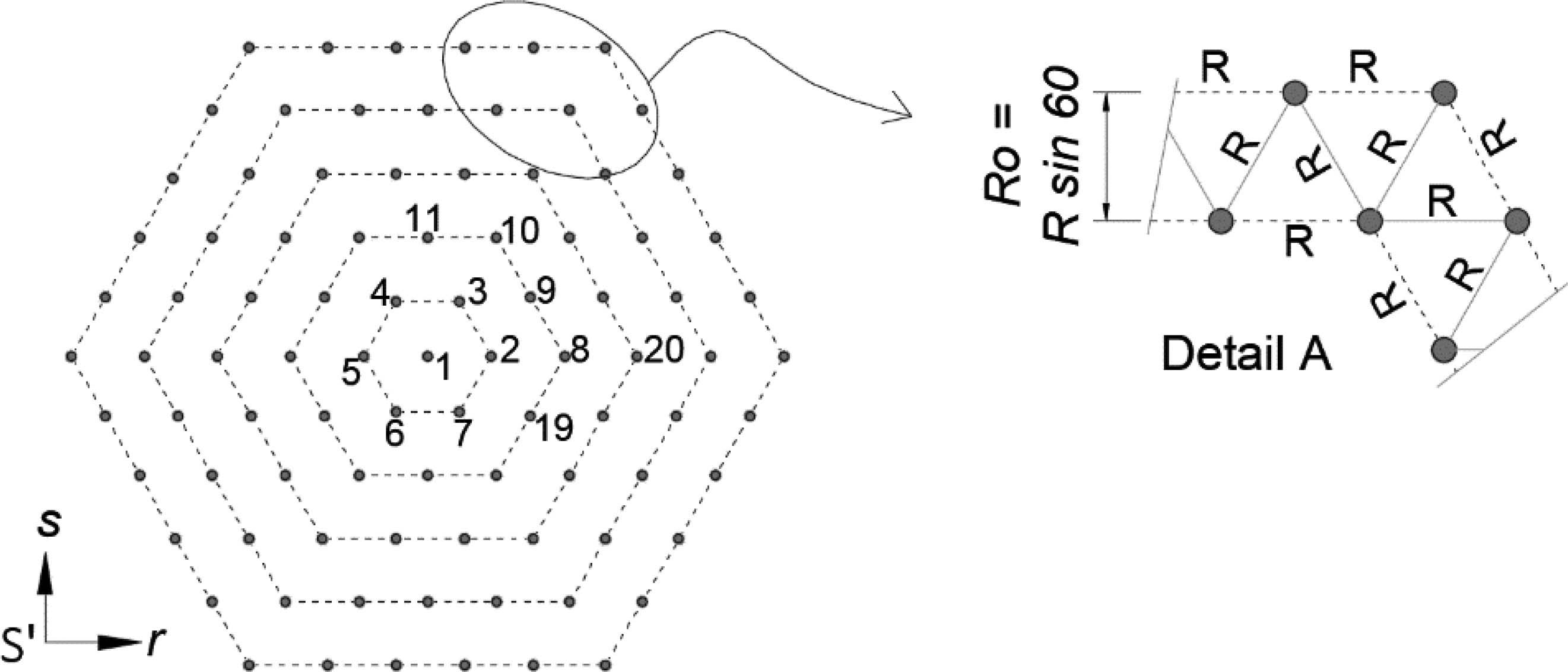
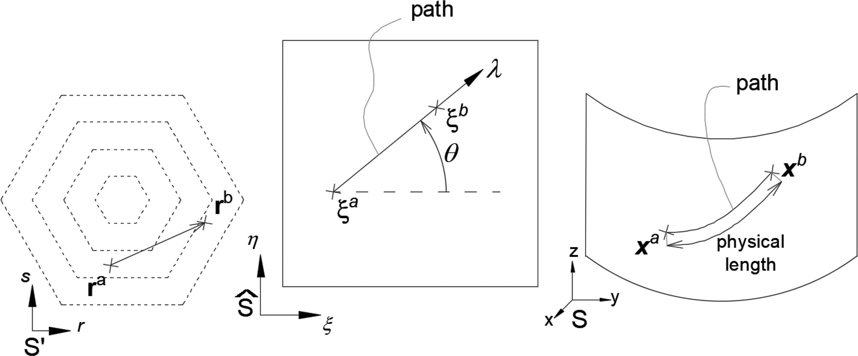
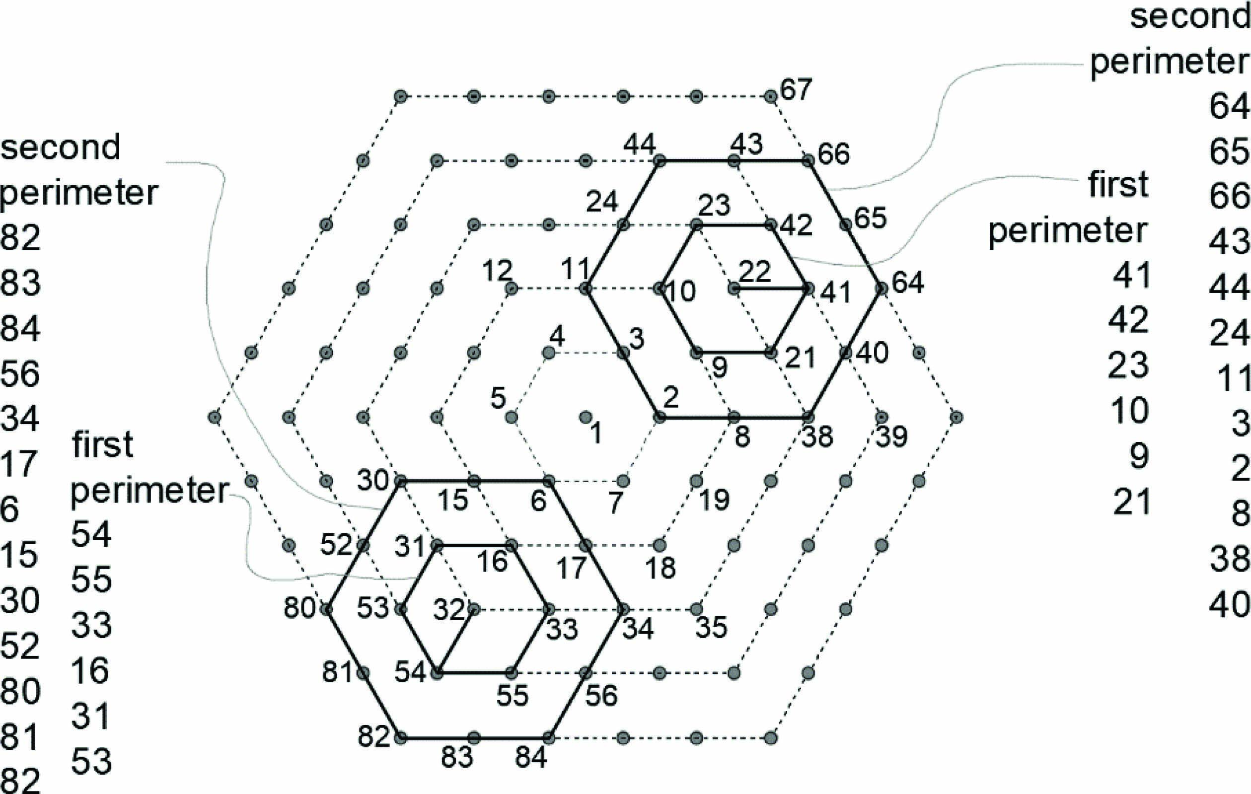
In this work we introduce a new 2D space, named pattern space (${\mathrm{S}}^{\prime }$), as a set of vertexes lying on a number of concentric regular hexagons separated by the distance $R_o=Rsin60$. Vertexes are equally spaced at $R$. Due to the regular hexagonal arrangement, these vertexes form an isotropic triangulation in this space, see Figure 6.

The centre of the hexagons is located at origin $(0,0)$. Hexagon one is the smallest with six vertexes and the rest of the hexagons grow concentrically with 12, 18, etc vertexes. Vertexes are numbered: the central is the first and the numbering increases for each hexagon that is generated. Inside one hexagon, numbers start at the right-hand side corner and move counter-clockwise (Figure 6 shows some vertex numbers). Considering this additional new space for the hexagons (pattern space), three spaces are now involved for each surface: pattern, parameter and physical spaces.

Figure 6 Pattern space with five contours (dashed lines). Dots represent vertexes.

3.2 A Whole View: The QIT Algorithm

The Quasi-Isotropic initial Triangulation (QIT) algorithm purpose is to mesh a set of contiguous NURBS surfaces, each of them bounded by four edge curves, with conformal triangulations between contiguous surfaces and with a high degree of isotropy.

The strategy is to obtain the image of the pattern space vertexes onto the surface physical space, which leads naturally to a quasi-isotropic mesh given the pattern space arrangement indicated in Section 3.1. The target distance between vertexes is called $R$ and is introduced by the user.

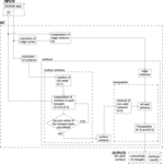
Figure 7 details the flowchart for the process that is briefed in this section. The algorithm provides the vertexes coordinates and their relationship in the triangulation (the connectivity matrix). The inputs required for the QIT algorithm are:

– Target triangles edge distance $(R)$: this is the distance that ideally all the triangles edges should have in the physical surface.

– Threshold distance in the physical space from the surface edges to discriminate surface vertexes.

– Tolerance for the error, in percentage, when computing path lengths (recall Section 2.3).

– NURBS original data of the surfaces.

Figure 7 QIT algorithm flowchart. Related sections of the paper are in curved brackets.

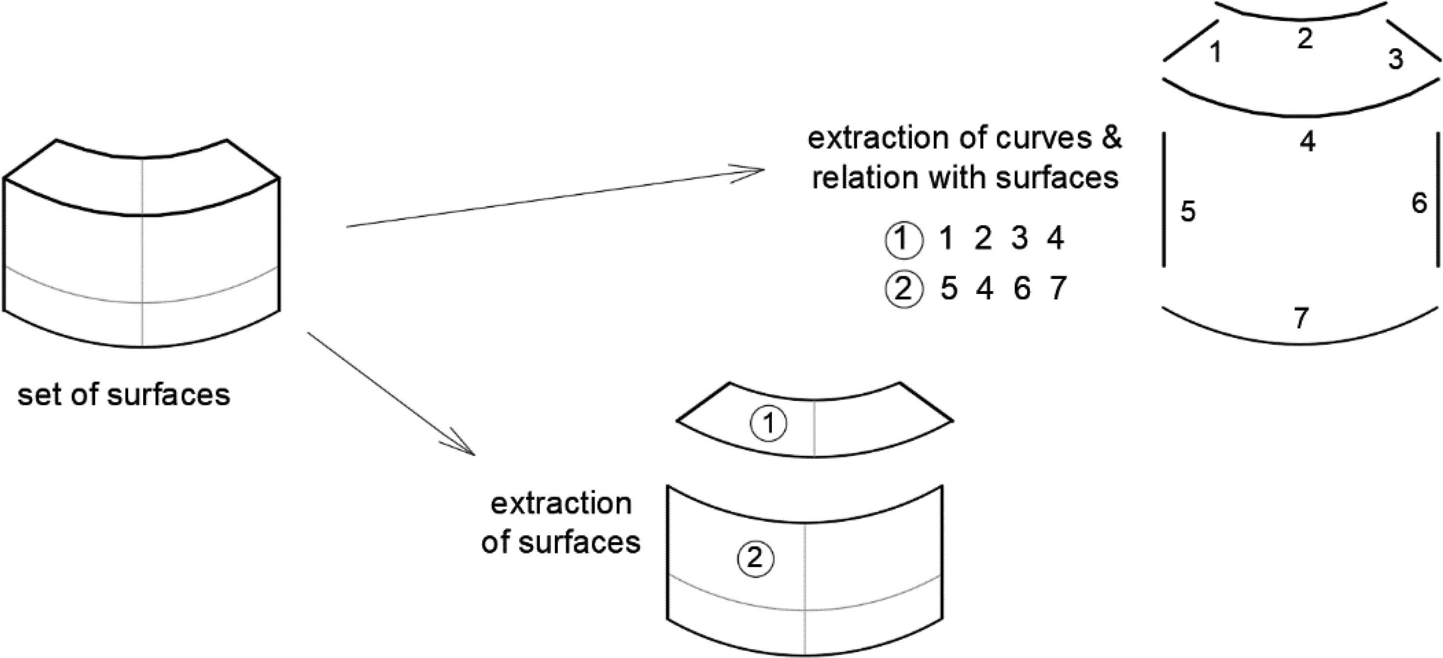
Edges between two adjacent surfaces produce duplicated curves, one per surface. In order to compute the vertexes in both curves with the same coordinates and achieve conformity between them, they must be considered as a single curve instead (see Figure 8). All curves are extracted and those duplicated are merged into one. Their vertexes are obtained according to the $R$ distance, these are called edge vertexes. Section 4 delivers more details of this process.

Figure 8 Extraction of surfaces and curves and their relationship.

Each surface is triangulated separately: the surface vertexes are calculated, the corresponding edge vertexes are added and all vertexes are triangulated. Surface vertexes calculation is outlined in Figure 9. The surface parameter space is discretized in a mesh called dS-mesh (Section 5.1). The first vertex is set at mid location and the rest of the vertexes are calculated in a 2D hexagonal wave propagation manner. Propagation stops at the hexagon with no vertexes computed (see Sections 5.4 and 5.5). This procedure links vertexes in pattern space with their image in the physical space using the parameter space in between (see Sections 5.2 and 5.3).

Figure 9 Computation of surface vertexes.

The advancing front algorithm is divergent in the physical space, therefore it is also in the parameter space (we assume the Jacobian of the NURBS mapping to be strictly positive). That divergence is necessary because it avoids front collisions.

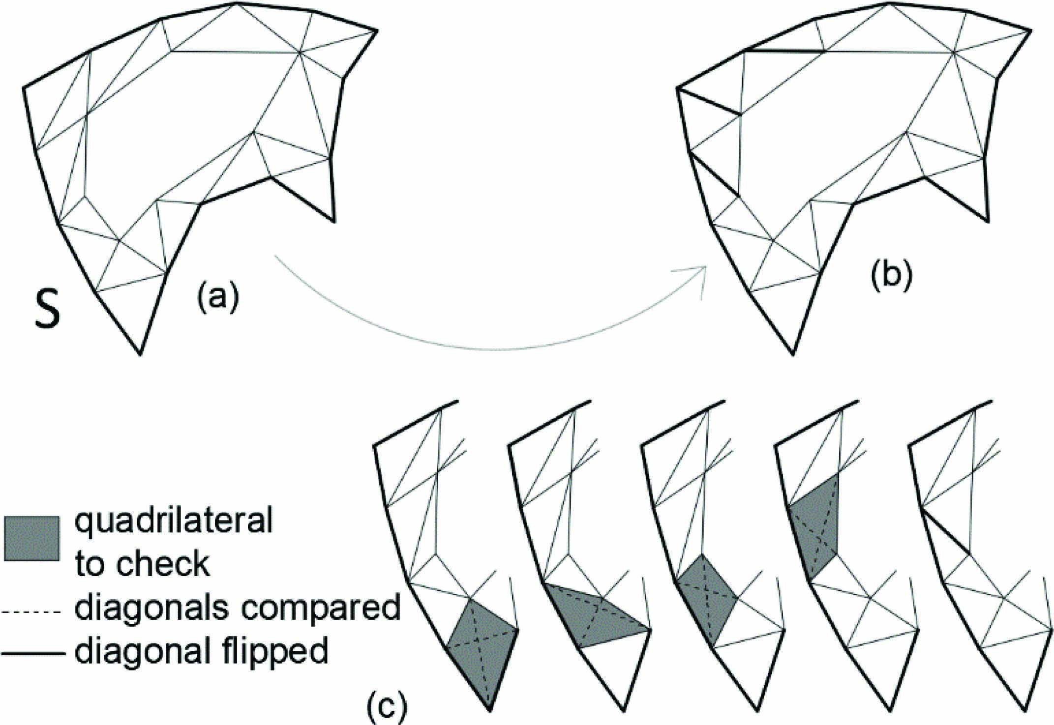
Previous to triangulation, surface vertexes outside the parameter limits are removed as well as those that are too close to the limits, since they would generate highly distorted triangles (see Section 6.2). The remaining vertexes are called valid. Delaunay triangulation is carried out in the pattern space considering both, edge and valid surface vertexes (see Section 6.3). Finally, the triangles at the edges of the surface might be improved by edge flipping, as shown in Section 6.4. The triangulation process is illustrated in Figure 10.

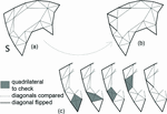
Figure 10 Triangulation in the pattern space (a), image in the physical space (b) and improvement of edges (c).

3.3 Conventions and Definitions

Coordinates in the pattern, parameter and physical spaces are expressed as $𝒓=(r,s),𝝃=(\xi ,\eta )$ and $𝒙=(x,y,z)$, respectively. Coordinates at a specific point $a$ are written with $a$ as superscript, e.g. ${𝒓}^a$. The expression vertex calculation refers to the calculation of the vertex coordinates.

The definitions listed below are used within the next sections. Figure 11 provides some examples of them for clarity.

Figure 11 Basic definitions used in the algorithm in pattern, parameter and physical spaces.

– Path: straight line between two points in the parameter space, that has an image in the surface space, which is not straight in general.

– $\theta$ orientation: angle between a path and the horizontal axis in the parameter space.

– $\lambda$: surface parameter coordinate with orientation $\theta$.

– Path length: length of a path in the physical space (in general it is not the shortest).

– Edge vertex: vertex computed on edge curves.

– Surface vertex: vertex computed on the surface.

– Main derivatives: surface derivatives w.r.t. parameter directions $\xi$ and $\eta$.

4 Vertexes of Edge Curves

The computation of vertexes for edge curves is explained in this section. The first step is a parameter space discretization into a dC-mesh in order to control the error of the estimated path lengths.

4.1 Discretization of the Parameter Space. The dC-mesh

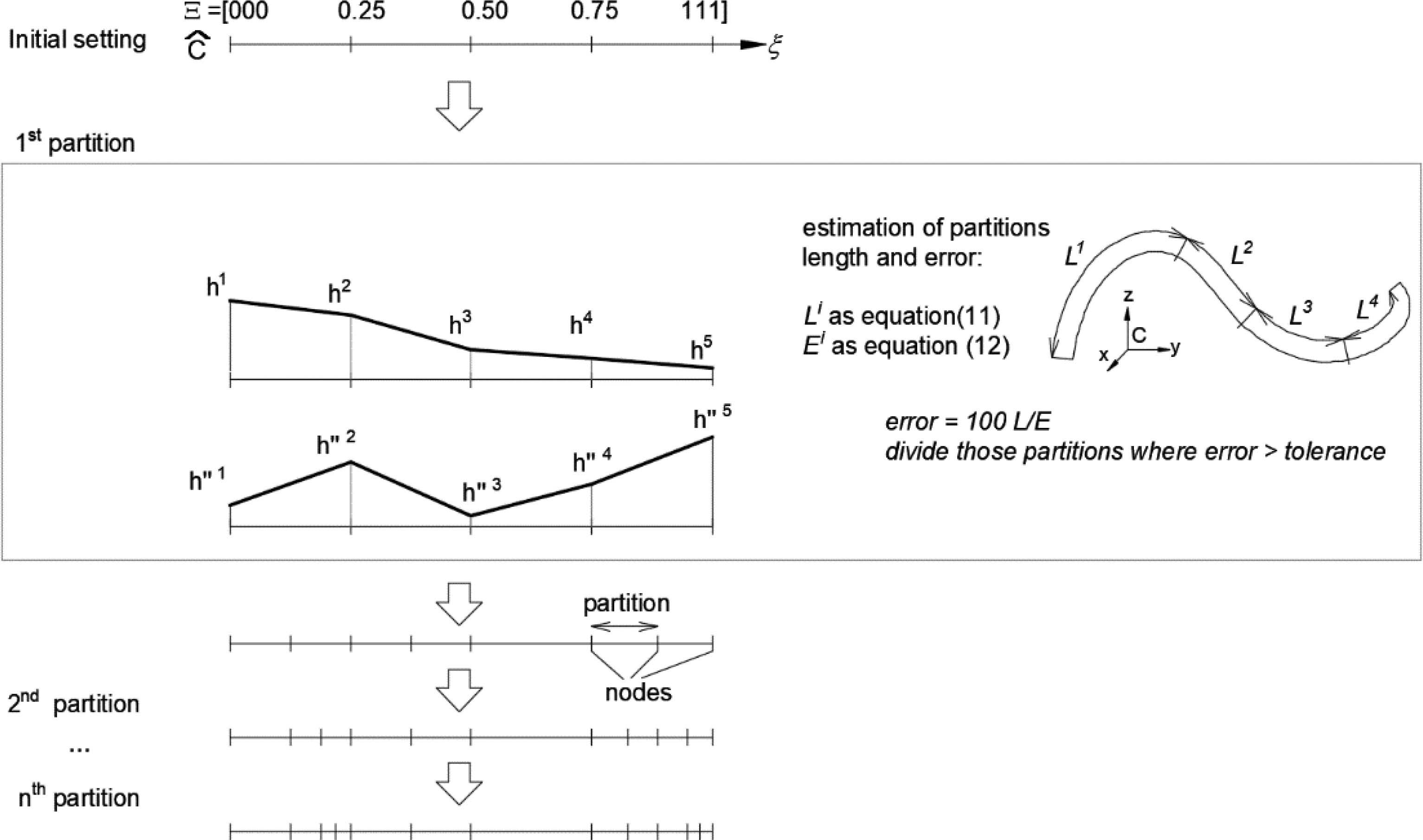
The dC-mesh is obtained by iterative division of the parameter space so that the error $E_p$ from Equation (13) can be reduced for a path length estimation below a prescribed tolerance. We refer to the norm of the curve derivative $\parallel 𝑪{,}_{\xi }\parallel$ by $h$ and its second derivative $\parallel 𝑪{,}_{\xi }{\parallel }^{\prime \prime }$ by $h^{\prime \prime }$ (see Appendix A for the calculation of $h^{\prime \prime }$).

Initially, dC-mesh partitions coincide with non-void knot vector spans. Then, within each partition, the $E_p$ is computed and, in case it is greater than a prescribed tolerance, the element is halved. This iterative process ends whenever there is no partition with an error greater than the prescribed tolerance. The extremities of the partitions are called nodes. Figure 12 provides one example. To compute the partitions length and error, $h$ and $h^{\prime \prime }$ are calculated for each node (recall Equations (11) and (12)).

Figure 12 dC-mesh division process with first step detailed.

The error at some locations might be greater than the tolerance since the location $\alpha$, introduced in (12), is the initial or final node of the partition, whichever maximizes the error, but there might exist an intermediate value that leads to a higher error. In spite of this risk, results are satisfactory (refer to Section 7).

4.2 Edge Vertexes Calculation

To calculate the edge vertexes, the accumulated physical length up to each dC-mesh node, called $Lacc$, is estimated by using the trapezoidal rule from Equation (11) applied to each partition, see Figure 13. The total estimated length of the curve is $L_{acc}^{end}$ and the accumulated length up to the previous node is $Lac{c}^{prev}$.

Figure 13 Computation of accumulated length to each dC-mesh node.

The target physical spacing between vertexes is not exactly $R$ but it is re-calculated to ensure that the resultant vertexes are equally spaced. The updated spacing is called $Rc$ and is obtained as $Rc=L_{acc}^{end}/NS$, where $NS=round(L_{acc}^{end}/R)$ is the number of required segments between vertexes.

Accumulated target distances ($Ra$) are then sequentially searched. $Ra$ initially is set equal to $Rc$ and increases by $Rc$ in each step. The search first finds which partition of the dC-mesh contains $Ra$, using the accumulated physical lengths $Lacc$. Then, it estimates the parameter coordinate increment $\mathrm{\Delta }\xi$ within that partition in order to achieve the distance $L=R_a-Lac{c}^{prev}$ by using the PPI algorithm from Section 2.5. See one example in Figure 14.

Figure 14 Example for the calculation of the seventh vertex.

The edge vertexes in the surface parameter space, required for triangulation (see Section 6), are computed by using point projection techniques [34].

5 Surface Vertexes

For the calculation of surface vertexes the surface must first be discretized into a dS-mesh (Section 5.1). Sections 5.2 and 5.3 explain the two main algorithms used repeatedly in Sections 5.4 and 5.5 for the computation of the surface vertexes.

5.1 Discretization of the Parameter Space. The dS-mesh

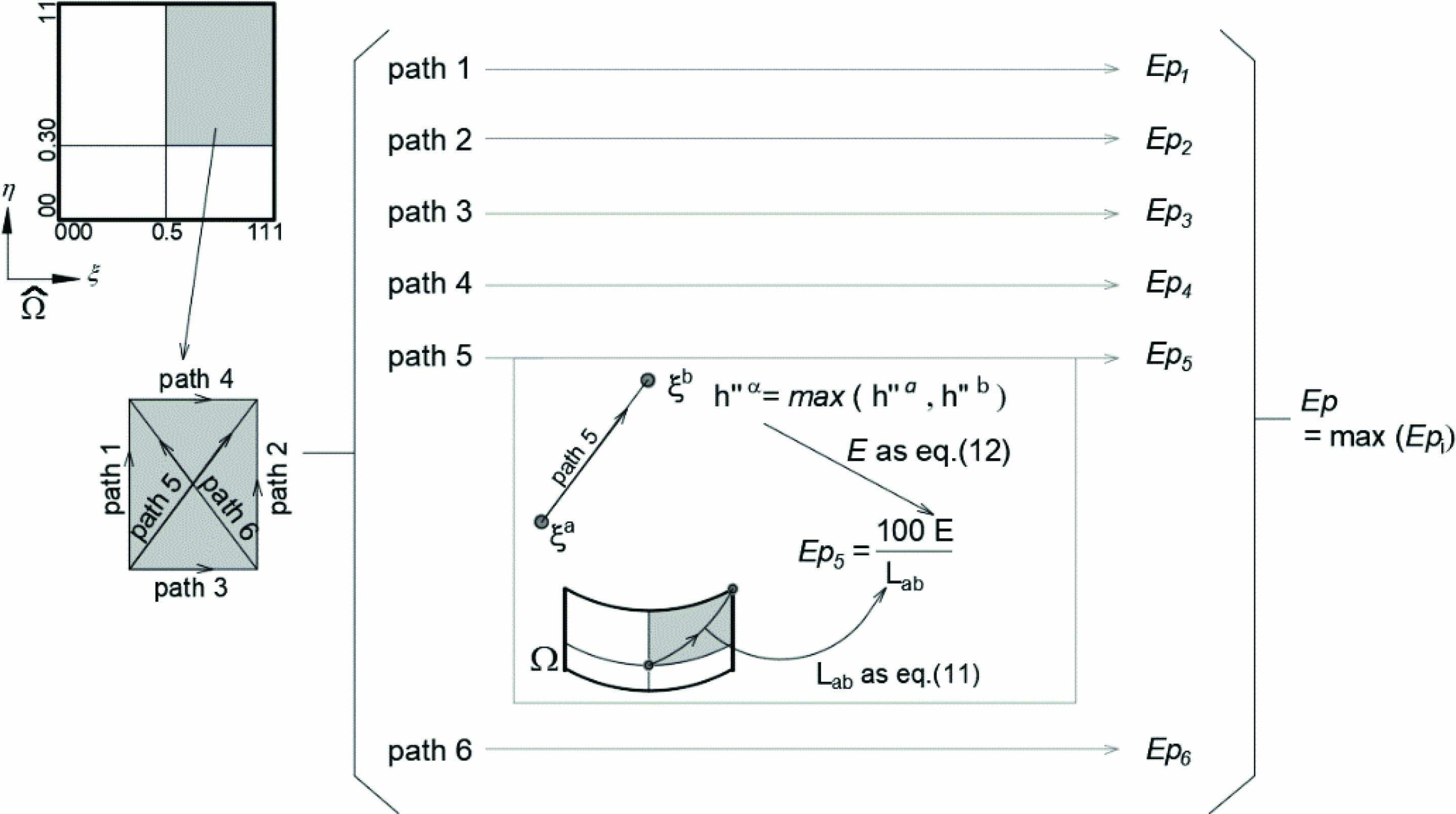
The dS-mesh is obtained by iterative partition of the parameter space. Resultant rectangular partitions must be small enough such that the error in Equations (12) and (13) for any patch length remains below a prescribed tolerance.

Six representative paths were selected within each partition of the dS-mesh, they are the four edges and its two diagonals. The partition error is the maximum error amongst these six paths. The second derivative $\parallel 𝑺{,}_{\lambda }^{\alpha }{\parallel }^{\prime \prime }$, selected for error calculation (12), must be the maximum amongst the two end points of the corresponding path. The calculation of these derivatives is detailed in Appendix A. Figure 15 shows one example, with the fifth path detailed and where $\parallel 𝑺{,}_{\lambda }{\parallel }^{\prime \prime }$ is called $h^{\prime \prime }$ for simplicity.

Figure 15 Error measurement in one partition of the dS-mesh.

Initially, partitions are the non-void knot spans. Error ($E_p$) is evaluated for each partition, which is divided into four rectangles if such error is greater than the tolerance. The division process ends whenever the error is smaller than the prescribed tolerance in all partitions.

Once the partitions are generated, the dS-mesh is extended beyond the surface parameter limits with so-called perimeter partitions and corner partitions. The main derivatives on these partitions are merely an extension of the derivatives at the edge limits. These partitions are semi-infinite, i.e. one end coincides with the surface parameter limit and the opposite goes to the infinite. This extension will be relevant in Section 5.4. The whole process is depicted in Figure 16.

Figure 16 dS-mesh generation: initial setting, partition and extension with perimeter and corner partitions.

It is possible to find locations where the error is greater than the tolerance because the location $\alpha$ introduced in Equation (12) lies at the start or at the end of the path (recall Figure 15) but there might exist an intermediate value that leads to a higher error. In addition, only six orientations for the paths are analysed event though there are infinite possibilities. In spite of this risk, results are satisfactory (refer to Section 7).

5.2 End Parameter Position of a Path Given its Physical Length (EPP)

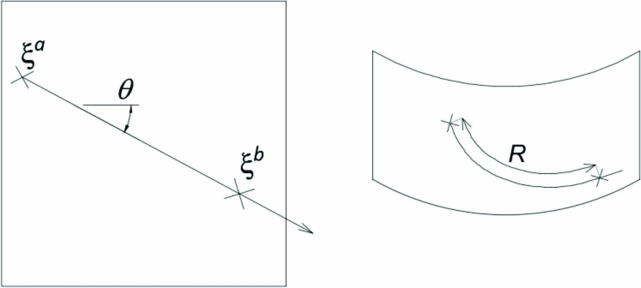
This section explains the End Parameter Position procedure (EPP) that estimates the end location ${𝝃}^b$ of a path whose initial point coordinates ${𝝃}^a$, orientation $\theta$ and physical length are known a priori. The physical length is called target length and it is denoted by R, as shown in Figure 17.

Figure 17 Path in parameter (left) and physical (right) spaces. The position ${𝝃}^b$ is the output of the EPP algorithm.

A semi-infinite line, starting at ${𝝃}^a$ and with orientation $\theta$ is defined (see Figure 18). The procedure is to move along this line computing at each time its intersection with dS-mesh edges and calculating the segment physical length by using the trapezoidal rule of Equation (11). The $\theta$-directional derivatives required for Equation (11) can be estimated as shown in Appendix B. When the accumulated length of the segments goes beyond the target $R$, the parameter coordinate ${𝝃}^b$ is searched by PPI within the current segment (see Section 2.5). Some examples are illustrated in Figure 19.

Figure 18 Estimation of different path increments to achieve the physical target distance $R$. Above represents the parameter space, with grey hatching the partition of dS-mesh involved. Below it is detailed the path in the physical space.

One special case happens when the ray passes the surface parameter limits and does not intersect any more partition edges. For this situation, the second trial point c for PPI cannot be computed from the intersection with the dS-mesh. Instead, it is obtained by adding a certain distance along the $\theta$ direction. In this work, the diagonal length of the surface parameter space ($u_{diag}$) is used for that effect. Figure 19 shows two examples representing this particular case.

Figure 19 Examples of application of the EPP for some particular cases.

5.3 Intersection of Two Arcs in Physical Space (AIP)

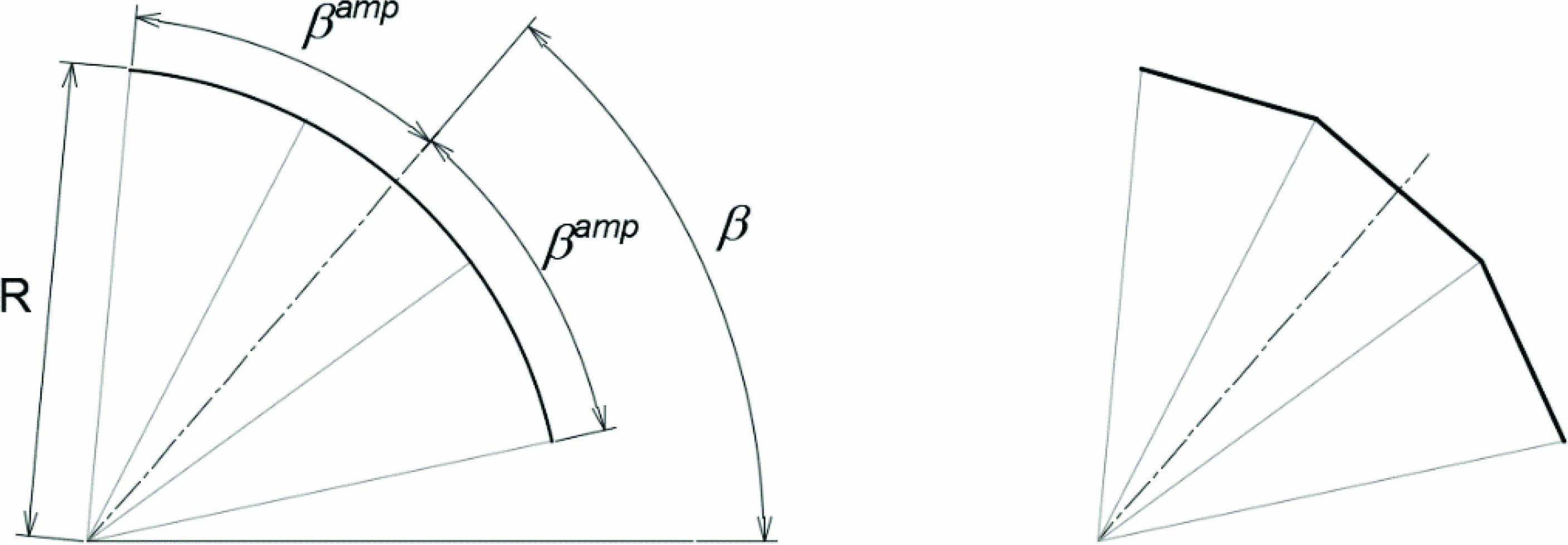
In this section a procedure called Arcs Intersection in Physical space (AIP) will compute the intersection (point $c$) of two arcs, $a$ and $b$, that lie on the physical space of the surface. Let us define one arc, onto the surface physical space centred at ${𝒙}^a$, by its radius ($R$), trial angle ($\beta$) and amplitude (${\beta }^{amp}$), in this work ${\beta }^{amp}=15$ degrees. The trial angle is the orientation of the arc bisector and the total arc angle is twice the amplitude (see Figure 20).

Figure 20 Definition of arc and discretization into three lines.

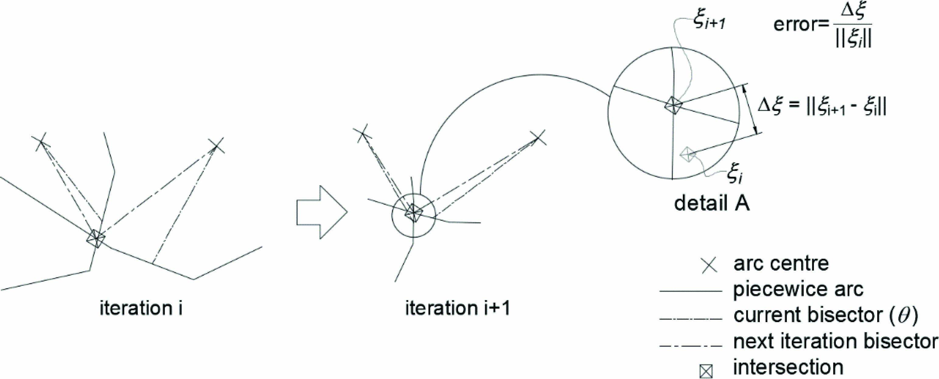
To find the intersection, arcs are first discretized in a number of lines ($NL$), as shown in Figure 20 at the right. Hence, the number of points to compute per arc is $NL+1$ (in this work $NL=3$). Due to this discretization procedure, a number of iterations is required to find the intersection point c. The iterative process ends when the difference between two consecutive intersections is less than a pre-established tolerance (in this work it is 1.0%). After each iteration, the trial angles are re-oriented to the updated intersection and the amplitudes are also adjusted accordingly. The rest of this sub-section has two parts, one to explain the calculation of the end-points of the arc lines and another to describe the iterative process.

Discretization of arcs:
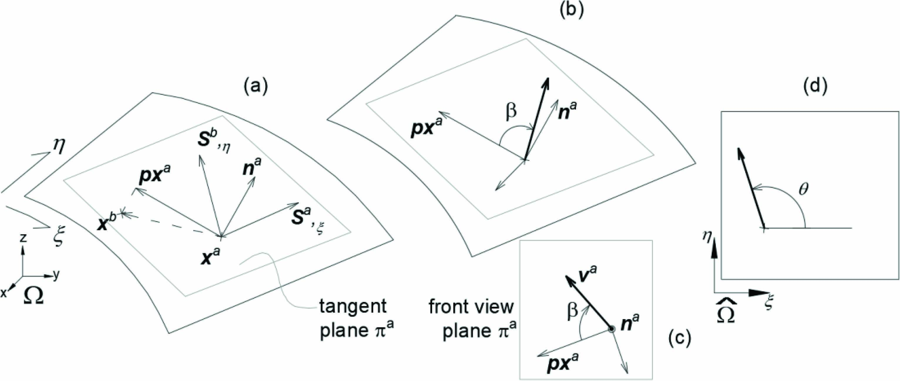
Let us define ${\pi }^a$ as the tangent plane to the surface at location ${𝒙}^a$, and $𝒑{𝒙}^a$ as the vector projected from vector ${𝒙}^b\mathbf{-}{𝒙}^a$ onto ${\pi }^a$, with all of these vectors represented in the physical space (Figure 21).

Figure 21 Tangent plane obtained by cross product of the derivatives to the surface (a). Projected vector $𝒑{𝒙}^a$ onto the ${\pi }^a$ plane (b). Front view of the projection’s procedure at the right-bottom (c).

The trial angle ${\beta }^a$ is measured from vector $𝒑{𝒙}^a$ as shown in Figure 22. The value of ${\beta }^a$ for the first iteration is selected in the pattern space by using relative positions between pattern coordinates of points ${𝒓}^a$, ${𝒓}^b$ and ${𝒓}^c$. Their values are typically around -60 and +60 degrees for ${\beta }^a$ and ${\beta }^b$, respectively, except for the first hexagon (see Section 5.4). The angles for the arc points vary from $\beta ^a{}_1={\beta }^a-{\beta }^{amp}$ to $\beta ^a{}_4={\beta }^a+{\beta }^{amp}$, with steps $\mathrm{\Delta }\beta =2{\beta }^{amp}/NL$, all within the ${\pi }^a$ plane.

Figure 22 Arc angles in the ${\pi }^a$ plane (a) and their counterparts in the parameter space (b). Trial angle and angles for points 1 and 4 are also indicated.

Points for the discretized arcs are computed by the EPP algorithm from Section 5.2, whose inputs needed are the location ${𝝃}^a$, the target distance $R^a$ and the orientation $\theta$ in parameter space. This angle corresponds to $\beta$, but defined w.r.t. the horizontal axis in the parameter space. The procedure to find $\theta$ from $\beta$ is depicted in Figure 23 and its steps are explained below:

Figure 23 Calculation of angle $\theta$ correspondent to the $\beta$ angle. Computation of the ${\pi }^a$ plane and projected vector $𝒑{𝒙}^a$ (a); local base ${𝑩}^a$ (b); vector with $\beta$ angle ${𝒗}^a$ (c); corresponding angle $\theta$ in the parameter space (d).

– Compute the tangent plane ${\pi }^a$ in the physical space. The normal vector to the plane is given by ${𝒏}^{𝒂}\mathbf{=}𝑺{,}_{\xi }^a\times 𝑺{,}_{\eta }^a$ (for the computation of the derivatives see Appendix B).

– Find $𝒑{𝒙}^a$: the projection of ${𝒙}_b^a$ onto ${\pi }^a$ (for arc $b$ use ${𝒙}_a^b$).

– Form local base ${𝑩}^a$ with vectors ${𝒏}^{𝒂}$, $𝒑{𝒙}^a$ and $𝒘$. Note that $𝒘\mathbf{=}{𝒏}^{𝒂}\times 𝒑{𝒙}^a$.

– Compute vector ${𝝂}^a$ contained in plane ${\pi }^a$ that forms $\beta$ degrees with $𝒑{𝒙}^a$. This step involves computing vector ${𝒗}^{a{}^{\mathbf{\prime }}}$ in the local base ${𝑩}^a$ (at $\beta$ degrees from $𝒑{𝒙}^a$) and transforming to the global coordinate system to obtain ${𝝂}^a$.

– Obtain $\theta$, which is the orientation of ${𝒗}^a$ referred to the horizontal axis in the parameter space, as described in Section 2.5.

The above-mentioned process is applied to the points of the arc for each iteration. The arc points obtained are equally spaced in the physical space but in the parameter space they can be distorted depending on the parametrization procedure used.

Iterative process:
Once the a and b arcs are discretized, the intersection of their lines can be calculated. The result is then compared against the previous intersection and, if it is greater than a threshold (1% in this work), arcs are re-defined and discretized again, and the intersection is re-calculated. If the difference is less than tolerance, then the process ends and the latest intersection is the one assumed valid.

After each iteration the trial angles are re-oriented to the latest computed intersection. The closer the initial trial angles (${\beta }^a$ and ${\beta }^b$) are to the final answer the smaller number of iterations are required. Since their initial values are taken from the pattern space, they are very close to the final answer and the number of iterations are typically equal or less than three. In addition, the pattern space is used to know the side that ${𝝃}^c$ must hold w.r.t. the vector from ${𝝃}^a$ to ${𝝃}^b$ (${𝝃}_b^a$) via the cross product ${𝒓}_b^a\times {𝒓}_c^a$. If the third component of this cross product is positive, then ${𝝃}^c$ must lie at the left-hand side of ${𝝃}_b^a$, otherwise it must lie at the right-hand side.

Four cases are possible to happen during the iterative process:

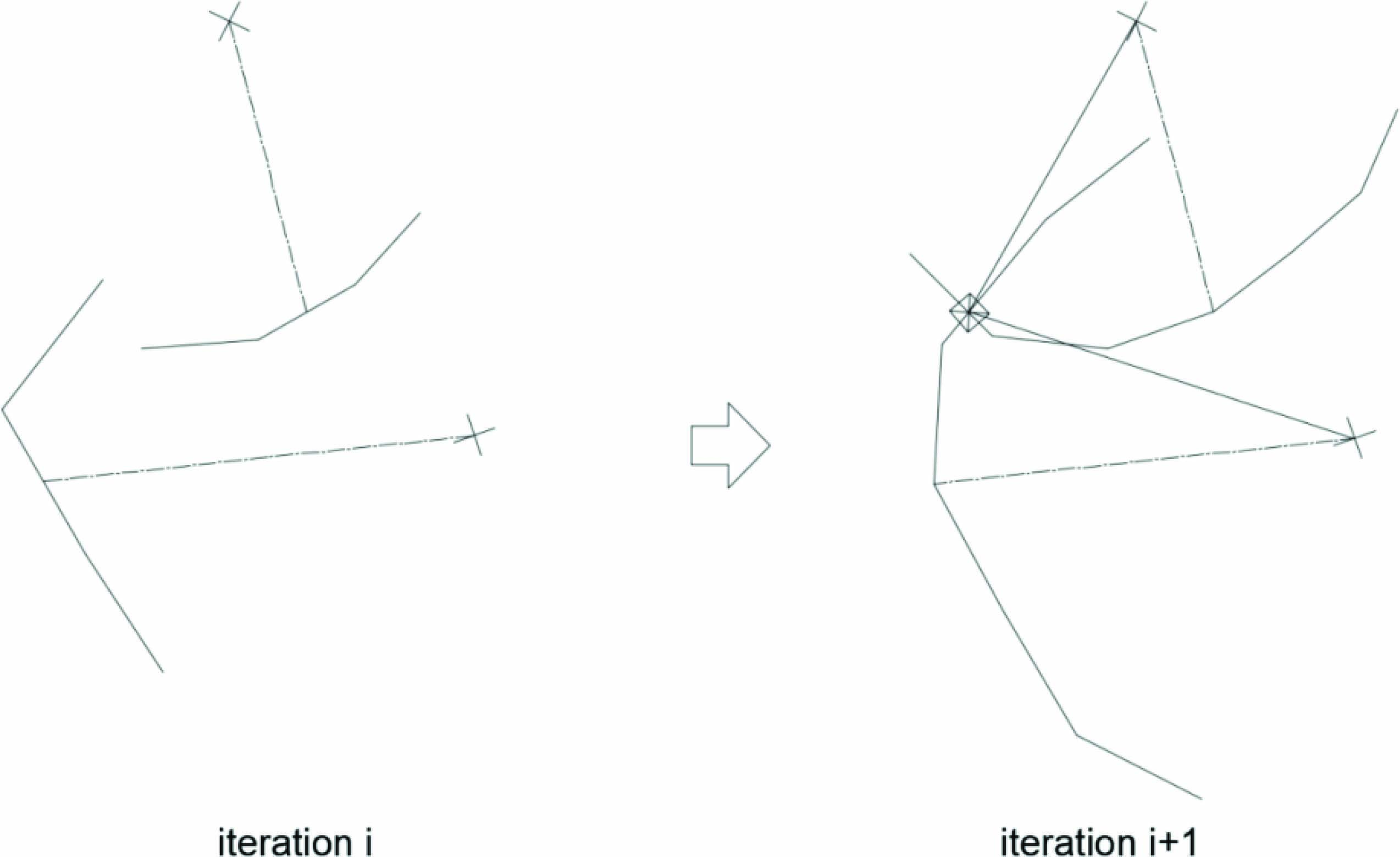
– Case A: intersection is found and it is in the correct side. If the error is greater than the tolerance then the next iteration is prepared: trial angles are reoriented to the updated intersection and arc amplitudes are reduced after dividing by $NL$. See Figure 24.

– Case B: intersection is found but it is located on the wrong side. The angle amplitude is then doubled, see Figure 25.

– Case C: no intersection is found. Both the angle amplitude and the number of segments per arc ($NL$) are doubled up for the next iteration, see Figure 26.

– Case D: the intersection was found previously but it was lost in the current iteration. The angle amplitude is then doubled for the next iteration.

Figure 24 AIP case A in the parameter space.

Figure 25 AIP case B in the parameter space. The pattern space is also shown for the ith iteration.

Figure 26 AIP case C in the parameter space.

For cases B to D, the arc amplitude might need to be increased to raise the possibilities of finding the intersection point.

5.4 Computation of Vertexes

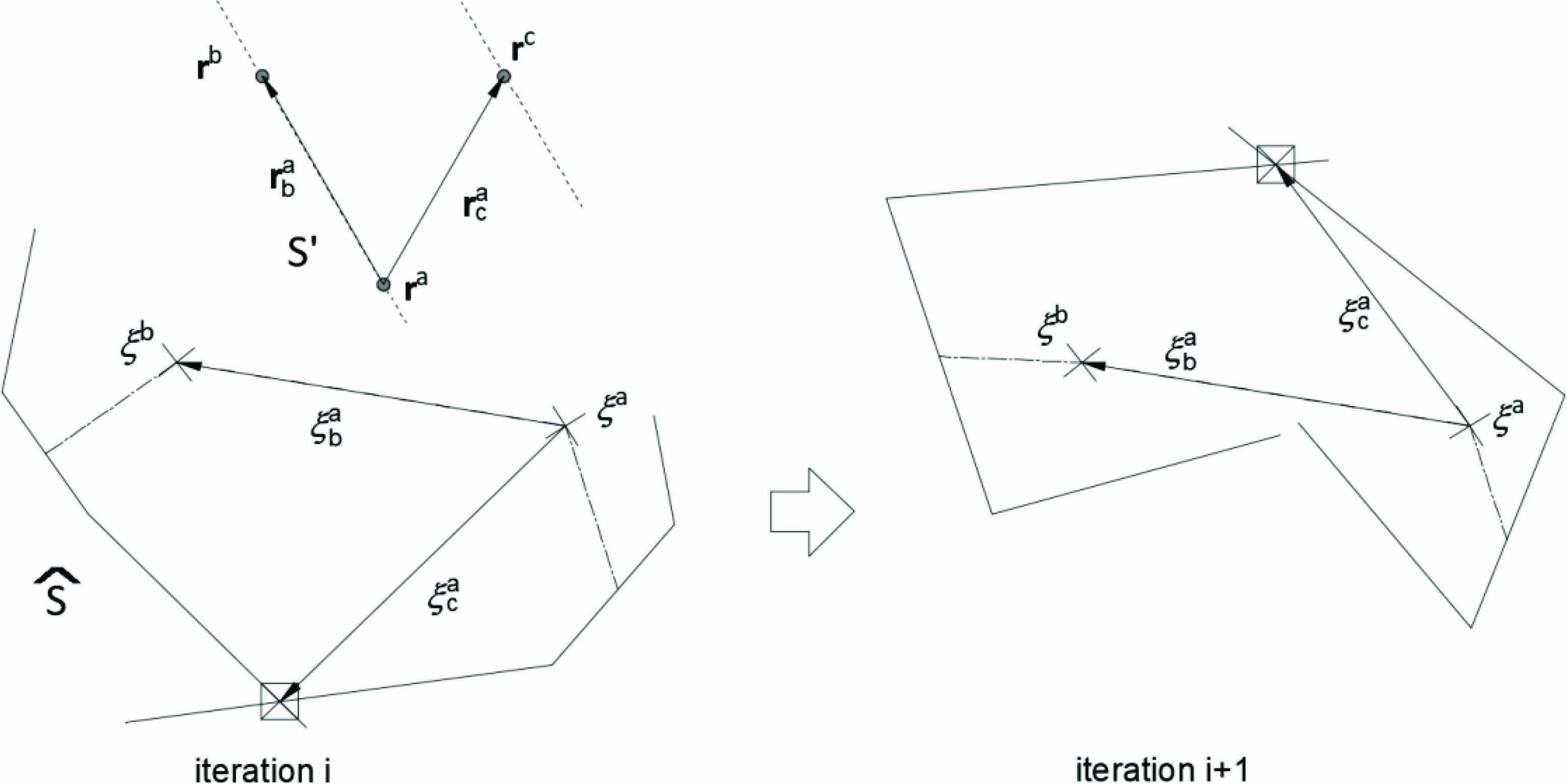
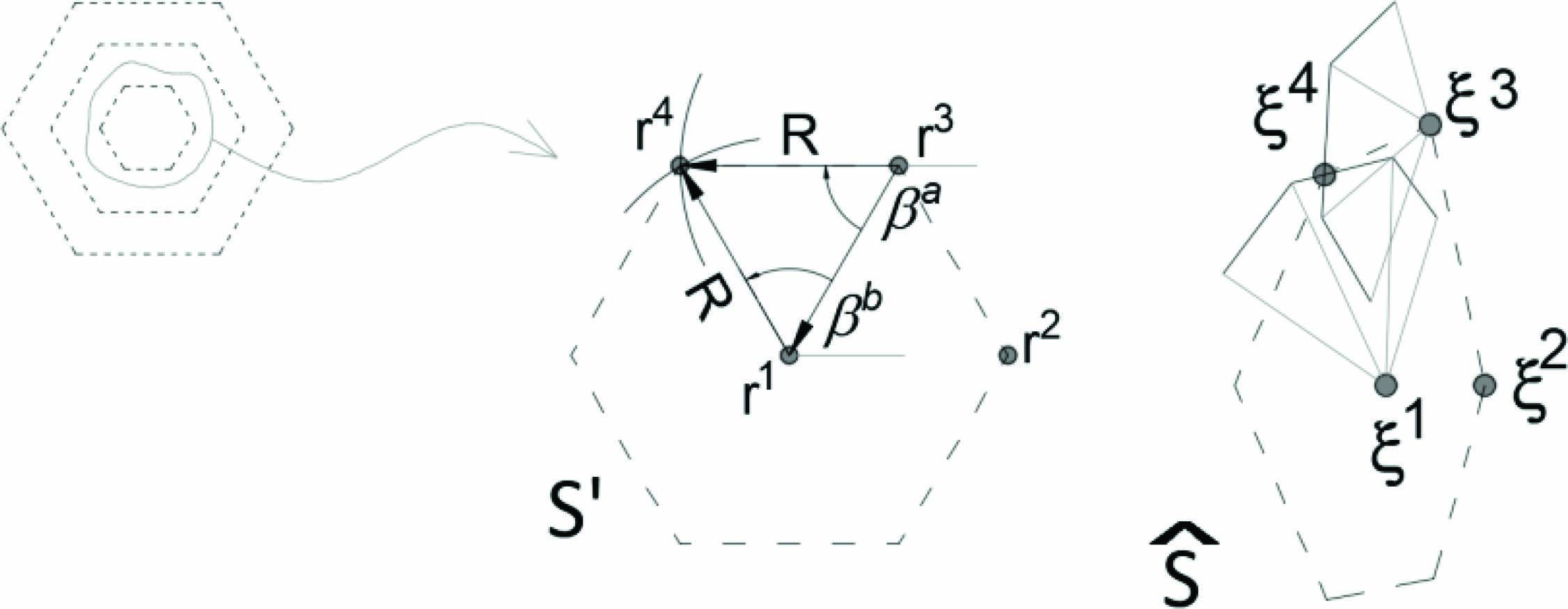
This section explains how to compute the vertexes of the surfaces based on the EPP and AIP algorithms. First, the vertex is arbitrarily placed at the centre of the parameter and pattern spaces, i.e. ${𝝃}^1=(0.5,0.5)$ and ${𝒓}^1=(0,0)$. Second, the vertex is computed by EPP with target distance $R$, orientation $\theta =0$ and initial location ${𝝃}^1$. The rest of the first hexagon vertexes (${𝝃}^3$ to ${𝝃}^7$) are computed by the algorithm AIP from the previous vertex and ${𝝃}^1$, both with radius equal to $R$. Initial trial angles for AIP are ${\beta }^a=-60$ and ${\beta }^b=+60$. Figure 27 illustrates the fourth vertex calculation in the pattern space, showing only the final iteration for clarity.

Figure 27 Fourth vertex computation.

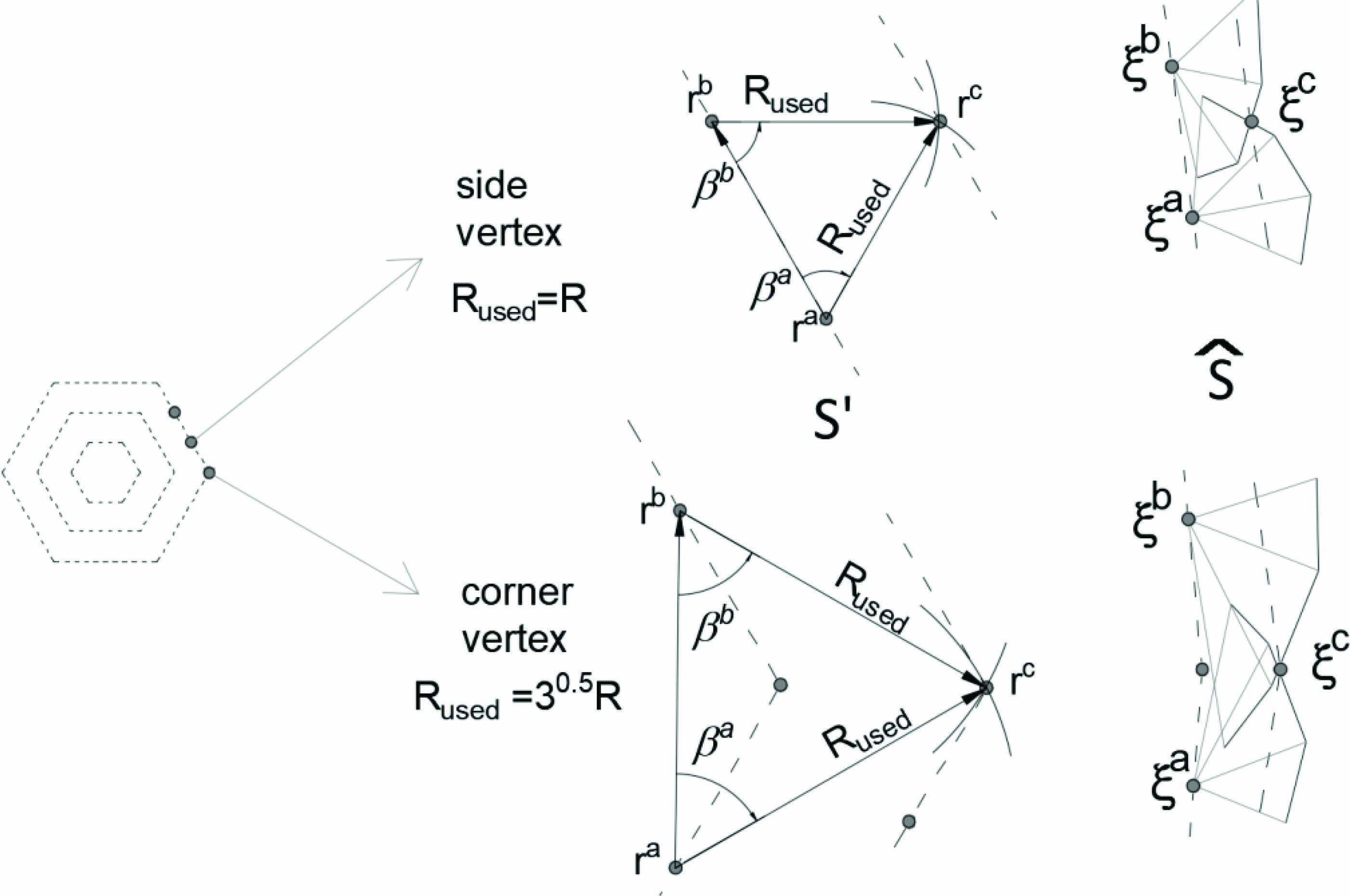
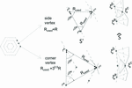
Figure 28 Vertex computation for some contours in the pattern and parameter spaces for side and corner vertexes. Only the final iteration arcs are depicted here for clarity.

The remaining vertexes are computed alongside the creation of the hexagons during their propagating motion in the form of a 2D hexagonal wave. Within one hexagon, each vertex is computed using two vertexes from previous hexagons as centre points for the intersection of the arcs (AIP). This pair, called base vertexes, is selected according to the current vertex position: side or corner (see Figure 28). The base vertexes for the former are the closest of the previous hexagon’s side. The base vertexes for the latter are at both sides of the previous corner. If we call a and b to be the base vertexes and c to be the current vertex, the inputs required for AIP are described in Table 2 for each type of vertex.

Table 2 Inputs used for the intersection of arcs (AIP) to find each type of vertex

Current vertex location	Initial trial angles ${\beta }_a$ and ${\beta }_b$	radius
Side	$-$60 and 60	$R$
corner	$-$60 and 60	$\sqrt{3}R$

Not all the vertexes are computed: one vertex is computed if and only if at least one of its base vertexes lies inside the surface parameter limits. This rule avoids the computation of most of the vertexes that do not lie in the surface, reducing the computational cost considerably. Therefore, the unique hexagonal front that propagates from the central point will be cut and divided into two or more fronts by the surface boundaries during the propagation process, but its divergence is still a possibility. The propagation of contours ends at the hexagon that has all its vertexes non-computed, i.e. all the base vertexes, from previous hexagons, lie outside the surface parameter limits.

Figure 29 Pattern space representation of neighbour vertexes of 22 (side vertex) and 32 (corner vertex). First and second perimeters are indicated in solid line.

One of the base vertexes might be outside the limits in the parameter domain. That vertex involves computations beyond the limits of the surface and this is why the perimeter and corner elements of a dS-mesh are necessary (recall Section 5.1).

5.5 Recovering of Non-Computed Base Vertexes

The procedure described in Section 5.4 might lead to a vertex c with one base vertex non-computed. Let us call a and b to the computed and non-computed base vertexes respectively. If vertex c is to be calculated (we assume a inside surface limits) the base vertex b needs to be estimated. Two carry out this ‘rescue’ of vertex b we need first to identify its neighbours.

The vertexes that surround the b vertex in its first and second perimeters are localized using their relationship in the pattern space (see Figure 29). The relevant information required from these neighbour vertexes are their references, pattern distances and angles measured from vertex $b$. Two of them are then selected, giving priority to the first perimeter and to the pair that form 60 or 120 degrees with each other. The calculation of the b vertex is done by using AIP and the selected neighbour vertexes.

6 Triangulation

This section details the surface triangulation. Section 6.1 explains the calculation of edge vertexes in the pattern space. Section 6.2 gives the criteria to detect non-valid surface vertexes for the triangulation. Section 6.3 shows the triangulation itself and Section 6.4 details the improvement achieved at the edges.

The surface vertexes computed so far may be classified as follows. Let us define $\Delta x_{th}$ as a pre-established threshold distance in the physical space, which is measured from the surface edges (in this work $\Delta x_{th}=R/3$), then:

– SI-vertex: is a surface vertex which lies inside the parameter limits of the surface and is located further away of more than $\Delta x_{th}$ from the edges of the surface.

– SE-vertex: is a surface vertex inside the parameter limits of the surface and lies within a distance lower than $\Delta x_{th}$ when measured from the edges of the surface.

– SO-vertex: is a surface vertex which lies outside of the surface parameter limits.

6.1 Estimation of Edge Vertexes in the Pattern Space

The edge vertexes’ coordinates in the pattern space are part of the final triangulation procedure and, furthermore, they form the constraint that determines which triangles are inside or outside of the computable domain. Since these coordinates are unknown (edge vertexes were computed independently, see Section 4) they need to be estimated.

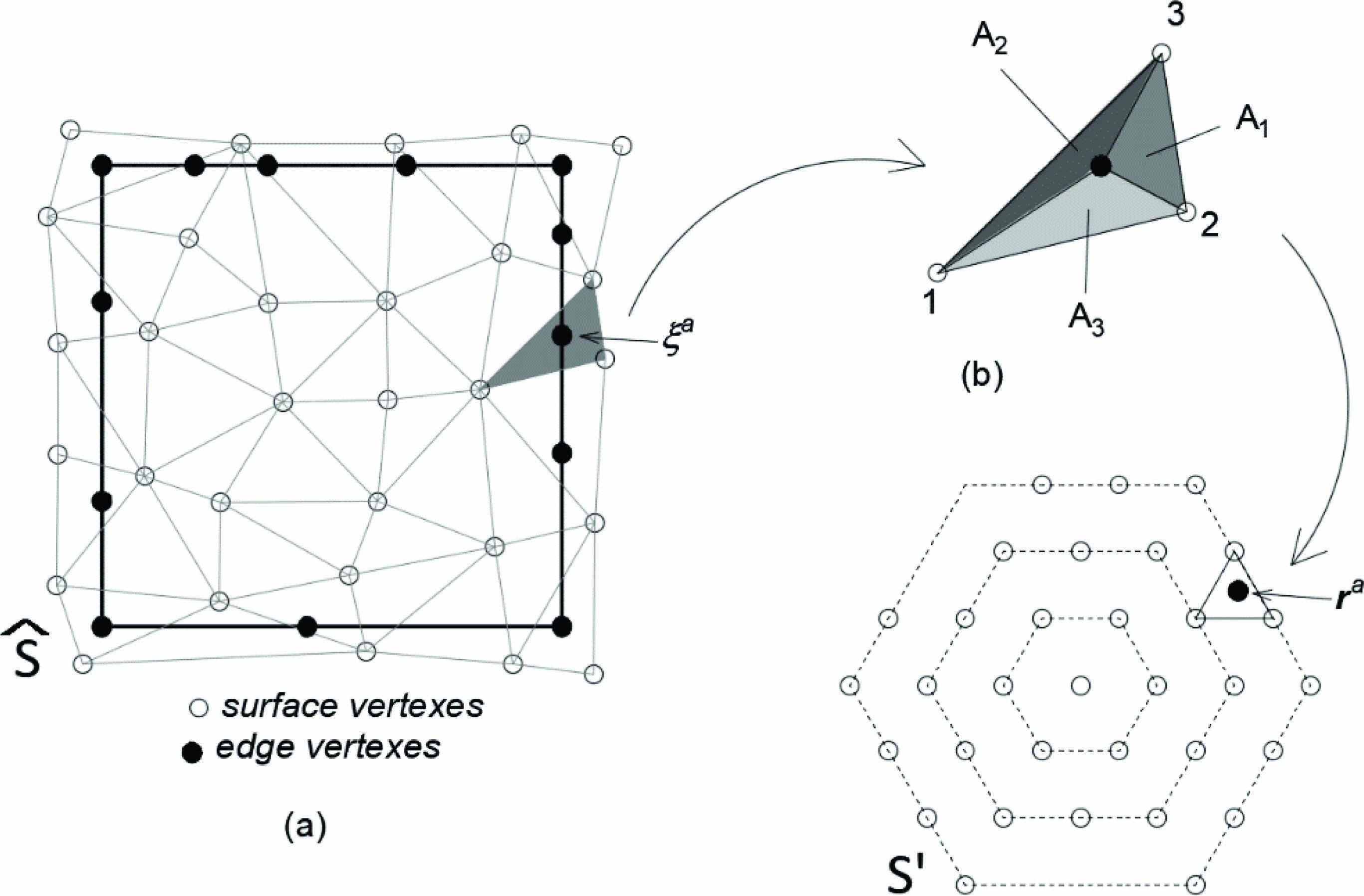
We construct a triangulation with all surface vertexes (SO, SE and SI-vertexes) in the parameter space. This triangulation allows the mapping ${ℝ}^2\to {ℝ}^2$ from the surface parameter space to the pattern space. The parameter coordinates for the edge vertexes lie within this triangular net, therefore their pattern coordinates may be calculated by the following mapping:

$${𝒓}^a=\sum _{i=1}^3{N}_i{𝒓}^i$$

(19)

Where shape functions $N_i$ are the area coordinates, as defined in Equation (20), where $A_{total}$ is the area of the triangle and $A_i$ are the sub-areas attached to each node of the triangle. In Figure 30, one example for the computation of the pattern coordinates for vertex $a$ is illustrated.

$$N_i=\frac{A_i}{A_{total}}$$

(20)

Figure 30 Triangulation of all vertexes in the parameter space (a) and calculation of the pattern coordinates of the edge vertex $a$ (b).

The triangulation explained in this section is not the final aim chased by the QIT procedure but it is a temporary triangulation that permits the estimation of the pattern coordinates of edge vertexes with some degree of accuracy.

6.2 Removal of Non-Valid Surface Vertexes

Only SI-vertexes are considered in the triangulation (valid vertexes). Meanwhile SO and SE-vertexes are non-valid. SO-vertexes are detected because they are located on the outside of the surface limits. SE-vertexes are closer than $\Delta x_{th}$ to the edges of the surface. To measure the distance from one surface vertex to the edges, the closest pair of edge vertexes needs to be found. Then the distance from the vertex to the segment between both edge vertexes is computed in the physical space.

6.3 Delaunay Triangulation in the Pattern Space

Triangulation is done in the pattern space mainly for two reasons:

– It will be quasi-isotropic, given the vertexes arrangement of this space.

– It is a 2D plane space that facilitates the entire process.

The resultant triangulation in the physical space will inherit the same features of the triangulation on the pattern space since the location of its vertexes follows the same scheme.

Valid surface and edge vertexes obtained in previous steps are used in this section for the Delaunay triangulation. Edge vertexes impose constraints to the triangulation: they form the perimeter of the domain (see Figure 31).

Figure 31 All vertexes and resultant triangulation with valid vertexes in the pattern space.

6.4 Edge Strip Triangles Amendment

Let us call edge triangles strip to triangles that have at least one edge vertex. As the pattern coordinates of edge vertexes were already estimated (Section 6.2) they might not yield the highest quality triangulation in the physical space along this strip.

A localized improvement through the edge triangles strip is needed to reduce their distortion. Since not all the triangles are to check but only the edge strip ones, the process is computationally cheap. Triangles are selected in pairs, forming one quadrilateral, in advancing sequence along the four different edges separately. In each quadrilateral, both diagonals are measured in the physical space and the shortest diagonal is selected, which might coincide with the original or might not (the diagonal is then flipped). Quadrilaterals with at least one angle greater than 180${}^{\circ }$ are not checked. Figure 32 illustrates one example for demonstration purposes, where only one edge strip is detailed for clarity.

Figure 32 Edge triangles strip before (a) and after (b) improvement. Quadrilaterals advancing at left edge (c).

7 Numerical Examples

The aim of the two examples presented in this section is to demonstrate the performance of QIT. Geometry and algorithm input details are listed in Appendix D. For both examples, the resultant mesh from the proposed QIT algorithm is compared with the equivalent highest quality triangulation ideally achievable, that we call BIT (acronym for ‘Bounded Isotropic Triangulation’). Details of such triangulation are provided in Appendix C, but here we list the most relevant features:

– All angles are sixty degrees.

– All triangles have the same area: $A_{BIT}=\frac{R^2}{4}tan60$.

– Vertexes valences frequency is the closest possible to the ideal case: two vertexes of valence 2, two with valence 4, a few with valence 3 and the rest with valence 6.

To characterize the triangulation performance, we set intervals for angles, triangle sizes and valences, and count the number of instances in each interval to obtain the frequency, expressed in percentage. The frequencies are plotted and compared against the BIT reference solutions. In addition, the so-called quality index $Q$ described in Equation (21), is computed. This is a numerical indicator in percentage of how close the triangulation is to the BIT reference solution. The ideal value is 100%.

$$Q=25\frac{f_s^a}{100}+25\frac{f_n^a}{100}+25\frac{f_{v3}^a}{f_{v3}^b}+25\frac{f_{v6}^a}{f_{v6}^b}$$

(21)

The inputs for Equation (21) are frequencies, in percentage, for:

$f_s^a$: triangles of QIT, with sizes in the same interval as BIT size ($A_{BIT}$);

$f_n^a$: angles of QIT in the same interval of 60 degrees;

$f_{v3}^a$ and $f_{v3}^b$: vertexes with the valence number equal to 3 for both QIT and BIT;

$f_{v6}^a$ and $f_{v6}^b$: vertexes with the valence number equal to 6 for both QIT and BIT.

Note that the frequencies for the size and angles for the BIT are 100%.

7.1 Single Surface with Severe Distortion in the Parameter Space

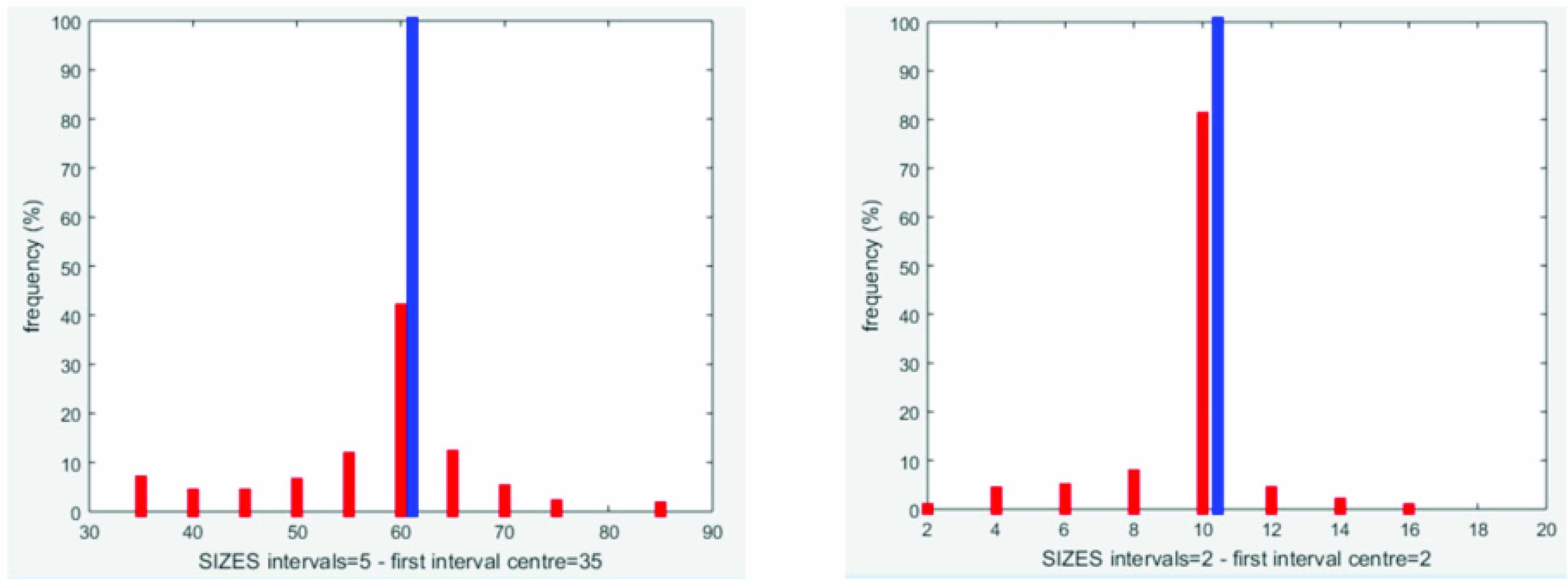
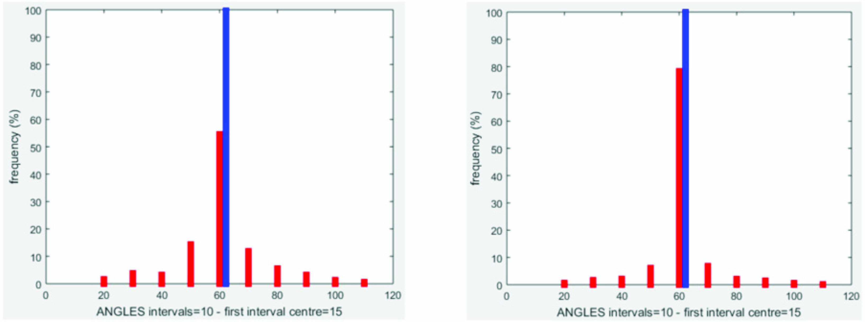
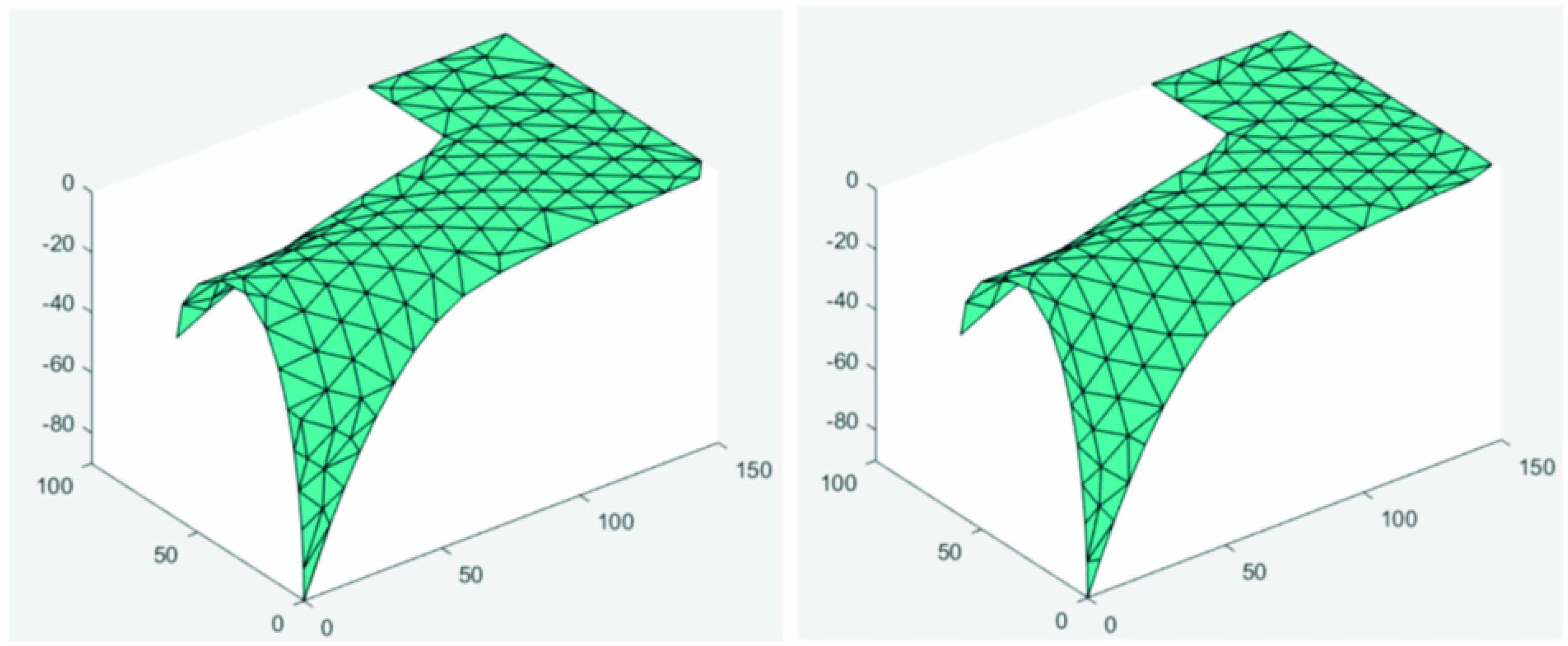
A single surface with abrupt increments in parameter space is meshed with our QIT algorithm. The algorithm was performed for two different sizes: $R=12$ and $R=5$. Derivatives were estimated by spline surface fitting, as described in Appendix B. In spite of the distortion in the parameter space, the resultant triangulations remain mostly isotropic, only some few triangles appear to be distorted due to the presence of edges. The quality factor $Q$ is greater when $R=5$ because the number of triangles affected by the edges is less than in the other case when $R=12$. This indicates that if the edges have a small influence on the overall surface’s domain then the closer to the BIT reference solution is the QIT triangulation and, therefore, it proves that the QIT method brings onto the surface physical space an accurate ‘image’ of the pattern space.

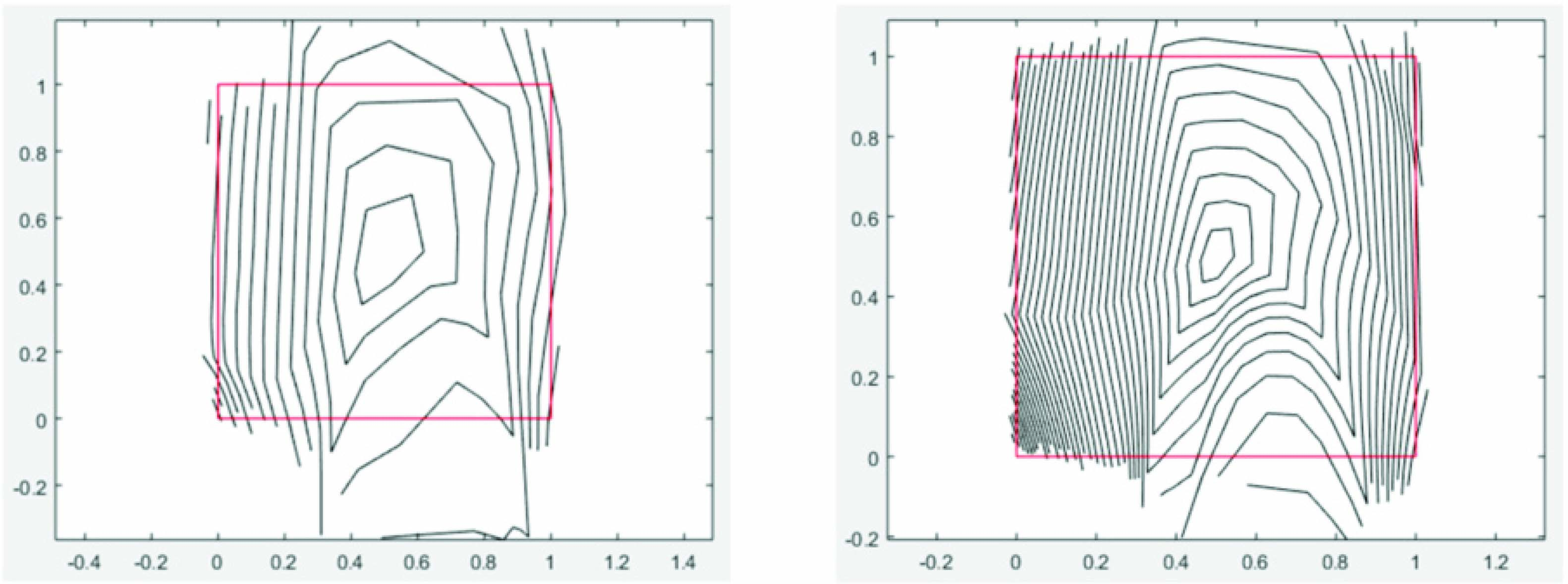
Figure 33 shows the surface in the physical space with the knot spans depicted and one triangulation with vertexes equally spaced in the parameter space to highlight the distortion in the parametrization. Figure 34 illustrates the QIT method with both $R=12$ and $R=5$. Figure 35 shows the propagation of contours in the parameter space, where the divergent nature of the front can be clearly seen, note also some of the contours go further off the surface limits. Figures 36 to 38 show the frequency plots.

Figure 33 Left: surface for triangulation. Right: triangulation with nodes equally spaced in the parameter space.

Figure 34 Resultant QIT triangulation. Left: $R=12$. Right: $R=5$.

Figure 35 Contours propagation in the parameter space, red lines are the surface limits. Left: $R=12$. Right: $R=5$.

Figure 36 Frequency plots for triangle sizes. Red represents the QIT while blue represents the BIT. Left: $R=12$. Right: $R=5$.

Figure 37 Frequency plots for angles. Red represents the QIT while blue represents the BIT. Left: $R=12$. Right: $R=5$.

Figure 38 Frequency plots for valences. Red represents the QIT while blue represents the BIT. Left: $R=12$. Right: $R=5$.

The quality index (Q) is computed below for both cases. Note how the quality raises from 62 to 80% when the target distance decreases from 12 to 5, i.e. if a finer mesh is used then it gets closer to the ideal BIT.

$Q$	$=25⁤{\displaystyle \frac{41}{100}}+25⁤{\displaystyle \frac{55}{100}}+25⁤{\displaystyle \frac{24}{33}}+25⁤{\displaystyle \frac{51}{65}}=62\%$
$Q$	$=25⁤{\displaystyle \frac{78}{100}}+25⁤{\displaystyle \frac{80}{100}}+25⁤{\displaystyle \frac{12}{18}}+25⁤{\displaystyle \frac{75}{81}}=80\%$

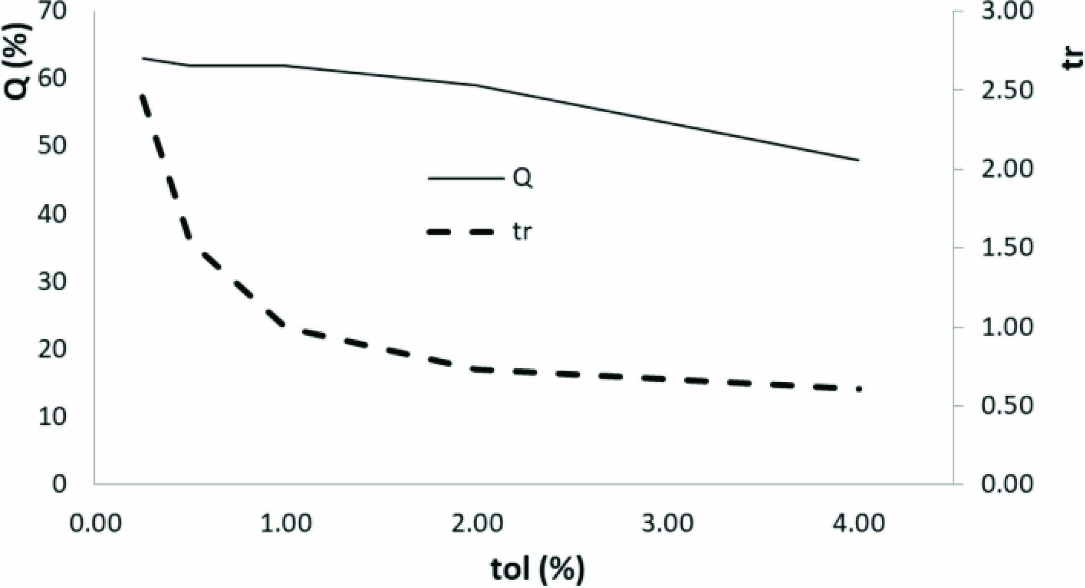
To illustrate the influence of the tolerance in the computational cost, Figure 39 is used. It includes the plot for the relative computational time (tr) for edge vertex tolerances of 0.25, 0.50, 1.0, 2.0 and 4.0% (vertical axis on the right-hand side of the plot). The surface vertex tolerances are 4 times larger, e.g. 2.0% for the tolerance for edge vertexes, the tolerance for surface vertexes is 8.0%. The triangle size used was $R=12$. That relative computational time is referred to the tolerance of 1.0% for edges. It also includes the quality index (Q), which is plotted in the vertical axis on the left-hand side of the plot. It can be clearly seen that it decreases as the tolerance becomes larger, as expected.

Figure 39 Relative computational time (tr) and quality index (Q) versus tolerances.

The quality improvement with the tolerance restriction can also be seen in Figure 40, where the resultant meshes are depicted for tolerances of 4.0 and 0.25%.

Figure 40 Triangulation for tolerances of 4.0 % (left) and 0.25% (right).

7.2 Three Contiguous Surfaces

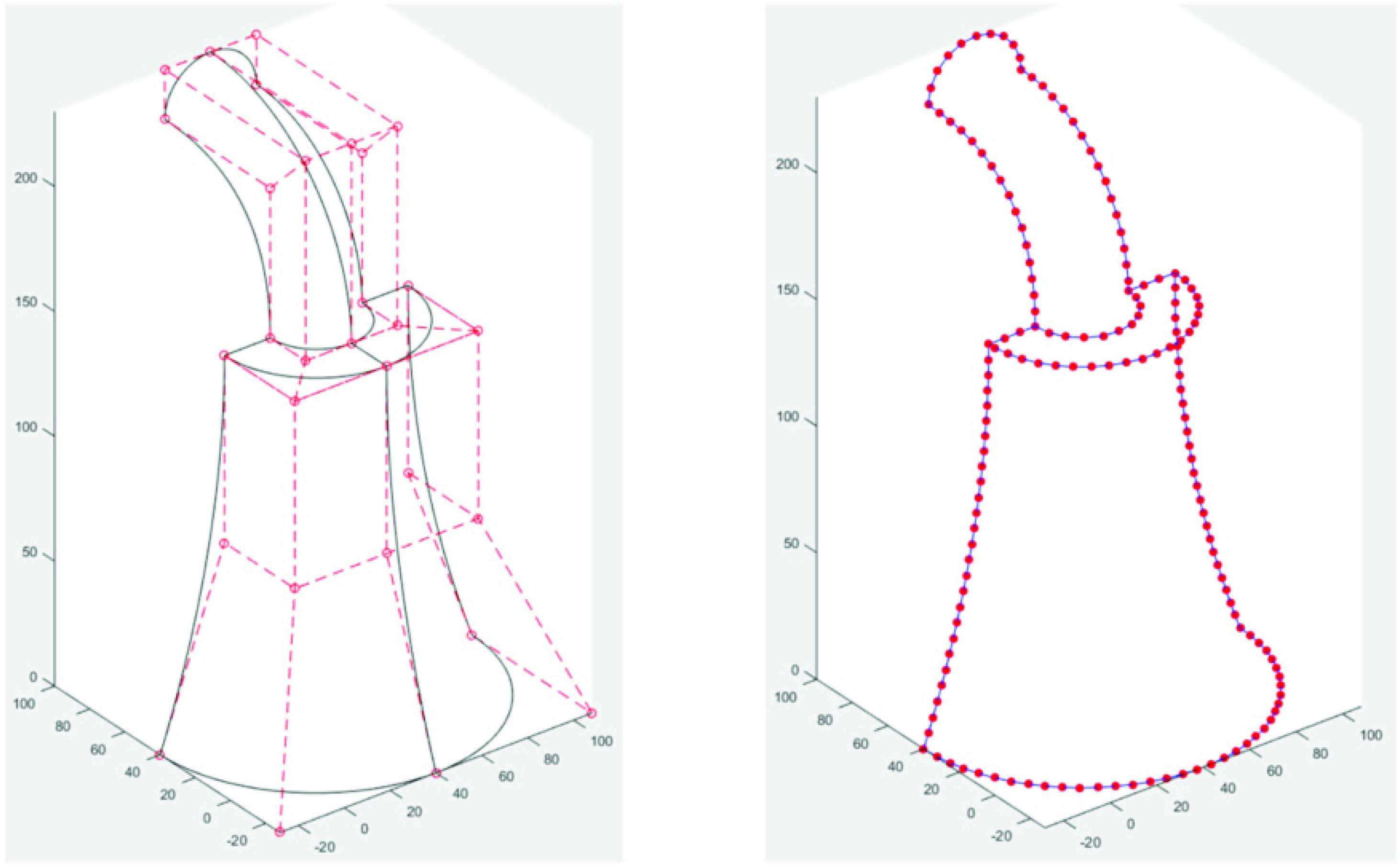
Figure 41 Left: surfaces for triangulation. Right: edge vertexes resultant from the QIT algorithm.

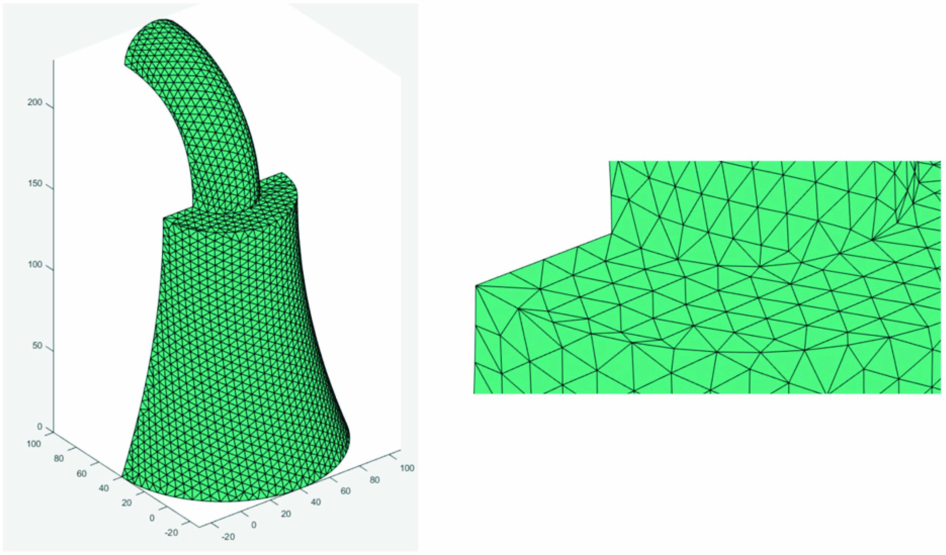
This example shows how three contiguous surfaces are conformal triangulated using the QIT algorithm, i.e. their shared edges have the same curve discretization. The target distance used was $R=5$. Figure 41 gives the surfaces in the physical space with knot spans and control points (left) and the computed edge vertexes (right). Figure 42 shows the final result after triangulation (left), where the general isotropy and uniformity of the triangulation can be clearly observed. On the right side of that figure, the edge shared by contiguous surfaces is detailed, where conformal meshes can be observed. Finally, Figure 43 provides the frequency plots showing again the tendency of the QIT algorithm to achieve mesh isotropy close to the perfect solution delivered by BIT. The quality index for this case is 73 %, as calculated below.

$$Q=25⁤\frac{54}{100}+25⁤\frac{77}{100}+25⁤\frac{9}{13}+25⁤\frac{80}{86}=73\%$$

Figure 42 Left: resultant mesh from the QIT algorithm. Right: detail for the merging of the mesh for different surfaces.

Figure 43 Frequencies of sizes, angles and valences. Red represents our QIT and blue BIT.

8 Conclusions and Future Work

A new procedure for triangulating NURBS surfaces is presented in this work. It provides a quasi-isotropic triangular mesh at once, with no preliminary tessellation, based on a divergent advancing front technique that avoids front collisions. Each new vertex position is calculated using trapezoidal numerical integration, which provides simplicity and therefore efficiency. The error committed in this approximation is controlled by previous discretization of the parameter space. When there is more than one surface involved, their meshes are conformal at the shared curve because vertexes of such curve are computed once and applied for both surfaces. Derivatives are required repeatedly for this algorithm. In order to improve the efficiency, alternatives to the analytical calculation of these derivatives are proposed in Appendix B.

The examples proposed demonstrated that the method delivers high quality triangulations that tend to be isotropic, regardless of the shape or parametrization used. Potential extensions or improvements of the method are listed below:

– This procedure applies to non-trimmed surfaces. Application to trimmed surfaces is still pending.

– Triangulations obtained by the algorithm presented here might be the initial stage for further refinements at certain zones such as high curvature areas or where analysis results (e.g. strains) are expected to present sudden variations.

Acknowledgments

The authors gratefully acknowledge the Department of Engineering Design and Mathematics of the University of the West of England that partially founded this research. They also acknowledge to Dr. Arnaud Marmier, senior lecturer at the same university, for his comments on this work.

Appendixes

Appendix A: Derivatives of a Function that is as Norm of First Derivative of Another Function

Let $f(u)$ be a function defined as the norm of first derivative of another function $𝒈(u):{ℝ}^1\to {ℝ}^d$. For the sake of clarity we remove the free variable from the notation, then $f(u)$ is expressed as $f$, $𝒈(u)$ as $𝒈$ and so on.

$$𝒈\mathbf{=}{g}_i\forall i=1tod$$

(A.1)

$$f=\parallel 𝒈{}^{\mathbf{\prime }}\parallel ={\left(\sum _{i=1}^{d}g_i^{\prime }{}^2\right)}^{1/2}$$

(A.2)

First derivative of $f$ is computed by simple differentiation of (A.2), that yields (A.3).

$$f^{\prime }=\frac{{\sum }_{i=1}^d\left(g_i^{\prime }{g}_i^{\prime \prime }\right)}{f}$$

(A.3)

Applying differentiation again to (A.3) we obtain the second derivative of $f$, written in (A.4).

$$f^{\prime \prime }=\frac{{\sum }_{i=1}^d\left(g_i^{\prime \prime }{g}_i^{\prime \prime }+g_i^{\prime }{g}_i^{\prime \prime \prime }\right)f-{\sum }_{i=1}^d\left(g_i^{\prime }{g}_i^{\prime \prime }\right)f^{\prime }}{f^2}$$

(A.4)

For NURBS surfaces $𝑺(\xi ,\eta )$ the directional derivatives are functions of main derivatives ($𝑺{,}_{\xi }$ and $𝑺{,}_{\lambda }$) and are not trivial. First directional derivative $g_i^{\prime }=𝑺{,}_{\lambda }$ is (A.5).

$$𝑺{,}_{\lambda }=𝑺{,}_{\xi }cos\theta +𝑺{,}_{\eta }sin\theta$$

(A.5)

Second $g_i^{\prime \prime }=𝑺{,}_{\lambda \lambda }$ and third $g_i^{\prime \prime \prime }=𝑺{,}_{\lambda \lambda \lambda }$ directional derivatives are explained here. Let $𝝂$ be a vector with orientation $\theta$ and $\parallel 𝝂\parallel =1$, i.e. ${\nu }_1=\cos \theta$ and ${\nu }_2=\sin \theta$. Let $S(𝝃)$ be a function such that $𝒈(u):{ℝ}^2\to {ℝ}^1$ with $𝝃={(\xi ,\eta )}^T$. Derivatives w.r.t. $\xi$ and $\eta$ at location ${𝝃}_0$ may be calculated as expressions (A.6) and (A.7).

$$S{,}_{\xi }=\underset{h\to 0}{lim}\frac{S({𝝃}_0+(h,0))-S({𝝃}_0)}{h}=\underset{h\to 0}{lim}\frac{S({\xi }_0+h,{\eta }_0)-S({\xi }_0,{\eta }_0)}{h}$$

(A.6)

$$S{,}_{\eta }=\underset{h\to 0}{lim}\frac{S({𝝃}_0+(0,h))-S({𝝃}_0)}{h}=\underset{h\to 0}{lim}\frac{S({\xi }_0,{\eta }_0+h)-S({\xi }_0,{\eta }_0)}{h}$$

(A.7)

Directional first derivative of $S$ with $\theta$ orientation at location ${𝝃}_0$ is given by Equation (A.8), which is equivalent to (A.9).

$$S{,}_v=\underset{h\to 0}{lim}\frac{S\left({𝝃}_0+h𝒗\right)-S({𝝃}_0)}{h}=\underset{h\to 0}{lim}\frac{S({\xi }_0+h{v}_1,{\eta }_0+h{v}_2)-S({\xi }_0,{\eta }_0)}{h}$$

(A.8)

$$S{,}_v=\mathbf{\nabla }𝑺\cdot 𝝂={\left\{\begin{array}{c}\hfill S{,}_{\xi }\hfill \\ \hfill S{,}_{\eta }\hfill \end{array}\right\}}^T\left\{\begin{array}{c}\hfill {\nu }_1\hfill \\ \hfill {\nu }_2\hfill \end{array}\right\}$$

(A.9)

Directional second derivative is obtained as follows:

$$S{,}_{\nu \nu }=\underset{h\to 0}{lim}\frac{\left({lim}_{h\to 0}\frac{S\left({𝝃}_0+h𝝂+h𝝂\right)-S({𝝃}_0+h𝝂)}{h}\right)-\left({lim}_{h\to 0}\frac{S\left({𝝃}_0+h𝝂\right)-S({𝝃}_0)}{h}\right)}{h}$$

(A.10)

$$S{,}_{\nu \nu }=\underset{h\to 0}{lim}\frac{S\left({𝝃}_0+2h𝝂\right)-2S\left({𝝃}_0+h𝝂\right)+S({𝝃}_0)}{h^2}$$

(A.11)

Developing Equation (A.11) and grouping terms we arrive to the bilinear form (A.12), which is equivalent to (13).

$$S{,}_{\nu \nu }={𝒗}^T𝑯𝒗=\left\{\begin{array}{cc}\hfill {\nu }_1\hfill & \hfill {\nu }_2\hfill \end{array}\right\}\left[\begin{array}{cc}\hfill S{,}_{\xi \xi }\hfill & \hfill S{,}_{\xi \eta }\hfill \\ \hfill S{,}_{\xi \eta }\hfill & \hfill S{,}_{\eta \eta }\hfill \end{array}\right]\left\{\begin{array}{c}\hfill v_1\hfill \\ \hfill v_2\hfill \end{array}\right\}$$

(A.12)

$$S{,}_{\nu \nu }={\nu }_i{\nu }_{j}S{,}_{ij}\forall i,j=1,2$$

(A.13)

In (A.13), sub-index of $S{,}_{ij}$ indicates derivatives w.r.t. $\xi$ (sub-index $=$1) or $\eta$ (sub-index=2). Same procedure for third directional derivative yields Equation (A.14):

$$S{,}_{\nu \nu \nu }=\underset{h\to 0}{lim}\frac{S({𝝃}_0+3h𝝂)-3S({𝝃}_0+2h𝝂)+3S({𝝃}_0+h𝒗)+S({𝝃}_0)}{h^3}$$

(A.14)

Developing (A.14) and grouping terms, the third directional derivative can be expressed as (B.15).

$$S{,}_{\nu \nu \nu }={\nu }_i{\nu }_j{v}_{k}S{,}_{ijk}\forall i,j=1,2$$

(A.15)

Where sub-index of $S{,}_{ijk}$ indicates derivatives w.r.t. $\xi$ (sub-index $=$1) or $\eta$ (sub-index=2).

So far, third directional derivatives expression (A.9), (A.13) and (A.15) are deducted for functions $S:{ℝ}^2\to {ℝ}^1$. Application for function $𝑺:{ℝ}^2\to {ℝ}^d$ is direct. Each of the $d$ components of the directional derivative can be calculated separately by Equations (A.9), (A.13) and (A.15). For example for $d=3$ ($𝒙=x,y,z$) third directional derivative has three components as per Equation (A.16).

$S^x{,}_{\nu \nu \nu }$	$=$	${\nu }_i{\nu }_j{\nu }_k{S}^x{,}_{ijk}\forall i,j=1,2$
$S^y{,}_{\nu \nu \nu }$	$=$	${\nu }_i{\nu }_j{\nu }_k{S}^y{,}_{ijk}\forall i,j=1,2$	(A.16)
$S^z{,}_{\nu \nu \nu }$	$=$	${\nu }_i{\nu }_j{\nu }_k{S}^z{,}_{ijk}\forall i,j=1,2$

Appendix B: Surface Derivatives Estimation

Analytical calculation of NURBS derivatives is computationally expensive. To increase the algorithm speed we propose two alternatives. In both cases analytical derivatives are calculated previously at certain locations (sample points) and then a surface is fitted to them. The first presented method fits spline surfaces to those sample points. The second method uses the dS-mesh nodes as sample points to linearly interpolate between them. We recall that $\theta$-directional derivative is computed as per Equation (B.1).

$$𝑺{,}_{\lambda }=𝑺{,}_{\xi }cos\theta +𝑺{,}_{\eta }sin\theta$$

(B.1)

B.1 Derivatives Computed from Fitted B-spline Surfaces

B.1.1 Basic Definitions

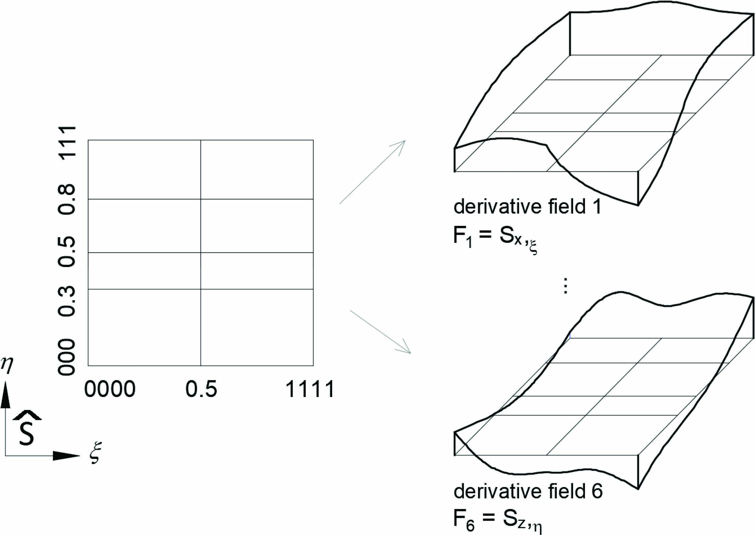
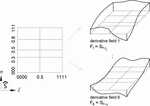
Let $𝑭(\xi ,\eta ):{ℝ}^2\to {ℝ}^6$ be a function that store the NURBS surface $𝑺(\xi ,\eta )$ derivatives fields, i.e. $S_j{,}_{\beta }$ with $j=1,2,3$ that corresponds to $x,y,z$ components; and $\beta =1,2$ for derivatives w.r.t. $\xi$ and $\eta$. The domain of $𝑭$ is the parameter space of $𝑺$. The $i$th component of $𝑭$ corresponds to $jx\beta$. Figure B.1 shows two examples.

Figure B.1 Derivatives fields of NURBS surface showing the first and last derivatives components.

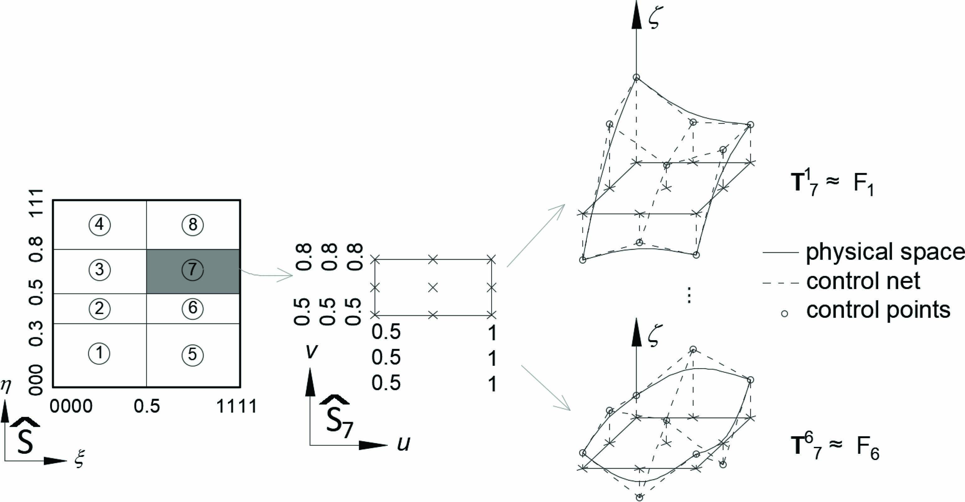
We define in each knot span of $𝑺$ a set of six spline surfaces to approximate the six components of $𝑭$. Spline¹ surface $𝑻^i{}_k:{ℝ}^2\to {ℝ}^3$ is to be fitted to the $(\beta xj)$th derivative component within the $k$th knot span of $𝑺$. We will refer to each of those sets of six spline surfaces as k-set.

$𝑻^i{}_k$ has the parameter space ${\widehat{\mathrm{S}}}_k$ with components $(u,v)$ and maps onto ${ℝ}^3$, with two first components, called plan coordinates, equal to $(u,v)$ and the third component, called height ($\zeta$), with the $F_{𝒊}$ derivative estimation, (see Figure B.2).

Figure B.2 k-set for the seventh span of the NURBS surface (first and last components are shown).

Features of each k-set are listed below:

– Parameter space domain coincides with the correspondent $𝑺$ knot span domain: ${\widehat{\mathrm{S}}}_k=({\xi }_{k1},{\xi }_{k2})\otimes ({\eta }_{k1},{\eta }_{k2})$, where ${\xi }_{k1},{\xi }_{k2},{\eta }_{k1}$ and ${\eta }_{k2}$ are the kth knot span limits.

– Control points plan coordinates coincide with their parameter coordinates $(u,v)$, therefore one parameter location for $𝑻^i{}_k$ coincides with its physical plan coordinates and with the parameter coordinates of $𝑺$.

– Control points are equally spaced on plan in each direction, i.e. plan coordinates form a regular net on ${\widehat{\mathrm{S}}}_k$.

– The six splines of the k-set share the same plan coordinates, hence they share parametrization.

– The six splines of the k-set share basis functions, i.e. they use the same knot spans, degrees and number of control points.

– Control points heights are to be fitted to the correspondent derivatives field, e.g. $𝑻^3{}_k$ fits to $F_3=S_{1,3}=S_{z,\xi }$.

There is one k-set defined separately for each knot span of $𝑺$ in order to guarantee that those splines are fitted to a smooth field avoiding any potential $C^0$ transition between knot spans. The fitted splines in this work are quadratic. Previously to fit $𝑻^i{}_k$ splines to derivatives fields $S_{j,\beta }$, we need to define the number of control points in each direction, which is driven by the error estimation as shown in Section B.2.2.

B.1.2 Number of Control Points

Explanations in this section are given for one k-set and one derivative field $F_i$. Sub-index on $F$ is removed for clarity. The number of control points is driven by the estimation of error. Absolute error is given by equation (B.2), that is deducted in Section B.2.5.

$E$	$\le$	$|{\displaystyle \frac{1}{3!}}(F^{𝜶}{,}_{\xi \xi \xi }\mathrm{\Delta }\xi _r{}^3+3F^{𝜶}{,}_{\xi \xi \eta }\mathrm{\Delta }\xi _r{}^2\mathrm{\Delta }{\eta }_r+3F^{𝜶}{,}_{\eta \eta \xi }\mathrm{\Delta }\eta _r{}^2\mathrm{\Delta }{\xi }_r$	(B.2)
		$+F^{𝜶}{,}_{\eta \eta \eta }\mathrm{\Delta }\eta _r{}^3\left)\right|$

Where $\mathrm{\Delta }{\xi }_r$ and $\mathrm{\Delta }{\eta }_r$ are the representative increments (see section B.2.5, Equation B.28) and derivatives are at location $𝜶=({\xi }_{\alpha },{\eta }_{\alpha })$ that belongs to the knot span sub-domain ${\widehat{\mathrm{S}}}_k$ and maximises the error. Relative error in percentage is obtained as equation (B.3), being $\overline{F}$ the root mean square over the whole knot span (B.4) that might be estimated by Gauss quadrature.

$$E_r=100E/\overline{F}$$

(B.3)

$$\overline{F}=\sqrt{\frac{1}{Are{a}_{{\widehat{\mathrm{S}}}_k}}{\int }_{{\widehat{\mathrm{S}}}_k}F𝑑{\widehat{\mathrm{S}}}_k}$$

(B.4)

$E_r$ in the derivative estimation is to be equal or less than the prescribed tolerance. This condition will determinate the number of control points for the k-set following next steps:

– Initial number of control points corresponds to $𝑻^i{}_k$ spline with a single knot span, since $𝑻^i{}_k$ is quadratic, initial number of control points is three in each direction. Therefore initial representative plan increments are $\mathrm{\Delta }\xi ^0{}_r=0.72({\xi }_{k2}-{\xi }_{k1})/2$ and $\mathrm{\Delta }\eta ^0{}_r=0.72({\eta }_{k2}-{\eta }_{k1})/2$, where ${\xi }_{k1},{\xi }_{k2},{\eta }_{k1}$ and ${\eta }_{k2}$ are the knot span limits.

– Third derivatives are needed, but $𝜶$ location is unknown, then we calculate exact derivatives values $F{,}_{\xi \xi \xi },F{,}_{\xi \xi \eta },F{,}_{\eta \eta \xi }$ and $F{,}_{\eta \eta \eta }$ at locations of a net of $s\times s$ equally spaced (in this work $s=3$).

– $E_r$ is computed with equations (B.2), (B.3) and (B.4) for each of these $s\times s$ points using the initial representative increments $\mathrm{\Delta }\xi ^0{}_r$ and $\mathrm{\Delta }\eta ^0{}_r$. We consider only the highest value among the $s\times s$ errors.

– The ratio $d=E_r/tolerance$ is calculated.

– To reduce our error by a $d$ factor, we can only reduce the representative increments as shown in Equation (B.5).

$E/d$	$\le$	$|{\displaystyle \frac{1}{3!}}(F^{𝜶}{,}_{\xi \xi \xi }\Delta \xi _r{}^3/d+3F^{𝜶}{,}_{\xi \xi \eta }\Delta \xi _r{}^2\Delta {\eta }_r/d$	(B.5)
		$+3F^{𝜶}{,}_{\eta \eta \xi }\Delta \eta _r{}^2\Delta {\xi }_r/d+F^{𝜶}{,}_{\eta \eta \eta }\Delta \eta _r{}^3/d\left)\right|$

– We use first and last summands of (B.5) to estimate updated increments in each direction to reduce the error below tolerance, as shown in Equations (B.6) and (B.7).

$$\mathrm{\Delta }{\xi }_r={\left(\frac{\mathrm{\Delta }\xi _r^0{}^3}{d}\right)}^{1/3}=\frac{0.72({\xi }_{k2}-{\xi }_{k1})/2}{d^{1/3}}$$

(B.6)

$$\mathrm{\Delta }{\eta }_r={\left(\frac{\mathrm{\Delta }\eta _r^0{}^3}{d}\right)}^{1/3}=\frac{0.72({\eta }_{k2}-{\eta }_{k1})/2}{d^{1/3}}$$

(B.7)

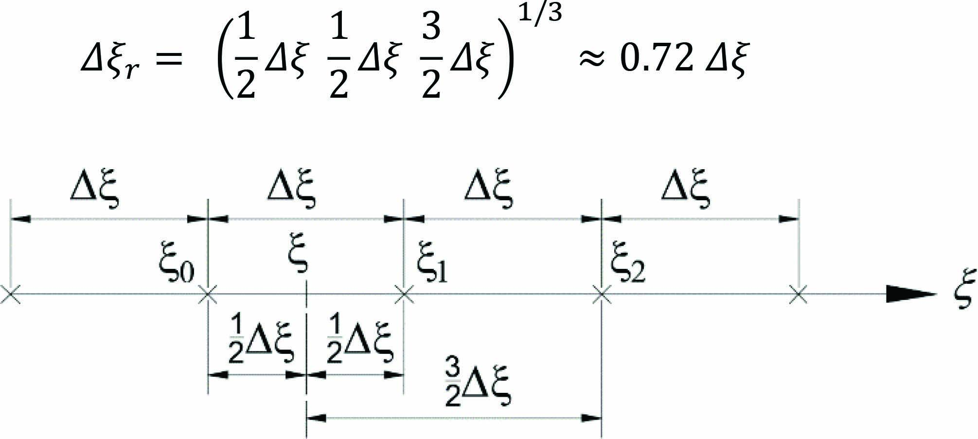
– With these representative increments ($\Delta {\xi }_r$, $\Delta {\eta }_r$) the actual increments ($\Delta \xi$, $\Delta \eta$) are obtained dividing by 0.72 and then the number of control points in each direction is calculated as (B.8) and (B.9).

$$n=max[3,round\left(\frac{\left({\xi }_{k2}-{\xi }_{k1}\right)}{\Delta {\xi }_r/0.72}\right)]$$

(B.8)

$$m=max[3,round\left(\frac{\left({\eta }_{k2}-{\eta }_{k1}\right)}{\Delta {\eta }_r/0.72}\right)]$$

(B.9)

The number of control points $n$ and $m$ are shared by the six splines of the k-set.

B.1.3 Surface Fitting

Once the number of control points is obtained all the splines features of the k-set are already defined with the exception of control points heights $(\zeta )$. These coordinates are obtained by surface fitting techniques. Matrix $𝐀$ (B.10) is computed only once for the k-set, since basis functions are shared by the six splines. Computation of matrix $𝐀$ needs parameter coordinates of control points. As stated before, these parameter coordinates coincide with their plan coordinates: $u,v$.

$$𝐀=\left[\begin{array}{ccc}\hfill N_1(u_1)M_1(v_1)\hfill & \hfill \mathrm{\dots }\hfill & \hfill N_1(u_1)M_m(v_m)\hfill \\ \hfill \mathrm{⋮}\hfill & & \hfill \mathrm{⋮}\hfill \\ \hfill N_n(u_n)M_1(v_1)\hfill & \hfill \mathrm{\dots }\hfill & \hfill N_n(u_n)M_m(v_m)\hfill \end{array}\right]$$

(B.10)

To compute heights of each of the six splines control points, we use Equations (B.11) and (B.12), where $a$ may be substituted by $x$, $y$ or $z$, and the exact values at control points: $F_x,_{\xi }{}^{11},F_x,_{\xi }{}^{12},\mathrm{\dots },F_z,_{\eta }{}^{nm}$, are needed. These exact values are computed analytically prior to this operation.

$$\left\{\begin{array}{c}\hfill \zeta ^1{}_{11}\hfill \\ \hfill \mathrm{⋮}\hfill \\ \hfill \zeta ^1{}_{nm}\hfill \end{array}\right\}={𝐀}^{-1}\left\{\begin{array}{c}\hfill F_a,_{\xi }{}^{11}\hfill \\ \hfill \mathrm{⋮}\hfill \\ \hfill F_a,_{\xi }{}^{nm}\hfill \end{array}\right\}$$

(B.11)

$$\left\{\begin{array}{c}\hfill \zeta ^6{}_{11}\hfill \\ \hfill \mathrm{⋮}\hfill \\ \hfill \zeta ^6{}_{nm}\hfill \end{array}\right\}={𝑨}^{-1}\left\{\begin{array}{c}\hfill F_a,_{\eta }{}^{11}\hfill \\ \hfill \mathrm{⋮}\hfill \\ \hfill F_a,_{\eta }{}^{nm}\hfill \end{array}\right\}$$

(B.12)

Once the height of control points are calculated, we achieve all the features of the six splines of $𝑻^i{}_k$ that approximates the components of $𝑺{,}_{\xi }$ and $𝑺{,}_{\eta }$ with error equal or less than the tolerance. In addition, the input parameter coordinates for $𝑺$ and for $𝑻^i{}_k$ are the same: $(\xi ,\eta )=(u,v)$.

B.1.4 Estimation of Directional Derivatives Using Fitted Splines

The norm of $\theta$-directional derivative can be estimated at location ${𝝃}^a$ using the fitted spline surfaces $𝑻^i{}_k$. Firstly the surface $𝑺$ knot span where ${𝝃}^a$ lies is identified in order to select the corresponding k-set. Then the six components of both derivatives are calculated entering in each spline surface with the same ${𝝃}^a$ coordinates. Note that basis functions are to be calculated only once, as the six splines share them. Estimation of derivatives vectors $𝑺{,}_{\xi }$ and $𝑺{,}_{\eta }$ are assembled and $\theta$-directional derivative is computed as Equation (B.1).

B.1.5 Error in Approximation with Spline Surface

This section demonstrates that the error when fitting a bi-quadratic spline surface to a function $F(\xi ,\eta )$ within the rectangular domain $({\xi }_1,{\xi }_2)\otimes ({\eta }_1,{\eta }_2)$ is calculated as expression (B.13).

$E$	$\le$	$|{\displaystyle \frac{1}{3!}}(F^{𝜶}{,}_{\xi \xi \xi }\mathrm{\Delta }\xi _r{}^3+3F^{𝜶}{,}_{\xi \xi \eta }\mathrm{\Delta }\xi _r{}^2\mathrm{\Delta }{\eta }_r+3F^{𝜶}{,}_{\eta \eta \xi }\mathrm{\Delta }\eta _r{}^2\mathrm{\Delta }{\xi }_r$	(B.13)
		$+F^{𝜶}{,}_{\eta \eta \eta }\mathrm{\Delta }\eta _r{}^3\left)\right|$

Where $𝜶=({\xi }_{\alpha },{\eta }_{\alpha })$ is an unknown location in $({\xi }_1,{\xi }_2)\otimes ({\eta }_1,{\eta }_2)$ whose derivatives $F^{𝜶}{,}_{\xi \xi \xi },F^{𝜶}{,}_{\xi \xi \eta },F^{𝜶}{,}_{\eta \eta \xi }$ and $F^{𝜶}{,}_{\eta \eta \eta }$ lead to the maximum error, and $\Delta {\xi }_r=0.72\Delta \xi$ and $\Delta {\eta }_r=0.72\Delta \eta$ are the representative increments, being $\Delta \xi$ and $\Delta \eta$ the increments in $\xi$ and $\eta$ directions between a regular spaced set of control points. $F$ values at parameter coordinates corresponding to control points must be analytically calculated.

We start with the error of a $p$-degree polynomial interpolation to a function $f(\xi ):{ℝ}^1\to {ℝ}^1$ using a set of $p+1$ points. That interpolation can be expressed in Newton’s polynomials form (B.14).

$q(\xi )$	$=$	$f({\xi }_0)+f[{\xi }_1,{\xi }_0](\xi -{\xi }_0)+f[{\xi }_2,{\xi }_1,{\xi }_0](\xi -{\xi }_1)(\xi -{\xi }_0)+\mathrm{\cdots }$	(B.14)
		$+f[{\xi }_p,\mathrm{\cdots },{\xi }_0](\xi -{\xi }_p)\mathrm{\cdots }(\xi -{\xi }_0)$

Where $f$ is known at locations ${\xi }_0,{\xi }_1,\mathrm{\dots },{\xi }_p$ and the finite difference are obtained as (B.15), being the first one (B.20).

$$f[{\xi }_p,{\xi }_{p-1},\mathrm{\cdots },{\xi }_1,{\xi }_0]=\frac{f[{\xi }_p,{\xi }_{p-1},\mathrm{\cdots },{\xi }_1]-f[{\xi }_{p-1},\mathrm{\cdots },{\xi }_1,{\xi }_0]}{{\xi }_n-{\xi }_0}$$

(B.15)

$$f[{\xi }_1,{\xi }_0]=\frac{f({\xi }_1)-f({\xi }_0)}{{\xi }_1-{\xi }_0}$$

(B.16)

Equation (B.14) has the same structure as Taylor’s polynomial and the error committed in this interpolation has a similar expression to Taylor’s error [33], which is expressed in its Lagrange form as (B.17).

$$E_p\le \frac{1}{(p+1)!}{f}^{(p+1)}({\xi }_{\alpha })\prod _{i=0}^p(\xi -{\xi }_i)$$

(B.17)

Where ${\xi }_{\alpha }$ is an unknown location within $({\xi }_0,{\xi }_p)$ whose $p+1$ derivative maximises the error, and $\xi$ is the location where we want to estimate $f$ value using the polynomial interpolation.

For the particular case of $p=2$, the error is expressed as (B.18).

$$E_2\le \frac{1}{3!}{f}^3({\xi }_{\alpha })(\xi -{\xi }_0)(\xi -{\xi }_1)(\xi -{\xi }_2)$$

(B.18)

The error when using spline instead a polynomial has similar expression as demonstrated further on. Let $C(\xi )$ be a 2-degree spline defined within certain knot span. Since degree is 2, the number of basis functions influential on that span are three, which we call $N_1(\xi )$, $N_2(\xi )$ and $N_3(\xi )$. Then any $C(\xi )$ value is calculated as (B.19), where $z_i$ are the control points coordinates.

$$C(\xi )=N_1(\xi )z_1+N_2(\xi )z_2+N_3(\xi )z_3$$

(B.19)

Recall that each basis function is a 2-degree polynomial within the span [34], hence each basic function approximates to a function $f_i(\xi )$, i.e. $N_i(\xi )\approx f_i(\xi )$, so that their linear combination with control points coordinates $z_i$ result the function $f(\xi )$ as shown in Equation (B.20).

$$f(\xi )=f_1(\xi )z_1+f_2(\xi )z_2+f_3(\xi )z_3$$

(B.20)

Therefore the error committed within each basis function $N_i$ has the same expression than the Newton’s polynomial approximation (B.21).

$$E_2{}_i\le \frac{1}{3!}f_i{}^{\alpha }{,}_{\xi \xi \xi }(\xi -{\xi }_0)(\xi -{\xi }_1)(\xi -{\xi }_2)$$

(B.21)

Where $f_i{}^{\alpha }{,}_{\xi \xi \xi }$ indicates third derivative of $f_i$ at ${\xi }_{\alpha }$, being ${\xi }_{\alpha }$ an unknown location within $({\xi }_0,{\xi }_2)$ whose $f_i{}^{\alpha }{,}_{\xi \xi \xi }$ maximises the error, $\xi$ is the location where we want to estimate $f$ value using the spline and ${\xi }_0,{\xi }_1$ and ${\xi }_2$ are the parameter coordinates of control points. The error when using $C$ is therefore the linear combination of the three errors as expressed in Equation (B.22).

$$E_2{}_C\le \frac{1}{3!}(f_1{}^{\alpha }{,}_{\xi \xi \xi }{z}_1+f_2{}^{\alpha }{,}_{\xi \xi \xi }{z}_2+f_3{}^{\alpha }{,}_{\xi \xi \xi }{z}_3)(\xi -{\xi }_0)(\xi -{\xi }_1)(\xi -{\xi }_2)$$

(B.22)

In (B.26) the expression within left brackets is the third derivative of $f$, hence that equation can be expressed as (B.23).

$$E_2{}_C\le \frac{1}{3!}{f}^{\alpha }{,}_{\xi \xi \xi }(\xi -{\xi }_0)(\xi -{\xi }_1)(\xi -{\xi }_2)$$

(B.23)

Note that (B.23) has the same structure as Equation (B.18). To generalize (B.23) for any location within the knot span, and assuming control points with parameter coordinates equally spaced $\Delta \xi$, we locate a representative $\xi$ at mid point of one of the intervals and calculate the representative interval $\Delta {\xi }_r$ as Equation (B.24). Figure B.3 illustrates the location of this representative $\xi$ coordinate.

$$\Delta {\xi }_r={\left(\frac{1}{2}\Delta \xi \frac{1}{2}\Delta \xi \frac{3}{2}\Delta \xi \right)}^{1/3}\approx 0.72\Delta \xi$$

(B.24)

Figure B.3 Location of representative coordinate $\xi$.

Using the representative increment $\Delta {\xi }_r$ Equation (B.23) might be expressed as (B.25). Which establishes the estimated maximum error for any location for a 2-degree spline curve fitting to a set of equally spaced points.

$$E_2{}_C\le \frac{1}{3!}{f}^{\alpha }{,}_{\xi \xi \xi }\Delta \xi _r{}^3$$

(B.25)

Extension to spline surface $T(\xi ,\eta )$ that approximates to a scalar function $F(\xi ,\eta )$ involves chain rule for derivatives calculation. Here we show directly the error result for the sake of brevity. Equation (B.26) shows error for $p$-degree and Equation (B.27) is particularized for 2-degree case with representative increments. The fitted surface $T(\xi ,\eta )$ is to have a rectangular domain shared with $F(\xi ,\eta )$ defined as $({\xi }_1,{\xi }_2)\otimes ({\eta }_1,{\eta }_2)$.

$$E_p{}_S\le \sum _{m=0}^{p+1}\left(\begin{array}{c}\hfill p\hfill \\ \hfill m\hfill \end{array}\right)\frac{{\partial }^{p+1}}{\partial {\xi }^m\partial {\eta }^{p+1-m}}F({\xi }_{\alpha },{\eta }_{\alpha })\prod _{i=0}^m(\xi -{\xi }_i)\prod _{j=0}^{p+1-m}(\eta -{\eta }_j)$$

(B.26)

$E_2{}_S$	$\le$	$|{\displaystyle \frac{1}{3!}}(F^{𝜶}{,}_{\xi \xi \xi }\Delta \xi _r{}^3+3F^{𝜶}{,}_{\xi \xi \eta }\Delta \xi _r{}^2\Delta {\eta }_r+3F^{𝜶}{,}_{\eta \eta \xi }\Delta \eta _r{}^2\Delta {\xi }_r$	(B.27)
		$+F^{𝜶}{,}_{\eta \eta \eta }\Delta \eta _r{}^3\left)\right|$

In (B.27) $\Delta {\xi }_r$ and $\Delta {\eta }_r$ are the representative increments, calculated as (B.24). The derivatives of $F$ are at one location $𝜶=({\xi }_{\alpha },{\eta }_{\alpha })$ within the domain $({\xi }_1,{\xi }_2)\otimes ({\eta }_1,{\eta }_2)$ such hat the computed error is maximum.

In our case in particular, functions to approximate is $F_i=S_j,\beta$. Sub-indexes values are $j=1,2,3$ for $x$, $y$ and $z$; and $\beta =1,2$ for $\xi$ and $\eta$. Some examples of expressions for derivatives required in Equation (B.27) are provided below:

$F_1{,}_{\xi \xi \xi }$	$=S_x{,}_{\xi \xi \xi \xi }$
$F_1{,}_{\xi \xi \eta }$	$=S_x{,}_{\xi \xi \xi \eta }$
$F_4{,}_{\eta \eta \xi }$	$=S_x{,}_{\eta \eta \eta \xi }$
$F_6{,}_{\eta \eta \xi }$	$=S_z{,}_{\eta \eta \eta \xi }$

B.2 Directional Derivatives Computed from the dS-mesh

The norm of $\theta$-directional derivative can be estimated at certain location ${𝝃}^a$ from the dS-mesh by linear interpolation by following next three steps. Firstly partition of dS-mesh where ${𝝃}^a$ lies is identified, secondly the main derivatives ($𝑺{,}_{\xi }$ and $𝑺{,}_{\eta }$) of that element nodes are extracted (they are analytically calculated previously) and the $\theta$-directional derivative is computed at each node as per Equation (B.1). Third, the norm of $\theta$-directional derivative at ${𝝃}^a$ is estimated by bi-linear interpolation of norms from the element nodes, as Equation (B.28).

$$\parallel 𝑺{,}_{\lambda }^{{𝝃}^a}\parallel \approx \sum _{k=1}^4{N}^k({𝝃}^a)|𝑺{,}_{\lambda }^k\parallel$$

(B.28)

Where $N^k({𝝃}^a)$ and $𝑺{,}_{\lambda }^k$ are the value of the $k^{th}$ basis function at position ${𝝃}^a$ and the derivative value at $k^{th}$ node respectively.

The dS-mesh is non-conformal, therefore if the location ${𝝃}^a$ lies at the edge between two elements, only the smallest one, more accurate, is considered.

This procedure leads to a high speed directional derivative estimation. However recall that dS-mesh was refined to control error for physical length computation, Equation (B.29), and not for derivatives itself. The error of the derivative linear interpolation is calculated as (B.30).

$$E\le \frac{-1}{12}\parallel 𝑺{,}_{\lambda }^{\alpha }{\parallel }^{\prime \prime }\parallel {𝝃}^b-{𝝃}^a{\parallel }^3$$

(B.29)

$$E_d\le \frac{1}{2}\parallel 𝑺{,}_{\lambda }^{\alpha }{\parallel }^{\prime \prime }\parallel {𝝃}^b-{𝝃}^a\parallel$$

(B.30)

The relationship between both errors is:

$$\frac{E_d}{E}\le \frac{3}{{\parallel {𝝃}^b-{𝝃}^a\parallel }^2}$$

(B.31)

It is clear that the estimated error for derivatives interpolation is greater than error for path length trapezoidal rule (we assume $\parallel {𝝃}^b-{𝝃}^a\parallel <1$). Since dS-mesh is generated to control error (B.29) and not (B.30), the error or this estimation of derivatives is not fully controlled. Therefore this method, that is faster than the splines fitting (section B.1) can be used only if the accuracy is not critical in the triangulation process.

Appendix C: Bounded Isotropic Triangulation

This appendix defines the bounded isotropic triangulation (BIT) and explains how to obtain a BIT and its characterization parameters (angles, triangles sizes and valences) corresponding to any triangulation (AT). BIT is the ideal isotropic triangulation version of AT and therefore the highest quality triangulation ideally achievable.

C.1 Bounded Isotropic Triangulation (BIT)

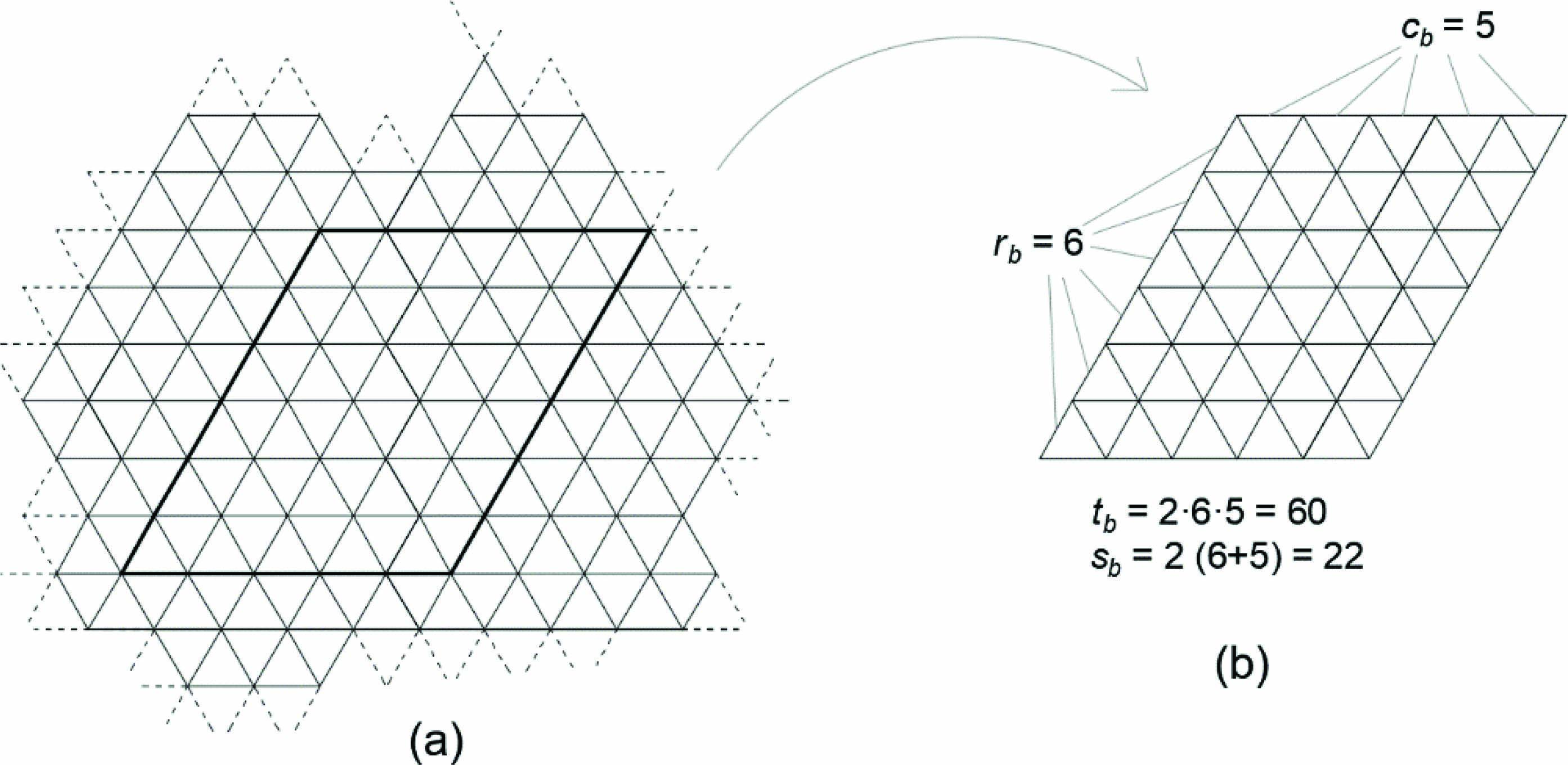
BIT is a portion of unbounded isotropic triangulation. The latter extends to infinite, i.e. presents no boundary edges, all angles are sixty degrees, all nodes valences are six and all triangles are the same size (Figure C.1(a)). The former is bounded by four edges forming a rhomboid (Figure C.1(b)), therefore not all valences are six, however sizes and angles are preserved as ideal isotropic. Parameters that characterize the BIT are the number of rows and columns, designated as $r_b$ and $c_b$. Figure C.1 provides one example.

Figure C.1 Ideal isotropic triangulation (a) and extraction of 6 $\times$ 5 BIT (b).

The number of triangles ($t_b$) and number contour segments ($s_b$) of BIT are computed from $r_b$ and $c_b$ as shown in Equations (C.1) and (C.2).

$$t_b=2r_b{c}_b$$

(C.1)

$$s_b=2(r_b+c_b)$$

(C.2)

As mention, BIT has all angles equal to sixty degrees and all triangles are the same size, but not all vertexes valences are six. Vertexes valences are calculated as per Table C.1.

Table C.1 Frequency (number of instances) of vertexes valences

Valence	Frequency
1	2
2	2
3	$2((c_b-1)+(r_b-1))$
4	0
5	0
6	$(c_b-1)\times (r_b-1)$

C.2 Computation of BIT Corresponding to Any Triangulation (AT)

Given AT mesh we can find its corresponding BIT using Equations (C.1) and (C.2). By manipulation of them we arrive to expressions (C.3).

$$\begin{array}{c}{r}_b=\frac{s_a}{4}+\sqrt{\frac{s_a{}^2}{16}-\frac{t_a}{2}}\hfill \\ s_b=\frac{s_a}{4}-\sqrt{\frac{s_a{}^2}{16}-\frac{t_a}{2}}\hfill \end{array}$$

(C.3)

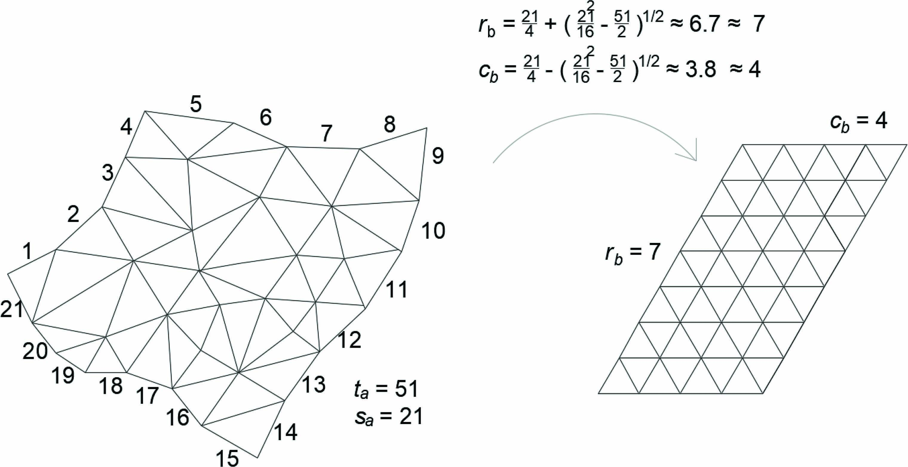
In Equations (C.3) we input the AT number of triangles and edge segments ($t_a$ and $s_a$) and obtain its corresponding BIT number of rows and columns ($r_b$ and $c_b$) and afterwards the BIT vertexes valences frequency as per Table C.1. Figure C.2 provides one example of the BIT associated to AT.

BIT is the closest version of AT to an ideal isotropic triangulation, then the closest the parameters (angles, sizes and valences) of AT are to its BIT the higher quality presents the former.

Figure C.2 Computation of BIT (right) for a given AT (left). Contour segments of AT are numbered.

Appendix D: Data for Numerical Examples

Example 7.1: Single Surface

Table D.1 QIT inputs

	Threshold	Tolerance for	Tolerance for	Tolerance for
$R$	distance to edge	curves (%)	surfaces (%)	derivatives (%)
12 and 6	4 and 2	1.0	4.0	15.0

Table D.2 Surface NURBS features

No. control points	$n=6\mathit{\hspace{1em}}m=5$
Degrees	$p=2\mathit{\hspace{1em}}q=2$
Knot vectors	$\Xi =\left\{\mathrm{000\hspace{0.25em}0.25\hspace{0.25em}0.50\hspace{0.25em}0.75\hspace{0.25em}111}\right\}$
	$H=\left\{\mathrm{000\hspace{0.25em}0.50\hspace{0.25em}0.50\hspace{0.25em}111}\right\}$

Table D.3 Control points coordinates and weights

	1	2	3	4	5
1	0, 0, $-$90, 1	0, 0, 0, 0.707	0, 30, 0, 1	0, 60, 0, 0.707	0, 60, $-$30, 1
2	30, 0, $-$15, 1	30, 15, 0, 1	30, 30, 0, 1	30, 45, 0, 1	30, 60, $-$15, 1
3	95, 0, 0, 1	95, 15, 0, 1	95, 30, 0, 1	95, 45, 0, 1	95, 60, 0, 1
4	150, 0, 0, 6	137.5, 15, 0, 1	125, 30, 0, 1	112.5, 45, 0, 1	100, 60, 0, 1
5	150, 65, 0, 1	137.5, 65, 0, 1	125, 65, 0, 1	112.5, 65, 0, 1	100, 65, 0, 1
6	150, 100, 0, 1	137.5, 100, 0, 1	125, 100, 0, 1	112.5, 100, 0, 1	100, 100, 0, 1

Example 7.2: Three Contiguous Surfaces

Table D.4 QIT inputs

	Threshold	Tolerance for	Tolerance for	Tolerance for
$R$	distance to edge	curves (%)	surfaces (%)	derivatives (%)
5	1.67	1.0	4.0	15.0

– Bottom surface:

Table D.5 Surface NURBS features

No. control points	$n=3\mathit{\hspace{1em}}m=5$
Degrees	$p=2\mathit{\hspace{1em}}q=2$
Knot vectors	$\Xi =\{\mathrm{000\hspace{0.25em}\hspace{0.25em}111}\}$
	$H=\{\mathrm{000\hspace{0.25em}0.50\hspace{0.25em}0.50\hspace{0.25em}111}\}$

Table D.6 Control points coordinates and weights

	1	2	3	4	5
1	108, 40, 0, 1	108, -28, 0, 0.707	40, -28, 0, 1	-28,-28, 0, 0.707	-28, 40, 0, 1
2	80, 40, 75, 1	80, 0, 75, 0.707	40, 0, 75, 1	0, 0, 75, 0.707	0, 40, 75, 1
3	80, 40, 150, 1	80, 0, 150, 0.707	40, 0, 150, 1	0, 0, 150, 0.707	0, 40, 150, 1

– Mid surface:

Table D.7 Surface NURBS features

No. control points	$n=5\mathit{\hspace{1em}}m=2$
Degrees	$p=2\mathit{\hspace{1em}}q=1$
Knot vectors	$\Xi =\{\mathrm{000\hspace{0.25em}0.50\hspace{0.25em}0.50\hspace{0.25em}111}\}$
	$H=\{\mathrm{00\hspace{0.25em}\hspace{0.25em}11}\}$

Table D.8 Control points coordinates and weights

	1	2
1	0, 40, 150, 1	20, 40, 150, 1
2	0, 0, 150, 0.707	20, 20, 150, 0.707
3	40, 0, 150, 1	40, 20, 150, 1
4	80, 0, 150, 0.707	60, 20, 150, 0.707
5	80, 40, 150, 1	60, 40, 150, 1

– Top surface:

Table D.9 Surface NURBS features

No. control points	$n=3\mathit{\hspace{1em}}m=5$
Degrees	$p=2\mathit{\hspace{1em}}q=2$
Knot vectors	$\Xi =\{\mathrm{000\hspace{0.25em}\hspace{0.25em}111}\}$
	$H=\{\mathrm{000\hspace{0.25em}0.50\hspace{0.25em}0.50\hspace{0.25em}111}\}$

Table D.10 Control points coordinates and weights

	1	2	3	4	5
1	60, 40, 150, 1	60, 20, 150,	40, 20, 150, 1	20, 20, 150, 0.707	20, 40, 150, 1
		0.707
2	60, 40, 210,	60, 20, 230,	40, 20, 230, 0.707	20, 20, 230, 0.707	20, 40, 210, 1
	0.707	0.50
3	60, 100, 210, 1	60, 100, 230,	40, 100, 230, 1	20, 100, 230, 0.707	20, 100, 210, 1
		0.707

Notes

¹We refer to B-spline as spline for brevity.

References

[1] T.J.R. Hughes, J.A. Cottrell, Y. Bazilevs, ‘Isogeometric analysis: CAD, finite elements, NURBS, exact geometry and mesh refinement’. Computer Methods in Applied Mechanics and Engineering, 194(39), pp. 4135–4195, 2005

[2] J.A. Cottrell, T.J.R. Hughes, Y. Bazilevs, ‘Isogeometric analysis: toward integration of CAD and FEA’, Oxford: Wiley, 2009.

[3] T.J. Baker, ‘Mesh generation: Art or science?’, Progress in Aerospace Sciences, 41(1), pp. 29–63, 2005.

[4] K. Shimada, ‘Current issues and trends in meshing and geometric processing for computational engineering analyses’, Journal of Computing and Information Science in Engineering, 11(2), pp. 021008, 2011.

[5] Q. Du, V. Faber, M. Gunzburger, ‘Centroidal Voronoi tessellations: Applications and algorithms’, SIAM Review, 41(4), pp. 637–676, 1999.

[6] P.J. Frey, H. Borouchaki, P. George, ‘3D Delaunay mesh generation coupled with an advancing-front approach’, Computer Methods in Applied Mechanics and Engineering, 157(1-2), pp. 115–131, 1998.

[7] R. Löhner, P. Parikh, ‘Generation of three-dimensional unstructured grids by the advancing-front method’, International Journal for Numerical Methods in Fluids, 8(10), pp. 1135–1149, 1988.

[8] K. Nakahashi, D. Sharov, ’Direct surface triangulation using the advancing front method’, 12th Computational Fluid Dynamics Conference 1995, pp. 1686, 1995.

[9] J.R. Tristano, S.J. Owen, S.A. Canann, ‘Advancing Front Surface Mesh Generation in Parametric Space Using a Riemannian Surface Definition’, IMR 1998, pp. 429–445, 1998.

[10] M.A. Yerry, M.S. Shephard, ‘Automatic three-dimensional mesh generation by the modified-octree technique’, International Journal for Numerical Methods in Engineering, 20(11), pp. 1965–1990, 1984.

[11] M.S. Shephard, M.K. Georges, ’Automatic three-dimensional mesh generation by the finite octree technique’, International Journal for Numerical Methods in Engineering, 32(4), pp. 709–749, 1991.

[12] X. Sheng, B.E. Hirsch, ‘Triangulation of trimmed surfaces in parametric space’, Computer-Aided Design, 24(8), pp. 437–444, 1992.

[13] H. Borouchaki, P. Laug, P. George, ‘Parametric surface meshing using a combined advancing-front generalized Delaunay approach’, International Journal for Numerical Methods in Engineering, 49(1–2), pp. 233–259, 2000.

[14] R.J. Cripps, S. Parwana, ‘A robust efficient tracing scheme for triangulating trimmed parametric surfaces’, Computer-Aided Design, 43(1), pp. 12–20, 2011.

[15] E. Béchet, J. Cuilliere, F Trochu, ‘Generation of a finite element MESH from stereolithography (STL) files’, Computer-Aided Design, 34(1), pp. 1–17, 2002.

[16] D. Wang, O. Hassan, K. Morgan, N. Weatherill, ’EQSM: An efficient high quality surface grid generation method based on remeshing’, Computer Methods in Applied Mechanics and Engineering, 195(41–43), pp. 5621–5633, 2006.

[17] S.W. Yang, Y. Choi, ’Triangulation of CAD data for visualization using a compact array-based triangle data structure’, Computers & Graphics, 34(4), pp. 424–429, 2010.

[18] E. Marchandise, J. Remacle, C. Geuzaine, ‘Optimal parametrizations for surface remeshing’, Engineering with Computers, 30(3), pp. 383–402, 2014.

[19] R. Aubry, S. Dey, E.L. Mestreau, B.K. Karamete, D. Gayman, ‘A robust conforming NURBS tessellation for industrial applications based on a mesh generation approach’, Computer-Aided Design, 63, pp. 26–38, 2015.

[20] J. Guo , F. Ding, X. Jia, D. Yan, ‘Automatic and high-quality surface mesh generation for CAD models’, Computer-Aided Design, 109, pp. 49–59, 2019.

[21] V. Surazhsky, P. Alliez, C. Gotsman, ‘Isotropic remeshing of surfaces: a local parameterization approach’, 2003.

[22] P. Alliez, E.C. De Verdire, O. Devillers, M. Isenburg, ’Isotropic surface remeshing’, 2003 Shape Modeling International. 2003, IEEE, pp. 49–5, 2003.

[23] S.W. Yang, Y. Choi, ‘Triangulation of CAD data for visualization using a compact array-based triangle data structure’, Computers & Graphics, 34(4), pp. 424–429, 2010.

[24] Y. Li, W. Wang, R. Ling, C. Tu, ‘Shape optimization of quad mesh elements’, Computers & Graphics, 35(3), pp. 444–451, 2011.

[25] M.S. Ebeida, A. Patney, J.D. Owens, E. Mestreau, ‘Isotropic conforming refinement of quadrilateral and hexahedral meshes using two-refinement templates’, International Journal for Numerical Methods in Engineering, 88(10), pp. 974–985, 2011.

[26] M. Tsai, C. Cheng, M. Cheng, ‘A real-time NURBS surface interpolator for precision three-axis CNC machining’, International Journal of Machine Tools and Manufacture, 43(12), pp. 1217–1227, 2003.

[27] P. Bézier, ‘Numerical control: mathematics and applications’, 1970.

[28] A.R. Forrest, ‘Interactive interpolation and approximation by Bézier polynomials’, The Computer Journal, 15(1), pp. 71–79, 1972.

[29] S. Bernstein, ‘Démonstration du théoreme de Weierstrass fondée sur le calcul des probabilities’, Comm.Soc.Math.Kharkov, 13, pp. 1–2, 1912.

[30] M.G. Cox, ‘The numerical evaluation of B-splines’, IMA Journal of Applied Mathematics, 10(2), pp. 134–149, 1972.

[31] C. De Boor, ‘On calculating with B-splines’, Journal of Approximation theory, 6(1), pp. 50–62, 1972.

[32] E. Isaacson, H.B. Keller, ‘Analysis of numerical methods’, John Wiley & Sons, 1966.

[33] S.C. Chapra, R.P. Canale, ‘Numerical methods for engineers’, Boston: McGraw-Hill Higher Education, 2010.

[34] L. Piegl, W. Tiller, ‘The NURBS Book’, 2 edn. Springer-Verlag, 1996.

Biographies

Daniel Herrero Adán is a Structural Engineer at Hydrock Consultants, Bristol, UK. He is a Ph.D. student at the University of the West of England Bristol (UK) since October 2015. He attended to the Technical University of Madrid, Spain, where he received the degrees in Forestry Engineering in 2003 and in Mechanical Engineering in 2009. In 2014 he obtained the Master degree in Mechanical Engineering in the University of Distance Learning, Spain. Through all these years he worked in the industry as Forestry, Mechanical and Structural Engineer in Spain and the UK. He is author of 4 papers, including journal and conference papers. His research areas of interest include computational mechanics, integration of CAD and analysis, Isogeometric Analysis of solids, optimization of structural design and plastic and dynamic analysis.

Rui Cardoso Senior Lecturer at Brunel University London. Published more than 80 papers in international journals and conferences. Published a book in September 2018 with title: Stress Analysis for Lightweight Structures: A Matlab Oriented Approach. Chair of Numisheet 2016, International Conference and Workshop on Numerical Simulation of 3D Sheet Metal Forming Processes, September 2016, Bristol, UK.

European Journal of Computational Mechanics, Vol. 29_1, 27–82.
doi: 10.13052/ejcm2642-2085.2912
© 2020 River Publishers