A Unified Corotational Framework for 2D Beams: Bridging the Crisfield and Krenk Formulations

William T. M. Silva^*, Éder L. R. Nascimento, Sebastião S. da Silva and A. Portela

Department of Civil and Environmental Engineering, University of Brasília, Brasília, Brazil
E-mail: taylor@unb.br; ederlrn@gmail.com; sebastiao_simao@yahoo.com.br; a3portela@gmail.com
*Corresponding Author

Received 16 July 2026; Accepted 11 August 2026

Abstract

This paper presentes a unified corotational framework for 2D beam elements that achieves a theoretical synthesis between the seminal formulations of Crisfield and Krenk. A central contribution of this research is the analytical demonstration that these two traditionally distinct approaches converge to an identical tangent stiffness matrix, offering a unified perspective on objective corotational kinematics. The framework is systematically applied to three fundamental kinematic theories: Euler-Bernoulli, Timoshenko, and shallow arch Euler-Bernoulli, demonstrating its versatility across different levels of structural refinement. By decomposing the motion into a global rigid-body component and a local deformational part, characterized by three degrees of freedom, the formulation effectively isolates the nonlinearities of the coordinate transformation. A robust numerical strategy utilizing a modulo function is implemented to resolve the $\pm 2\pi$ periodicity singularity, ensuring stable convergence during extreme rigid-body rotations. Internal forces and tangent stiffness matrices are derived via the principle of virtual work, providing a transparent and modular implementation for each beam theory. The accuracy and computational efficiency of the unified formulation are validated through a series of challenging numerical benchmarks involving the geometrically nonlinear analysis of beams, frames, and arches, featuring complex equilibrium paths with limit points and multiple snap-back loops. Comprehensive mesh convergence studies confirm that the shallow arch Euler-Bernoulli element, incorporating explicit axial-bending coupling, achieves superior accuracy and convergence efficiency in problems involving significant geometric nonlinearity.

Keywords: Geometrical nonlinear analysis, Corotational kinematics, Euler-Bernoulli beam element, Timoshenko beam element, Shallow arch Euler-Bernoulli beam element.

1 Introduction

The analysis of highly flexible structures such as offshore wind turbine blades, long-span bridges, and deployable space mechanisms, requires numerical formulations capable of capturing extreme geometric nonlinearities. In this context, the corotational method has emerged as one of the most efficient and elegant frameworks for nonlinear structural analysis [1, 2]. The fundamental principle of the corotational approach is the decomposition of the total motion into a global rigid-body component and a local deformational component. By isolating the rigid-body motion at the element level, the corotational framework allows for the use of high-performance linear finite element libraries to solve complex nonlinear problems, provided that the coordinate transformation is handled with kinematic objectivity.

Over the last few decades, two primary theoretical branches of the corotational method for planar beams have dominated the literature. The first, popularized by Crisfield [1], utilizes a projection-based approach that has become the standard for integrating linear elements into nonlinear solvers. The second, advanced by Krenk [2, 3, 4], employs an equilibrium-based format where stress states are described relative to the chord connecting the element nodes. While both frameworks are widely utilized and have been extended to include shear flexibility [5], curved geometries [6], and plastic hinges [7, 8], they are often presented as distinct or competing formulations in the literature.

The primary contribution of this paper is the theoretical unification of these two classical frameworks. We provide an analytical demonstration that, despite their different kinematic derivations, the Crisfield and Krenk approaches yield an identical tangent stiffness matrix. This synthesis not only clarifies a fundamental aspect of corotational theory but also provides a generalized platform for modular structural analysis, wherein different beam kinematics can be seamlessly integrated by replacing only the local elastic stiffness matrix ${\text{K}}_d$ while maintaining the same global geometric stiffness operator. This modularity enhances code maintainability and facilitates the incorporation of additional kinematic theories without reformulating the entire corotational machinery. By establishing this equivalence, we show that the choice between these formulations is a matter of implementation preference rather than theoretical divergence.

To demonstrate the versatility of this unified framework, we apply it to three distinct beam theories: the classical Euler-Bernoulli (EB) beam, the shear-flexible Timoshenko (TI) beam, and the shallow arch Euler-Bernoulli (SAB) element. The latter is particularly significant, as it accounts for the coupling between axial and bending strains, which is essential for the precision of arch and frame analysis under significant deformation [9]. While the primary contribution of this work is theoretical, establishing the mathematical equivalence between two seminal formulations, the unified framework offers practical advantages in terms of computational modularity, pedagogical clarity, and the systematic integration of diverse beam theories within a single implementation.

Furthermore, this work addresses a persistent numerical challenge in corotational kinematics: the singularity associated with large rigid-body rotations. While the corotational method is inherently designed for large displacements, rotations that are multiples of $\pm \pi$ can lead to numerical divergence in standard iterative solvers. We implement a robust numerical strategy utilizing a modulo function [10] to ensure the continuity of the rotational variables, allowing for the simulation of structures undergoing multiple full revolutions without loss of convergence.

The paper is organized as follows: Section 2 describes the unified corotational kinematics and the proof of equivalence between the Crisfield and Krenk formulations. Sections 3, 4 and 5 details the derivation of the internal force vectors and tangent stiffness matrices for the EB, TI, and SAB elements, respectively. Finally, Section 6 validates the robustness and accuracy of the unified formulation through a series of challenging benchmarks.

2 Corotational Kinematics

The corotational kinematics presented in this section primarily follows the framework proposed by Crisfield [1]. Figure 1 illustrates the kinematic variables employed in the corotational description of the 2D beam element. The nodal coordinates of the element in the reference configuration are $(X_1,Y_1)$ and $(X_2,Y_2)$, respectively. In the deformed configuration, these coordinates are defined as $(x_1,y_1)$ and $(x_2,y_2)$. Each element is associated with a local reference coordinate system $(x_e,y_e)$, which is used to define the deformational component of the motion. The global displacement vector ${\text{u}}_g$ and the local deformational displacement vector ${\text{u}}_d$ are defined as:

$${\text{u}}_g={(u_1,v_1,{\theta }_1,u_2,v_2,{\theta }_2)}^{{}^T},{\text{u}}_d={(\overline{u},{\overline{\theta }}_1,{\overline{\theta }}_2)}^{{}^T}$$

(1)

where $\overline{u}$ represents the relative displacement between nodes 1 and 2 along the local $x_e$ axis, while ${\overline{\theta }}_1$ and ${\overline{\theta }}_2$ denote the deformational rotations of nodes 1 and 2, respectively. The components of the vector ${\text{u}}_d$ are given by:

$$\overline{u}=l-l_0,{\overline{\theta }}_1={\theta }_1-\alpha ,{\overline{\theta }}_2={\theta }_2-\alpha$$

(2)

In these expressions, $l_0$ and $l$ represent the initial and current lengths of the element, respectively, defined as:

$$\begin{array}{c}{l}_0=\sqrt{X_{21}^{{}^2}+Y_{21}^{{}^2}},l=\sqrt{{(X_{21}+u_{21})}^{{}^2}+{(Y_{21}+v_{21})}^{{}^2}}\\ \\ X_{21}=X_2-X_1,Y_{21}=Y_2-Y_1,u_{21}=u_2-u_1,v_{21}=v_2-v_1\end{array}$$

(3)

As shown in Figure 1, $\alpha =\beta -{\beta }_0$ defines the rigid body rotation of the element, calculated through:

$$\mathrm{sen}\alpha =\cos {\beta }_0\mathrm{sen}\beta -\mathrm{sen}{\beta }_0\cos \beta ,\cos \alpha =\cos {\beta }_0\cos \beta +\mathrm{sen}{\beta }_0\mathrm{sen}\beta$$

(4)

where ${\beta }_0$ is initial slope of the element and $\beta$ is the slope of the line connecting the two nodes in the current configuration. These angles are determined as:

$$\cos {\beta }_0=\frac{X_{21}}{l_0},\mathrm{sen}{\beta }_0=\frac{Y_{21}}{l_0},\cos \beta =\frac{X_{21}+u_{21}}{l}=\frac{x_{21}}{l},\mathrm{sen}\beta =\frac{Y_{21}+v_{21}}{l}=\frac{y_{21}}{l}$$

(5)

By substituting Equation (5) into Equation (4), we obtain:

$$\begin{array}{c}\cos \alpha =\frac{x_{21}^{\ast }}{l_{0}l},\mathrm{sen}\alpha =\frac{y_{21}^{\ast }}{l_{0}l}\\ \\ x_{21}^{\ast }=X_{21}{x}_{21}+Y_{21}{y}_{21},y_{21}^{\ast }=X_{21}{y}_{21}-Y_{21}{x}_{21}\end{array}$$

(6)

where $x_{21}^{\ast }$ and $y_{21}^{\ast }$ relate to the differences in nodal translations in the $x$ and $y$ directions. Utilizing the relationship $\tan \frac{\alpha }{2}=\frac{1-\cos \alpha }{\sin \alpha }$, the rigid body rotation is expressed as:

$$\alpha =2\mathrm{t}\mathrm{a}{\mathrm{n}}^{-1}\left(\frac{1-\cos \alpha }{\mathrm{sen}\alpha }\right)=2\mathrm{t}\mathrm{a}{\mathrm{n}}^{-1}\left(\frac{l_{0}l-x_{21}^{\ast }}{y_{21}^{\ast }}\right)$$

(7)

This expression is singular if $y_{21}^{\ast }=0$, implying $\alpha =0$ if $x_{21}^{\ast }=l_{0}l$, or $\alpha =\pi$ if $x_{21}^{\ast }=-l_{0}l$. To accommodate large rotations, the nodal deformational rotations are calculate using the modulo function [10]:

$${\overline{\theta }}_1=\underset{2\pi }{\mathrm{mod}}(({\theta }_1-\alpha )+\pi )-\pi ,{\overline{\theta }}_2=\underset{2\pi }{\mathrm{mod}}(({\theta }_2-\alpha )+\pi )-\pi$$

(8)

The modulo function yields values in the range $[0,2\pi [$, and the final term shifts the interval to $[-\pi ,\pi ]$ to maintain symmetry about zero. This step is essential to prevent numerical divergence when the element undergoes rotations that are multiples of $\pm \pi$.

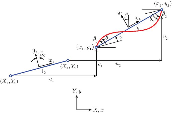
Figure 1 Motion of 2D beam element.

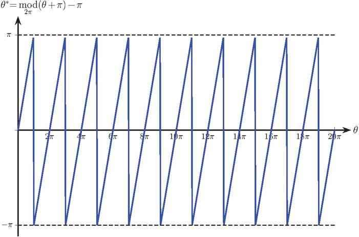
Figure 2 Application of the modulo function for large rotations.

Figure 2 illustrates the modulo function for angles in the interval $[0,20\pi [$, corresponding to 10 complete revolutions. Note that the resulting values ${\theta }^{{}^{\ast }}$ remain constrained within $[-\pi ,\pi ]$.

Virtual local displacements are obtained by differentiating Equation (2):

$$\begin{array}{cc}\hfill \delta \overline{u}=& \delta l={(-\cos \beta ,-\mathrm{sen}\beta ,0,\cos \beta ,\mathrm{sen}\beta ,0)}^{{}^T}\delta {\text{u}}_g\hfill \\ \multicolumn{2}{c}{}\\ \hfill \delta {\overline{\theta }}_1=& \delta {\theta }_1-\delta \alpha =\delta {\theta }_1-\delta \beta \hfill \\ \multicolumn{2}{c}{}\\ \hfill \delta {\overline{\theta }}_2=& \delta {\theta }_2-\delta \alpha =\delta {\theta }_2-\delta \beta \hfill \end{array}$$

(9)

The virtual variation of $\beta$ is found by differentiating Equation (5) with respect to global displacements:

$$\delta \beta =\frac{1}{l}{(\mathrm{sen}\beta ,-\cos \beta ,0,-\mathrm{sen}\beta ,\cos \beta ,0)}^{{}^T}\delta {\text{u}}_g$$

(10)

The transformation matrix B, relating the virtual variations of local and global variables, is defined as:

$$\begin{array}{c}\delta {\text{u}}_d=\text{B}\delta {\text{u}}_g\\ \\ \text{B}=\left[\begin{array}{cccccc}-\cos \beta & -\mathrm{sen}\beta & 0& \cos \beta & \mathrm{sen}\beta & 0\\ \\ -\frac{\mathrm{sen}\beta }{l}& \frac{\cos \beta }{l}& 1& \frac{\mathrm{sen}\beta }{l}& -\frac{\cos \beta }{l}& 0\\ \\ -\frac{\mathrm{sen}\beta }{l}& \frac{\cos \beta }{l}& 0& \frac{\mathrm{sen}\beta }{l}& -\frac{\cos \beta }{l}& 1\end{array}\right]\end{array}$$

(11)

The relationship between the local internal force vector ${\text{f}}_d$ and the global counterpart ${\text{f}}_g$ is established by equating the virtual work in both systems:

$$V=\delta {\text{u}}_g^T{\text{f}}_g=\delta {\text{u}}_d^T{\text{f}}_d=\delta {\text{u}}_g^T{\text{B}}^{{}^T}{\text{f}}_d$$

(12)

Since Equation (12) must hold for any arbitrary $\delta {\text{u}}_g$, the global internal force vector is given by:

$${\text{f}}_g={\text{B}}^{{}^T}{\text{f}}_d$$

(13)

where ${\text{f}}_d={(n,m_1,m_2)}^{{}^T}$ depends on the element’s specific beam theory. In the subsequent sections, the equivalence between the corotational formulations of Crisfield [1] and Krenk [2] will be demonstrated for the 2D case.

2.1 Nodal Force Vector in Local and Global Coordinates

The following development regarding nodal forces is primarily based on Krenk [2]. Figure 3 depicts the nodal force vectors in global and local coordinates. The relationship between the local internal force vector and the nodal force in local coordinates is established via the equilibrium matrix S:

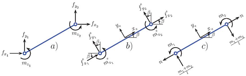
Figure 3 Nodal force vectors in (a) global coordinates, (b) local coordinates, and (c) the local internal force vector.

$$\begin{array}{c}{\text{f}}_e=\text{S}{\text{f}}_d\\ \\ \text{S}=\left[\begin{array}{ccc}-1& 0& 0\\ \\ 0& 1/l& 1/l\\ \\ 0& 1& 0\\ \\ 1& 0& 0\\ \\ 0& -1/l& -1/l\\ \\ 0& 0& 1\end{array}\right]\end{array}$$

(14)

A primary similarity between the descriptions of Crisfield and Krenk is observed by setting $\beta =0$ in Equation (11), which yields ${\text{B}}^{{}^T}=\text{S}$. The relationship between the nodal force vectors in local and global coordinates is given by:

$$\begin{array}{c}{\text{f}}_g=\text{R}{\text{f}}_e\\ \\ \text{R}=\left[\begin{array}{cccccc}\cos \beta & -\mathrm{sen}\beta & 0& 0& 0& 0\\ \\ \mathrm{sen}\beta & \cos \beta & 0& 0& 0& 0\\ \\ 0& 0& 1& 0& 0& 0\\ \\ 0& 0& 0& \cos \beta & -\mathrm{sen}\beta & 0\\ \\ 0& 0& 0& \mathrm{sen}\beta & \cos \beta & 0\\ \\ 0& 0& 0& 0& 0& 1\end{array}\right]\end{array}$$

(15)

where R is the rotation matrix. Substituting Equation (14) into Equation (15), we obtain:

$${\text{f}}_g=\text{R}\text{S}{\text{f}}_d$$

(16)

Comparing Equations (13) and (16) reveals a second similarity: ${\text{B}}^{{}^T}=\text{R}\text{S}$ for any value of $\beta$.

2.2 Tangent Stiffness Matrix in Global Coordinates

Returning to Crisfield’s formulation, the relationship between the global nodal force and displacement increments is defined as:

$$\delta {\text{f}}_g=\text{K}\delta {\text{u}}_g$$

(17)

where K is the global tangent stiffness matrix. This matrix is obtained by differentiating Equation (13):

$$\delta {\text{f}}_g={\text{B}}^{{}^T}\delta {\text{f}}_d+\delta {\text{B}}^{{}^T}{\text{f}}_d={\text{B}}^{{}^T}\delta {\text{f}}_d+n\delta {\text{b}}_1+m_1\delta {\text{b}}_2+m_2\delta {\text{b}}_3$$

(18)

In this context, ${\text{b}}_1$, ${\text{b}}_2$ and ${\text{b}}_3$ are the columns of ${\text{B}}^{{}^T}$. To facilitate the derivation, we define the auxiliary vectors:

$$\begin{array}{cc}\hfill \text{r}=& {(-\cos \beta ,-\mathrm{sen}\beta ,0,\cos \beta ,\mathrm{sen}\beta ,0)}^{{}^T}\hfill \\ \multicolumn{2}{c}{}\\ \hfill \text{z}=& {(\mathrm{sen}\beta ,-\cos \beta ,0,-\mathrm{sen}\beta ,\cos \beta ,0)}^{{}^T}\hfill \end{array}$$

(19)

with virtual variations:

$$\delta \text{r}=\text{z}\delta \beta ,\delta \text{z}=-\text{r}\delta \beta$$

(20)

Consequently, Equations (9) and (10) can be rewritten as:

$$\delta \overline{u}=\delta l={\text{r}}^T\delta {\text{u}}_g,\delta \beta \frac{1}{l}{\text{z}}^T\delta {\text{u}}_g$$

(21)

The vectors ${\text{b}}_i$ are then:

$$\begin{array}{cc}\hfill {\text{b}}_1=& \text{r}\hfill \\ \multicolumn{2}{c}{}\\ \hfill {\text{b}}_2=& {(0,0,1,0,0,0)}^{{}^T}-\frac{1}{l}\text{z}\hfill \\ \multicolumn{2}{c}{}\\ \hfill {\text{b}}_3=& {(0,0,0,0,0,1)}^{{}^T}-\frac{1}{l}\text{z}\hfill \end{array}$$

(22)

and their variations are:

$$\begin{array}{cc}\hfill \delta {\text{b}}_1=& \delta \text{r}=\frac{1}{l}(\text{z}\otimes \text{z})\delta {\text{u}}_g\hfill \\ \multicolumn{2}{c}{}\\ \hfill \delta {\text{b}}_2=& \delta {\text{b}}_3=-\frac{1}{l}\delta \text{z}+\frac{\delta l}{l^{{}^2}}\text{z}=\frac{1}{l^{{}^2}}(\text{r}\otimes \text{z}+\text{z}\otimes \text{r})\delta {\text{u}}_g\hfill \end{array}$$

(23)

Assuming that ${\text{f}}_d={\text{K}}_d{\text{u}}_d\Rightarrow \delta {\text{f}}_d={\text{K}}_d\delta {\text{u}}_d={\text{K}}_d\text{B}\delta {\text{u}}_g$, where ${\text{K}}_d$ is the elastic stiffness matrix, which depends of the type of beam element adopted. Finally, from the Equations (18) and (23), the global tangent stiffness matrix is obtained as:

$$\text{K}={\text{B}}^{{}^T}{\text{K}}_d\text{B}+\frac{n}{l}(\text{z}\otimes \text{z})+\frac{1}{l^{{}^2}}(m_1+m_2)(\text{r}\otimes \text{z}+\text{z}\otimes \text{r})$$

(24)

The first term represents the material stiffness matrix. Noting that the shear force is $Q=\frac{m_1+m_2}{l}$, as set out in Figure 3(c), the global geometric stiffness matrix becomes:

$${\text{K}}_g=\frac{N}{l}(\text{z}\otimes \text{z})+\frac{Q}{l}(\text{r}\otimes \text{z}+\text{z}\otimes \text{r})$$

(25)

2.3 Tangent Stiffness Matrix in Local Coordinates

The nonlinear modeling in this section utilizes Krenk’s formulation. The relationship between virtual force and displacement increments in local coordinates is:

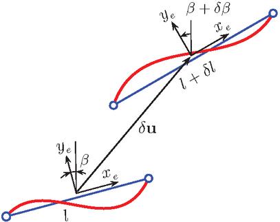
Figure 4 Incremental motion of the 2D beam element.

$$\delta {\text{f}}_e={\text{K}}_e\delta {\text{u}}_e$$

(26)

Considering the current configuration in Figure 4, virtual variations in rigid body rotation and length are:

$$\delta \beta =\frac{\delta v_2^e-\delta v_1^e}{l},\delta l=\delta u_2^e-\delta u_1^e$$

(27)

Based on the principle of virtual work, the virtual variation of the internal work is expressed as:

$$\delta V=\delta {\text{u}}_e^T{\text{f}}_e=\delta {\text{u}}_e^T\text{S}{\text{f}}_d=\delta {\text{u}}_d^T{\text{f}}_d$$

(28)

which implies the kinematic relationship $\delta {\text{u}}_d={\text{S}}^{{}^T}\delta {\text{u}}_e$. The variation of the global force vector (Equation 16) is subsequently derived as:

$$\begin{array}{c}\delta {\text{f}}_g=\text{R}\text{S}\delta {\text{f}}_d+\text{R}\delta \text{S}{\text{f}}_d+\delta \text{R}\text{S}{\text{f}}_d\\ \\ \delta \text{R}=\left[\begin{array}{cccccc}-\sin \beta & -\cos \beta & 0& 0& 0& 0\\ \\ \cos \beta & -\sin \beta & 0& 0& 0& 0\\ \\ 0& 0& 0& 0& 0& 0\\ \\ 0& 0& 0& -\sin \beta & -\cos \beta & 0\\ \\ 0& 0& 0& \cos \beta & -\sin \beta & 0\\ \\ 0& 0& 0& 0& 0& 0\end{array}\right]\delta \beta \\ \\ \delta \text{S}=\left[\begin{array}{ccc}0& 0& 0\\ \\ 0& -1/l^{{}^2}& -1/l^{{}^2}\\ \\ 0& 0& 0\\ \\ 0& 0& 0\\ \\ 0& 1/l^{{}^2}& 1/l^{{}^2}\\ \\ 0& 0& 0\end{array}\right]\delta l\end{array}$$

(29)

Noting that $\delta {\text{f}}_d={\text{K}}_d\delta {\text{u}}_d\Rightarrow \delta {\text{f}}_d={\text{K}}_d{\text{S}}^{{}^T}\delta {\text{u}}_e$ and invoking Equation (15), Equation (29) can be reformulated in local coordinates as:

$$\delta {\text{f}}_e={\text{S}\text{K}}_d{\text{S}}^{{}^T}\delta {\text{u}}_e+(\delta \text{S}+{\text{R}}^{{}^T}\delta \text{R}\text{S}){\text{f}}_d$$

(30)

Finally, according to Equation (26), the tangent stiffness matrix in local coordinates is given by:

$${\text{K}}_e={\text{S}\text{K}}_d{\text{S}}^{{}^T}+{\text{K}}_r$$

(31)

where the first term represents the material stiffness matrix, while ${\text{K}}_r$ is the corotational stiffness matrix. This matrix represents the effects of rigid body rotation variations and shear force changes due to length variations, which according to Equation (30) implies ${\text{K}}_r\delta {\text{u}}_e=(\delta \text{S}+{\text{R}}^{{}^T}\delta \text{R}\text{S}){\text{f}}_d$. Taking into account Equations (15), (27) and (29), following algebraic development yields:

$${\text{K}}_r=\frac{1}{l}\left[\begin{array}{cccccc}0& Q& 0& 0& -Q& 0\\ \\ Q& N& 0& -Q& -N& 0\\ \\ 0& 0& 0& 0& 0& 0\\ \\ 0& -Q& 0& 0& Q& 0\\ \\ -Q& -N& 0& Q& N& 0\\ \\ 0& 0& 0& 0& 0& 0\end{array}\right]$$

(32)

It is important to emphasize that the equivalence demonstrated here is not merely approximate or asymptotic; the tangent stiffness matrices in global coordinates are algebraically identical for both formulations, regardless of the magnitude of rigid-body rotations or deformations. This identity holds for any value of the rotation angle $\beta$ and for arbitrarily large displacements. Consequently, numerical results obtained using the unified framework presented herein are indistinguishable from those obtained using faithful implementations of either Crisfield’s or Krenk’s original formulations, provided the same local beam theory (${\text{K}}_d$) is employed. Any observed differences in computational results would stem solely from implementation details (e.g., convergence tolerances, step-size control strategies) rather than from theoretical divergence. This matrix constitutes a fundamental portion of the complete geometric stiffness matrix (see [5]). A third similarity is established by the equality of ${\text{K}}_r$ (Equation 32) and ${\text{K}}_g$ (Equation 25) when $\beta =0$. For this case, the auxiliary vectors in Equation (19) can be rewritten as:

$$\begin{array}{cc}\hfill \text{r}={(-1,0,0,1,0,0)}^T={(-{\text{e}}_1,{\text{e}}_1)}^T& \\ \multicolumn{2}{c}{}\\ \hfill \text{z}={(0,-1,0,0,1,0)}^T={(-{\text{e}}_2,{\text{e}}_2)}^T& \end{array}$$

(33)

Substituting Equation (33) into Equation (25), we arrive at:

$${\text{K}}_g=\frac{n}{l}\left(\left\{\begin{array}{c}-{\text{e}}_2\\ {\text{e}}_2\end{array}\right\}\otimes \left\{\begin{array}{c}-{\text{e}}_2\\ {\text{e}}_2\end{array}\right\}\right)+\frac{Q}{l}\left(\left\{\begin{array}{c}-{\text{e}}_1\\ {\text{e}}_1\end{array}\right\}\otimes \left\{\begin{array}{c}-{\text{e}}_2\\ {\text{e}}_2\end{array}\right\}+\left\{\begin{array}{c}-{\text{e}}_2\\ {\text{e}}_2\end{array}\right\}\otimes \left\{\begin{array}{c}-{\text{e}}_1\\ {\text{e}}_1\end{array}\right\}\right)$$

(34)

Algebraic expansion of Equation (34) leads directly to ${\text{K}}_r$ in Equation (32). Indeed, for $\beta =0$, Krenk’s formulation emerges as a specific instance of Crisfield’s.

A fourth similarity is described hereafter. Taking Equation (31) into account, the tangent stiffness matrix in global coordinates, $\text{K}={\text{R}\text{K}}_e{\text{R}}^{{}^T}$, within Krenk’s formulation is defined as

$$\text{K}={\text{R}\text{S}\text{K}}_d{\text{S}}^{{}^T}{\text{R}}^{{}^T}+{\text{R}\text{K}}_r{\text{R}}^{{}^T}$$

(35)

where the first term represents the material stiffness matrix, while the second term represents the geometric stiffness matrix. Through the identity ${\text{B}}^{{}^T}=\text{R}\text{S}$ defined in Section 2.1, it can be demonstrated that

$$\begin{array}{c}{\text{R}\text{S}\text{K}}_d{\text{S}}^{{}^T}{\text{R}}^{{}^T}={\text{B}}^{{}^T}{\text{K}}_d\text{B}\\ \\ {\text{R}\text{K}}_r{\text{R}}^{{}^T}=\frac{N}{l}(\text{z}\otimes \text{z})+\frac{Q}{l}(\text{r}\otimes \text{z}+\text{z}\otimes \text{r})\end{array}$$

(36)

for any value of $\beta$. Consequently, both formulations yield identical tangent stiffness matrices in global coordinates.

In summary, the four fundamental similarities established in this section, namely

$$\begin{array}{cc}(1){\text{B}}^{{}^T}=\text{S}\text{when}\beta =0,\hfill & (2){\text{B}}^{{}^T}=\text{R}\text{S}\text{for any}\beta ,\hfill \\ \multicolumn{2}{c}{}\\ (3){\text{K}}_r={\text{K}}_g\text{when}\beta =0,\hfill & (4){\text{R}\text{K}}_e{\text{R}}^{{}^T}=\text{K}\text{for any}\beta ,\hfill \end{array}$$

(37)

collectively demonstrate the complete theoretical unification of the Crisfield and Krenk corotational frameworks for planar beam elements. This unification validates the assertion that the choice between these formulations is one of implementation preference rather than fundamental theoretical distinction.

Finally, the elastic stiffness matrix ${\text{K}}_d$ is derived by differentiating the internal forces ${\text{f}}_d$ with respect to the deformational displacements ${\text{u}}_d$:

$${\text{K}}_d=\left[\begin{array}{ccc}\frac{\partial n}{\partial \overline{u}}& \frac{\partial n}{\partial {\overline{\theta }}_1}& \frac{\partial n}{\partial {\overline{\theta }}_2}\\ \\ \frac{\partial m_1}{\partial \overline{u}}& \frac{\partial m_1}{\partial {\overline{\theta }}_1}& \frac{\partial m_1}{\partial {\overline{\theta }}_2}\\ \\ \frac{\partial m_2}{\partial \overline{u}}& \frac{\partial m_2}{\partial {\overline{\theta }}_1}& \frac{\partial m_2}{\partial {\overline{\theta }}_2}\end{array}\right]$$

(38)

The following sections detail the derivation of ${\text{K}}_d$ for Euler-Bernoulli, Timoshenko, and shallow arch Euler-Bernoulli beam elements.

3 Euler-Bernoulli Element

The deformational motion of the Euler-Bernoulli beam element is described by the following shape functions:

$$u=\frac{x}{l_0}\overline{u},v=x{\left(1-\frac{x}{l_0}\right)}^{{}^2}{\overline{\theta }}_1+\frac{x^2}{l_0}\left(\frac{x}{l_0}-1\right){\overline{\theta }}_2$$

(39)

It is important to note that the transverse nodal displacements $v_1$ and $v_2$ vanish because the shape functions are defined with respect to the local coordinates in the current configuration, as illustrated in Figure 1. Consequently, the curvature and longitudinal strain deformation at any point within the element are defined as:

$$\begin{array}{cc}\hfill \kappa =& \frac{{\partial }^{2}v}{\partial x^2}=\left(-\frac{4}{l_0}+6\frac{x}{l_0^{{}^2}}\right){\overline{\theta }}_1+\left(-\frac{2}{l_0}+6\frac{x}{l_0^{{}^2}}\right){\overline{\theta }}_2\hfill \\ \multicolumn{2}{c}{}\\ \hfill \epsilon =& \frac{\partial u}{\partial x}-\kappa y=\frac{\overline{u}}{l_0}+y\left(\left(\frac{4}{l_0}-6\frac{x}{l_0^{{}^2}}\right){\overline{\theta }}_1+\left(\frac{2}{l_0}-6\frac{x}{l_0^{{}^2}}\right){\overline{\theta }}_2\right)\hfill \end{array}$$

(40)

By applying a virtual variation to the local displacement vector $(\delta \overline{u},\delta {\overline{\theta }}_1,\delta {\overline{\theta }}_2)$, a virtual variation of the strain field $\delta \epsilon$ is induced. According to the principle of virtual works, we have:

$$\begin{array}{c}\delta V=\underset{V}{\int }\sigma \delta \epsilon \mathit{d}V=n\delta \overline{u}+m_1\delta {\overline{\theta }}_1+m_2\delta {\overline{\theta }}_2\\ \\ n=\underset{A}{\int }\sigma \mathit{d}A,m_1=\underset{A}{\int }\sigma y\mathit{d}A,m_2=-\underset{A}{\int }\sigma y\mathit{d}A\end{array}$$

(41)

Assuming a linear elastic constitutive relation $\sigma =E\epsilon$ and substituting Equation (40) in the relations established in Equation (41), the local internal force vector is obtained as:

$${\text{f}}_l=\left\{\begin{array}{c}n\\ \\ m_1\\ \\ m_2\end{array}\right\}=\left\{\begin{array}{c}\frac{EA}{l_o}\overline{u}\\ \\ \frac{EI}{l_o}(4{\overline{\theta }}_1+2{\overline{\theta }}_2)\\ \\ \frac{EI}{l_o}(4{\overline{\theta }}_2+2{\overline{\theta }}_1)\end{array}\right\}$$

(42)

Finally, by differentiating each component of the internal force vector in Equation (42) with respect to the local displacements $(\overline{u},{\overline{\theta }}_1,{\overline{\theta }}_2)$, the elastic stiffness matrix is derived as:

$${\text{K}}_d=\left[\begin{array}{ccc}\frac{EA}{l_o}& 0& 0\\ \\ 0& \frac{4EI}{l_o}& \frac{2EI}{l_o}\\ \\ 0& \frac{2EI}{l_o}& \frac{4EI}{l_o}\end{array}\right]$$

(43)

4 Timoshenko Element

For the Timoshenko beam element, linear interpolation functions are used for the displacements $u$, $v$ and $\theta$ in the local reference system as follows:

$$u=\frac{x}{l_0}\overline{u},v_1=v_2=0,\theta =(1-\frac{x}{l_0}){\overline{\theta }}_1+\frac{x}{l_0}{\overline{\theta }}_2$$

(44)

The curvature $\kappa$, shear strain $\gamma$ and axial strain $\epsilon$ are defined as:

$$\begin{array}{cc}\hfill \kappa =& \frac{\partial \theta }{\partial x}=\frac{{\overline{\theta }}_2-{\overline{\theta }}_1}{l_0}\hfill \\ \multicolumn{2}{c}{}\\ \hfill \gamma =& \frac{\partial v}{\partial x}-\theta =-(1-\frac{x}{l_0}){\overline{\theta }}_1-\frac{x}{l_0}{\overline{\theta }}_2\hfill \\ \multicolumn{2}{c}{}\\ \hfill \epsilon =& \frac{\partial u}{\partial x}-\kappa y=\frac{\overline{u}}{l_0}-\frac{{\overline{\theta }}_2-{\overline{\theta }}_1}{l_0}y\hfill \end{array}$$

(45)

The constitutive relations are defined as $\sigma =E\epsilon$ and $\tau =G\gamma$. The internal forces are calculated via the principle of virtual work, accounting for shear strains. Thus, the virtual work equation is expressed as:

$$\delta V=\underset{V}{\int }(\sigma \delta \epsilon +\tau \delta \gamma )\mathit{d}V=n\delta \overline{u}+m_1\delta {\overline{\theta }}_1+m_2\delta {\overline{\theta }}_2$$

(46)

The virtual variations $\delta \gamma$ and $\delta \epsilon$ are derived from Equation (45), leading to:

$$\underset{V}{\int }\left[\sigma \left(\frac{\delta \overline{u}}{l_0}-\frac{\delta {\overline{\theta }}_2-\delta {\overline{\theta }}_1}{l_0}y\right)-\tau \left(\left(1-\frac{x}{l_0}\right)\delta {\overline{\theta }}_1+\frac{x}{l_0}\delta {\overline{\theta }}_2\right)\right]\mathit{d}V$$

(47)

To avoid shear-locking, a single Gauss point integration ($x=\frac{l_0}{2}$), is applied to Equation (47), yielding the following internal forces:

$$\begin{array}{cc}\hfill n=& \underset{V}{\int }\frac{\sigma }{l_0}\mathit{d}V=\underset{A}{\int }\sigma \mathit{d}A\hfill \\ \multicolumn{2}{c}{}\\ \hfill m_1=& \underset{V}{\int }\left(\frac{\sigma }{l_0}y-\frac{\tau }{2}\right)\mathit{d}V=\underset{A}{\int }\sigma y\mathit{d}A-\frac{l_0}{2}\underset{A}{\int }\tau \mathit{d}A\hfill \\ \multicolumn{2}{c}{}\\ \hfill m_2=& \underset{V}{\int }\left(-\frac{\sigma }{l_0}y-\frac{\tau }{2}\right)\mathit{d}V=-\underset{A}{\int }\sigma y\mathit{d}A-\frac{l_0}{2}\underset{A}{\int }\tau \mathit{d}A\hfill \end{array}$$

(48)

By substituting the constitutive equations and the strain definitions (Equation 45), the local internal force vector is obtained:

$${\text{f}}_d=\left\{\begin{array}{c}n\\ \\ m_1\\ \\ m_2\end{array}\right\}=\left\{\begin{array}{c}\frac{EA}{l_o}\overline{u}\\ \\ \frac{EI}{l_o}({\overline{\theta }}_1-{\overline{\theta }}_2)+\frac{1}{4}GA{l}_o({\overline{\theta }}_1+{\overline{\theta }}_2)\\ \\ \frac{EI}{l_o}({\overline{\theta }}_2-{\overline{\theta }}_1)+\frac{1}{4}GA{l}_o({\overline{\theta }}_2+{\overline{\theta }}_1)\end{array}\right\}$$

(49)

Finally, differentiating each component of the internal force vector in Equation (49) with respect to local displacements $(\overline{u},{\overline{\theta }}_1,{\overline{\theta }}_2)$, the elastic stiffness matrix is derived as:

$${\text{K}}_d=\left[\begin{array}{ccc}\frac{EA}{l_o}& 0& 0\\ \\ 0& \frac{EI}{l_o}+\frac{1}{4}GA{l}_o& -\frac{EI}{l_o}+\frac{1}{4}GA{l}_o\\ \\ 0& -\frac{EI}{l_o}+\frac{1}{4}GA{l}_o& \frac{EI}{l_o}+\frac{1}{4}GA{l}_o\end{array}\right]$$

(50)

5 Shallow Arch Euler-Bernoulli Element

The coupling between axial and bending effects introduces nonlinear coefficients into the elastic stiffness matrix. Consequently, the longitudinal strain at any point of the element is defined as:

$$\epsilon ={\epsilon }_f-\kappa y=\frac{1}{l_0}\underset{0}{\overset{l_0}{\int }}\left(\frac{\partial u}{\partial x}+\frac{1}{2}{\left(\frac{\partial v}{\partial x}\right)}^2\right)\mathit{d}x-\kappa y$$

(51)

where ${\epsilon }_f$ represents the average distribution of axial strain along the element length, formulated to mitigate membrane locking. Using the interpolation functions from Equation (39) and the curvature definition from Equation (40), Equation (51) can be rewritten as:

$$\epsilon =\frac{\overline{u}}{l_0}+\frac{1}{15}{\overline{\theta }}_1^{{}^2}-\frac{1}{30}{\overline{\theta }}_1{\overline{\theta }}_2+\frac{1}{15}{\overline{\theta }}_2^{{}^2}+y\left(\left(\frac{4}{l_0}-6\frac{x}{l_0^{{}^2}}\right){\overline{\theta }}_1+\left(\frac{2}{l_0}-6\frac{x}{l_0^{{}^2}}\right){\overline{\theta }}_2\right)$$

(52)

The virtual variation of the axial strain is expressed as :

$$\begin{array}{c}\delta \epsilon =\frac{\delta \overline{u}}{l_0}+\frac{2}{15}{\overline{\theta }}_1\delta {\overline{\theta }}_1-\frac{1}{30}{\overline{\theta }}_2\delta {\overline{\theta }}_1-\frac{1}{30}{\overline{\theta }}_1\delta {\overline{\theta }}_2+\frac{2}{15}{\overline{\theta }}_2\delta {\overline{\theta }}_2+\\ \\ +y\left(\left(\frac{4}{l_0}-6\frac{x}{l_0^{{}^2}}\right)\delta {\overline{\theta }}_1+\left(\frac{2}{l_0}-6\frac{x}{l_0^{{}^2}}\right)\delta {\overline{\theta }}_2\right)\end{array}$$

(53)

Applying the principle of virtual work and substituting Equation (53), the internal forces are obtained as follows:

$n$	$={\displaystyle \underset{V}{\int }}{\displaystyle \frac{\sigma }{l_0}}\mathit{d}V={\displaystyle \underset{A}{\int }}\sigma \mathit{d}A$
$m_1$	$=\left({\displaystyle \frac{2}{15}}{\overline{\theta }}_1-{\displaystyle \frac{1}{30}}{\overline{\theta }}_2\right){\displaystyle \underset{V}{\int }}\sigma \mathit{d}V+{\displaystyle \underset{V}{\int }}\sigma y\left({\displaystyle \frac{4}{l_0}}-6{\displaystyle \frac{x}{l_0^{{}^2}}}\right)\mathit{d}V$
$m_1$	$=\left({\displaystyle \frac{2}{15}}{\overline{\theta }}_1-{\displaystyle \frac{1}{30}}{\overline{\theta }}_2\right)l_0{\displaystyle \underset{A}{\int }}\sigma \mathit{d}A+{\displaystyle \underset{A}{\int }}\sigma y\mathit{d}A$	(54)
$m_2$	$=\left({\displaystyle \frac{2}{15}}{\overline{\theta }}_2-{\displaystyle \frac{1}{30}}{\overline{\theta }}_1\right){\displaystyle \underset{V}{\int }}\sigma \mathit{d}V+{\displaystyle \underset{V}{\int }}\sigma y\left({\displaystyle \frac{2}{l_0}}-6{\displaystyle \frac{x}{l_0^{{}^2}}}\right)\mathit{d}V$
$m_2$	$=\left({\displaystyle \frac{2}{15}}{\overline{\theta }}_2-{\displaystyle \frac{1}{30}}{\overline{\theta }}_1\right)l_0{\displaystyle \underset{A}{\int }}\sigma \mathit{d}A-{\displaystyle \underset{A}{\int }}\sigma y\mathit{d}A$

Assuming a linear elastic material ($\sigma =E\epsilon$), the internal force vector is derived from Equation (54) as:

$$\begin{array}{c}{\text{f}}_d=\left\{\begin{array}{c}n\\ \\ m_1\\ \\ m_2\end{array}\right\}=\left\{\begin{array}{c}EAe\\ \\ EA{l}_{o}e{e}_1+\frac{EI}{l_o}(4{\overline{\theta }}_1+2{\overline{\theta }}_2)\\ \\ EA{l}_{o}e{e}_2+\frac{EI}{l_o}(4{\overline{\theta }}_2+2{\overline{\theta }}_1)\end{array}\right\}\\ \\ e=\frac{\overline{u}}{l_o}+\frac{1}{15}{\overline{\theta }}_1^{{}^2}-\frac{1}{30}{\overline{\theta }}_1{\overline{\theta }}_2+\frac{1}{15}{\overline{\theta }}_2^{{}^2},e_1=\frac{2}{15}{\overline{\theta }}_1-\frac{1}{30}{\overline{\theta }}_2,e_2=\frac{2}{15}{\overline{\theta }}_2-\frac{1}{30}{\overline{\theta }}_1\end{array}$$

(55)

Finally, by differentiating the internal force components in Equation (55) with respect to the local displacements $(\overline{u},{\overline{\theta }}_1,{\overline{\theta }}_2)$, the elastic stiffness is obtained:

$${\text{K}}_d=\left[\begin{array}{ccc}\frac{EA}{l_o}& EA{e}_1& EA{e}_2\\ \\ EA{e}_1& EA{l}_o(\frac{2}{15}e+e_1^2)+\frac{4EI}{l_o}& EA{l}_o(-\frac{1}{30}e+e_1{e}_2)+\frac{2EI}{l_o}\\ \\ EA{e}_2& EA{l}_o(-\frac{1}{30}e+e_1{e}_2)+\frac{2EI}{l_o}& EA{l}_o(\frac{2}{15}e+e_2^2)+\frac{4EI}{l_o}\end{array}\right]$$

(56)

Note that since terms $e$, $e_1{e}_2$, $e_1^2$ and $e_2^2$ are quadratic functions of ${\overline{\theta }}_1$ y ${\overline{\theta }}_2$, the corresponding coefficients of the matrix (Equation 56) are nonlinear with respect to the rotational degrees of freedom.

6 Numerical Examples

The numerical examples presented in this section serve to validate the accuracy, robustness, and convergence characteristics of the unified corotational formulation. Because the unified framework yields tangent stiffness matrices that are algebraically identical to both the original Crisfield and Krenk formulations, our validation strategy focuses on comparing results with independent reference solutions from the literature, which employed different nonlinear formulations (e.g., updated Lagrangian approaches, elements incorporating Green–Lagrange strain terms). Excellent agreement with these benchmarks confirms both the theoretical correctness of the unification and the accuracy of the computational implementation. The examples progressively increase in complexity, from single elements undergoing extreme rotations to frames and arches exhibiting highly nonlinear equilibrium paths with multiple limit points, turning points, and snap-back loops.

It is important to emphasize that among the three 2D beam elements presented, (EB), (TI), and (SAB), the kinematic refinement varies significantly. The TI element employs linear interpolation functions for all displacement components, making it the least refined geometrically but enabling it to capture transverse shear deformation. The EB element utilizes cubic shape functions for transverse displacement, providing superior representation of bending curvature. The SAB element, the most refined formulation, combines cubic shape functions with explicit coupling between axial and bending strains (Eq. 49), making it particularly well-suited for problems where membrane-bending interaction is significant, such as shallow arches and frames undergoing large deformations. These kinematic differences are reflected in the local elastic stiffness matrix ${\text{K}}_d$ (Eqs. 40, 47, and 53), while the global geometric stiffness contribution remains identical across all formulations due to the unified corotational framework. To perform the geometric nonlinear analyses, a Fortran90 program developed by the authors, 2Dbeam$\mathrm{\_}$nl.f90, was utilized. A convergence tolerance of ${10}^{{}^{-5}}$ was adopted for all simulations. As demonstrated by the results, the proposed formulations effectively handle large rigid body rotations, and the Timoshenko element is notably free from shear locking.

6.1 Cantilever Beam under Pure Bending

This example validates the capability of the corotational formulation to handle large rigid body rotations through the implementation of the modulo function [10] defined in Equation (8). A cantilever beam is subjected to a concentrated moment at its free end, causing it to curl into circles of decreasing radii as the load increases. A full revolution (one circle) is completed when the beam length $l$ satisfies $l=2\pi r$. Thus, the radius of curvature is $r=l/2\pi$, the curvature is $\kappa =2\pi /l$, and the theoretical bending moment is $M=2\pi EI/l$.

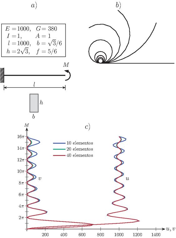
Figure 5 Cantilever beam under pure bending: (a) geometric and mechanical properties, (b) deformed configurations at 1, 2, 3, 4, and 5 full revolutions, and (c) equilibrium paths for different mesh refinements.

Figure 5(a) details the geometric and mechanical properties. The beam was discretized into meshes of 10, 20 and 40 elements; more refined meshes are necessary to accurately represent the smaller radii of subsequent revolutions. A total rotation of $2\pi /10$ was imposed per load step at the free end, requiring 10 steps to complete one full revolution.

In this simulation, eight full revolutions (2880 degrees of rotation) were completed over 80 load steps. At this stage, the radius reaches a value of $1000/16\pi \approx 19.89$. Figure 5(b) illustrates the deformed configurations at selected stages: 1, 2, 3, 4 and 5 complete revolutions, corresponding to end rotations of $2\pi$, $4\pi$, $6\pi$, $8\pi$ and $10\pi$ radians, respectively. These visualizations clearly demonstrate the beam progressively curling into tighter spirals as the applied moment increases. The ability of the formulation to track these extreme deformations without numerical divergence validates the robustness of the modulo function strategy (Eq. 8) for handling large rigid-body rotations. It should be noted that the radius of curvature decreases linearly with the number of revolutions, as expected from the theoretical relationship $r=l/2\pi n$, where $n$ is the number of complete circles. These deformed configurations were obtained with 40 elements. Note that with 40 elements, it is not possible to accurately represent eight circles because the element length ($1000/40=25$) exceeds the final radius ($1000/(8\times 2\pi )=19.89$). Accurately capturing eight revolutions requires a discretization of at least 51 elements. Figure 5(c) plots the horizontal and vertical displacements of the free end for various meshes up to eight full revolutions. As the mesh is refined, the precision improves significantly across successive revolutions. For the 10 element mesh, the equilibrium path was obtained with an average of 5.68 iterations; the 20 element mesh averaged 5.04, and the 40 element mesh averaged 6 iterations.

6.2 Lee’s Frame

As shown in Figure 6(a), Lee’s frame consists of a beam and a column joined at a right angle. One end is pinned (fixed in $x$ and $y$), while the other is constrained horizontally but free to displace along the $y$-axis. The frame was discretized using 20 elements for each of the EB, TI, and SAB models. The load conditions, as well as the geometric and mechanical properties are detailed in Figure 6(a).

Figure 6(b) illustrates the vertical displacements $v_1$ and $v_2$ throughout the loading process. The equilibrium trajectories are largely coincident for all three models, except near the limit points PL2, PL4, and PL5. These results were compared with the trajectories reported by Fujii et al. [11], who used a 10 element mesh. While there is strong general agreement, the 20 element mesh used here captures complex looping behavior at limit points PL2, PL3, and PL4 that the coarser mesh misses.

Figure 6(c) presents selected deformed configurations corresponding to critical points along the equilibrium path. At limit point PL2, the frame exhibits a pronounced snap-through behavior with significant lateral deflection. The configurations at PL3 and PL4 reveal the complex looping behavior, where the structure traverses multiple equilibrium states at similar load levels but vastly different displacement patterns. These visualizations underscore the severe geometric nonlinearity of this problem and illustrate why capturing such behavior requires both refined discretization and robust solution algorithms. The deformed shapes also confirm that all three element formulations (EB, TI, SAB) produce qualitatively consistent deformation patterns, with quantitative differences emerging only in the precise load levels at limit points.

To capture this highly nonlinear response characterized by multiple limit points, turning points, and snap-back loops, the arc-length method with a cylindrical constraint was employed. An initial arc-length of 12.5 was used for all models. For the EB element, 285 load steps were required, including 43 automatic step-size reductions due to divergence, with an average of 4.43 iterations. The SAB element required 300 steps with 55 cuts and an average of 4.41 iterations. The TI element required 350 steps with 78 cuts and an average of 4.65 iterations.

Figure 7 provides a detailed mesh convergence study comparing 10-element and 20-element discretizations for each beam theory. For the TI element (Figure 7(a)), the 10-element mesh successfully captures the initial equilibrium path and the first two limit points but fails to resolve the complex looping behavior at PL3, and PL4, eventually leading to convergence difficulties. This sensitivity to mesh refinement is attributable to the linear interpolation functions employed in the TI formulation, which limit its ability to represent sharp curvature gradients accurately. The EB element (Figure 7(b)) demonstrates improved performance with the coarser mesh, showing good agreement in the linear regime and moderate agreement near limit points, though the detailed loop structure is not fully captured until the mesh is refined to 20 elements. In contrast, the SAB element (Figure 7(c)) exhibits remarkable mesh-to-mesh consistency, with the 10-element and 20-element trajectories nearly coincident throughout the entire response, including all complex loops. This superior convergence characteristic stems from the SAB element’s explicit treatment of axial-bending coupling (Eq. 49), which accurately represents the membrane-bending interaction that dominates the structural behavior in this problem. These convergence studies confirm that while all three formulations are theoretically sound within the unified corotational framework, the SAB element offers the most efficient path to accurate solutions for problems involving significant geometric nonlinearity.

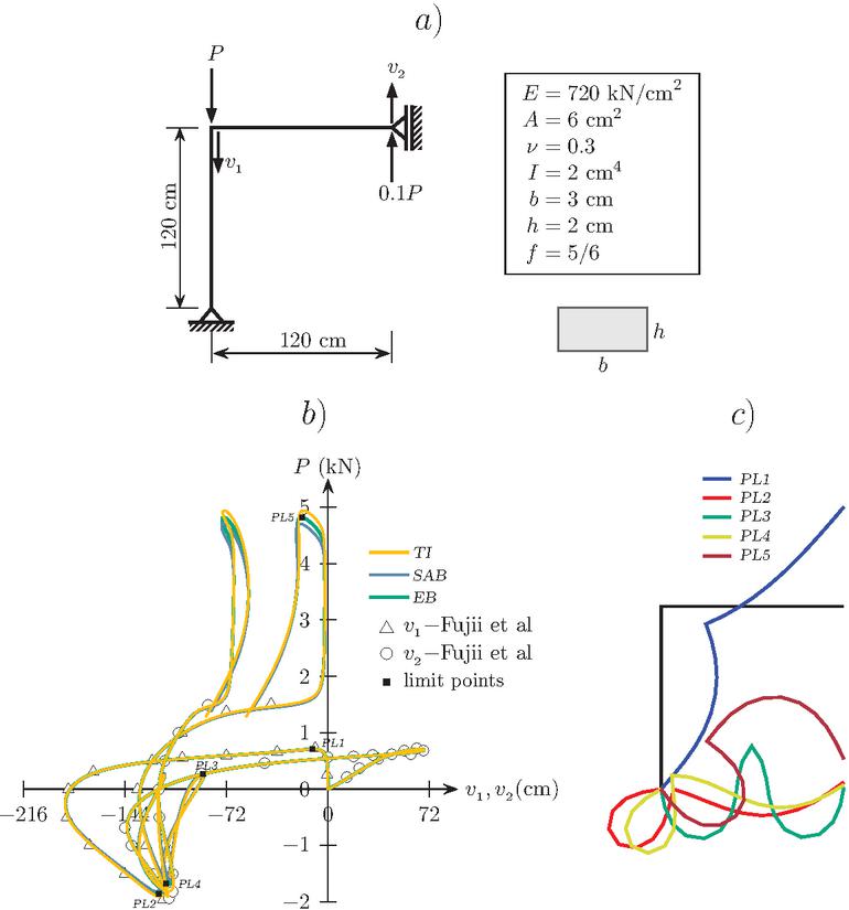
Figure 6 Lee’s frame: (a) geometric and mechanical properties, (b) primary equilibrium paths for EB, TI, and SAB elements compared with reference data, and (c) deformed configurations at selected limit points.

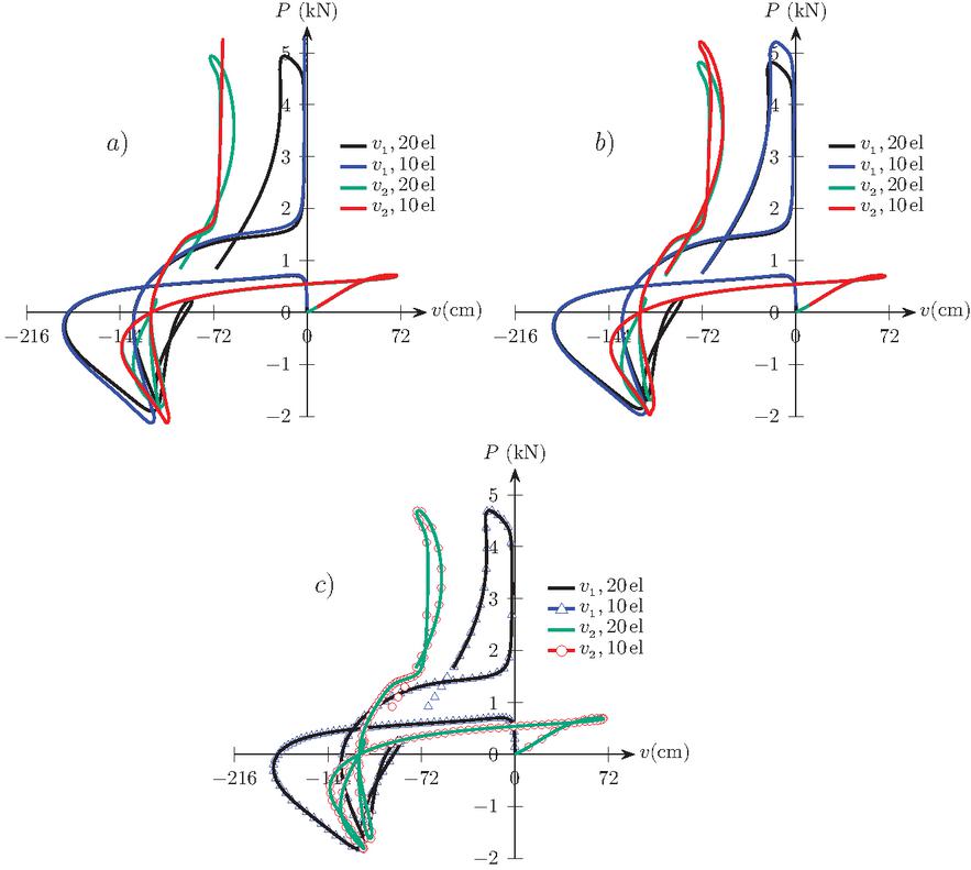
Figure 7 Primary paths comparison for 10 and 20 element meshes: (a) Timoshenko, (b) Euler-Bernoulli, and (c) Shallow arch Euler-Bernoulli elements.

6.3 Hinged Shallow Arch

Figure 8(a) illustrates a hinged circular shallow arch subjected to a uniformly distributed load $q$ over half of its span. The geometric and mechanical properties are provided in the figure. The arch was discretized using 20 elements for each of the EB, TI, and SAB models.

Figure 8(b) presents the normalized equilibrium paths ($\frac{q{r}^3}{EI}$ vs. $\frac{v}{r}$) obtained with the three element types. No significant discrepancies are observed between the trajectories, except in the proximity of the limit points PL2, PL3, and PL4. Table 1 compares the normalized load values at limit points PL1, PL2, and PL3 with the results reported by Xu and Mirmiran [12], who utilized a corotational formulation with an element incorporating nonlinear Green-Lagrange strain terms.

Figure 8(c) displays deformed configurations at representative stages of the loading process. The initial configuration shows the arch in its undeformed state. As loading progresses, the arch undergoes a first snap-through at limit point PL1, transitioning to an inverted configuration. Subsequent loading leads to complex looping behavior (PL2, PL3) where the structure oscillates between different equilibrium states. The final configuration at PL4 illustrates the extreme deformation capacity tracked by the formulation. These visualizations confirm that the shallow arch problem involves not only significant rigid-body motion but also substantial local deformation, justifying the importance of the axial-bending coupling incorporated in the SAB element.

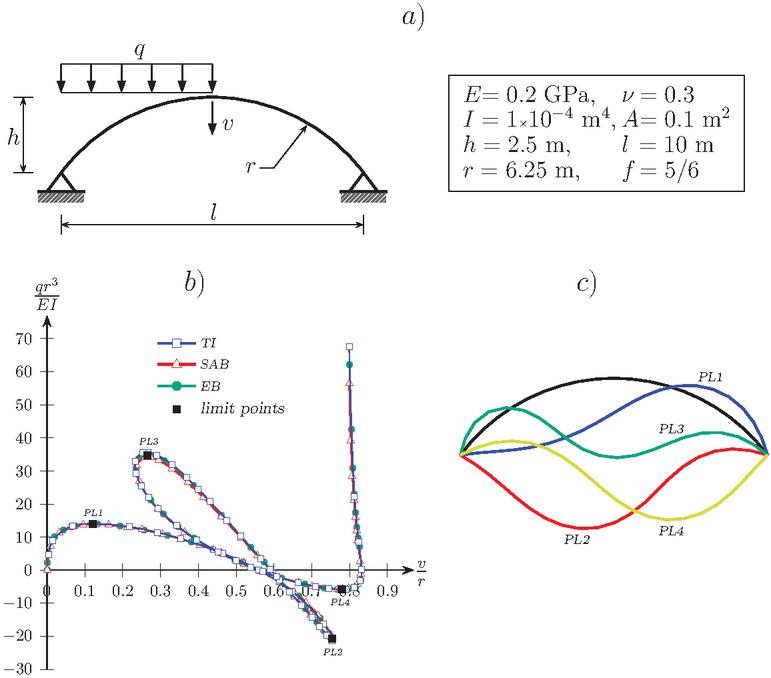
Figure 8 Hinged shallow arch: (a) geometric and mechanical properties, (b) primary equilibrium paths for EB, TI, and SAB, and (c) deformed configurations at limit points.

For the EB element, the maximum discrepancy was 3.1% at PL2. The SAB element demonstrated the highest accuracy, with a maximum difference of only 0.8% at PL2. The TI element exhibited a maximum difference of 5.92% at PL2; this higher discrepancy is attributed to the use of linear interpolation functions.

The equilibrium paths were obtained using a variable displacement control method with an initial arc-length of 0.1 for all three element types. The EB model required 177 load steps with 12 automatic step reductions and an average of 4.18 iterations. The SAB model required 173 steps with 10 reductions and an average of 4.20 iterations. The TI model required 173 steps with 9 reductions and an average of 4.22 iterations. As shown in Figure 8(b), the structural response is highly nonlinear, featuring multiple limit points, turning points, and a distinct loop.

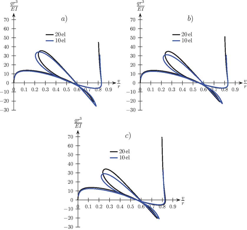
Figure 9 Mesh convergence study for the hinged shallow arch-comparison of 10-element and 20-element discretizations: (a) Timoshenko element, (b) Euler-Bernoulli element, and (c) shallow arch Euler-Bernoulli element.

Table 1 Values of the load $\frac{q{r}^3}{EI}$ at limit points

	PL1	PL2	PL3
Xu and Mirmiran	13.77	-20.09	33.99
EB	13.92	-20.71	34.86
diff. (%)	1.09	3.09	2.56
SAB	13.83	-20.25	34.17
diff. (%)	0.44	0.8	0.53
TI	14.02	-21.28	35.62
diff. (%)	1.82	5.92	4.8

Figure 9 presents a comprehensive mesh convergence study comparing 10-element and 20-element discretizations for each beam formulation. This comparison is essential for initially curved structures, as the element chord may not align with the structural tangent, requiring sufficient discretization to accurately represent the curved geometry and the distributed loading.

For the TI element (Figure 9(a)), noticeable differences exist between the two meshes, particularly in the looping regions near limit points PL2 and PL3. The 10-element mesh underestimates the load capacity at these critical points, and the loop geometry differs substantially from the refined mesh. This mesh sensitivity reflects the TI element’s reliance on linear interpolation, which struggles to capture the rapid curvature variations characteristic of snap-through behavior in shallow arches.

The EB element (Figure 9(b)) demonstrates improved mesh-to-mesh agreement compared to the TI formulation, owing to its cubic shape functions for transverse displacement. However, subtle differences persist near the limit points, indicating that even with higher-order interpolation, the coupling between axial and bending effects in shallow arches requires careful discretization when using conventional beam theories that treat these effects independently.

Most significantly, the SAB element (Figure 9(c)) exhibits exceptional convergence characteristics, with the 10-element and 20-element trajectories virtually indistinguishable throughout the entire equilibrium path, including all limit points and loops. This superior performance is directly attributable to the SAB formulation’s explicit incorporation of axial-bending coupling (Eq. 49), which accurately captures the physical behavior of shallow arches where membrane action significantly influences bending response. The axial strain in Eq. 49 includes quadratic terms in the rotational degrees of freedom (${\overline{\theta }}_1^{{}^2}$, ${\overline{\theta }}_2^{{}^2}$, ${\overline{\theta }}_1{\overline{\theta }}_2$), enabling the element to represent the geometric nonlinearity more accurately with coarser meshes.

These convergence studies confirm that while all three formulations converge to similar solutions with sufficient mesh refinement, the SAB element achieves engineering accuracy with significantly fewer degrees of freedom, making it the most efficient choice for shallow arch analysis within the unified corotational framework.

6.4 Hinged Semicircular Arch

Figure 10(a) depicts a hinged semicircular arch subjected to a point load $P$ eccentric with respect to its vertex. The geometric and mechanical properties are detailed in the figure. The arch was discretized using 50 elements for the EB, TI, and SAB models.

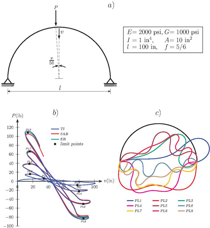
Figure 10 Hinged semicircular arch: (a) geometric and mechanical properties, (b) primary equilibrium paths for EB, TI, and SAB elements, and (c) deformed configurations at selected limit points.

Figure 10(b) shows the load $P$ versus the vertex vertical displacement $v$ for the three beam models. The equilibrium trajectories coincide closely during the initial loading stages; however, noticeable discrepancies emerge in the vicinity of the higher-order limit points PL6, PL7, PL8, and PL9.

Figure 10(c) presents deformed configurations at selected stages throughout the loading history. The sequence illustrates the progressive evolution from the initial circular geometry through multiple snap-through events (PL1 through PL9). The extreme deformations exhibited in the later stages-particularly beyond PL6-demonstrate the formulation’s capability to track highly nonlinear equilibrium paths involving substantial changes in structural geometry. These configurations also reveal that the arch experiences not only bending deformation but also significant axial shortening and elongation, further justifying the importance of the membrane-bending coupling in the SAB formulation. The visual comparison between configurations at different limit points clarifies why conventional beam theories that neglect this coupling may encounter accuracy limitations in such extreme deformation regimes.

Table 2 compares the load values $P$ at nine distinct limit points with the reference values provided by Yang and Kuo [13], who employed an updated Lagrangian formulation with a beam element including nonlinear Green-Lagrange strain terms and a 26 element mesh. For the EB element, the maximum discrepancy was 3.82% at limit point PL9. The SAB element proved the most accurate, with a maximum difference of only 1.76% at limit point PL8. The TI element exhibited the largest deviation, reaching 6.88% at limit point PL9. While the differences were negligible at the first four limit points (PL1 through PL4), the geometric nonlinearities at the later stages (PL6 through PL9) highlight the superior performance of the refined SAB kinematics.

The equilibrium paths were computed using the variable displacement control method, with an initial arc-length of 2.2 for all models. The EB model required 859 load steps with 91 automatic cuts due to divergence and an average of 4.23 iterations. The SAB model required 820 steps with 93 cuts and an average of 4.25 iterations. The TI model required 859 steps with 89 cuts and an average of 4.22 iterations. As shown in Figure 10(b), the arch response is characterized by extreme nonlinearity, including numerous limit points, turning points, and complex loops.

Table 2 Values of the load $P$ at limit points (lb)

	PL1	PL2	PL3	PL4	PL5
Yang and Kuo	5.813	$-$8.498	16.149	$-$22.162	38.566
EB	5.811	$-$8.495	16.204	$-$22.086	38.932
diff. (%)	0.03	0.04	0.34	0.34	0.95
SAB	5.802	$-$8.464	16.108	$-$21.912	38.453
diff. (%)	0.19	0.40	0.25	1.13	0.29
TI	5.816	$-$8.518	16.278	$-$22.24	39.328
diff. (%)	0.05	0.24	0.80	0.35	1.98
	PL6	PL7	PL8	PL9
Yang and Kuo	$-$49.896	64.875	$-$82.420	104.611
EB	$-$50.206	66.786	$-$83.138	108.61
diff. (%)	0.62	2.95	0.87	3.82
SAB	$-$49.394	65.274	$-$80.967	104.99
	1.00	0.62	1.76	0.36
TI	$-$50.909	68.081	$-$85.055	111.81
diff. (%)	2.03	4.94	3.20	6.88

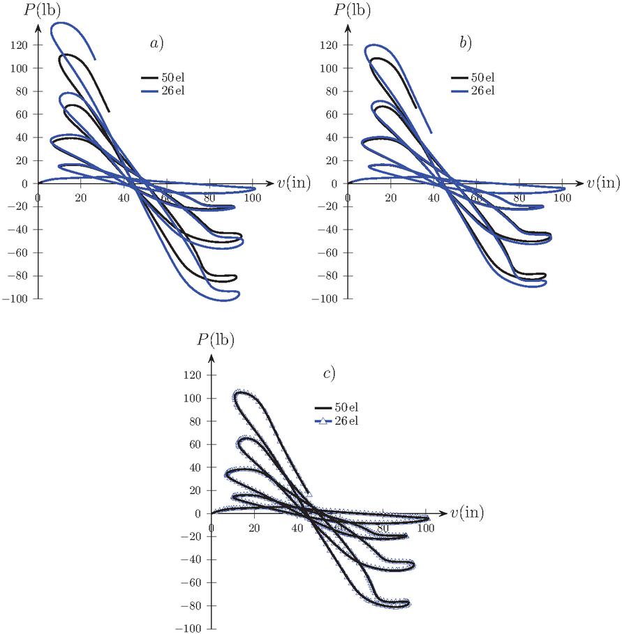
Figure 11 Mesh convergence study for the hinged semicircular arch-comparison of 26-element and 50-element discretizations: (a) Timoshenko element, (b) Euler-Bernoulli element, and (c) shallow arch Euler-Bernoulli element.

Figure 11 provides a detailed mesh convergence analysis comparing 26-element and 50-element discretizations for the semicircular arch problem. Given the extreme geometric nonlinearity exhibited by this structure-evidenced by the nine distinct limit points and multiple complex loops-this convergence study is critical for assessing the reliability of each formulation.

For the TI element (Figure 11(a)), the two meshes show reasonable agreement through the first two loops (limit points PL1 through PL4), where deformations remain moderate. However, as the loading progresses and geometric nonlinearity intensifies beyond PL5, significant discrepancies emerge. The 26-element mesh begins to diverge from the refined solution, failing to accurately capture the load levels and displacement amplitudes at the higher-order limit points (PL6 through PL9). In some regions, the coarser mesh even fails to converge, necessitating excessive load step reductions. This progressive deterioration in accuracy reflects the fundamental limitation of linear interpolation functions when representing the severe curvature variations that develop in the later stages of loading.

The EB element (Figure 11(b)) demonstrates improved behavior relative to the TI formulation, with both meshes tracking each other more consistently through the intermediate loops. Nevertheless, noticeable differences persist, particularly in the precise load values at limit points PL7, PL8, and PL9, where discrepancies of 2-4% are observed (Table 2). While cubic shape functions provide superior curvature representation, the EB formulation’s treatment of axial and bending effects as uncoupled phenomena introduces cumulative errors in problems where these effects interact strongly, as is the case in deeply deformed arches.

Most remarkably, the SAB element (Figure 11(c)) exhibits near-perfect mesh-to-mesh agreement throughout the entire equilibrium path, including all nine limit points and the intricate looping behavior. The 26-element and 50-element trajectories are virtually indistinguishable, even in the extreme deformation regime beyond PL6 where the other formulations show substantial mesh sensitivity. This exceptional convergence characteristic directly demonstrates the effectiveness of the axial-bending coupling incorporated in the SAB formulation (Eqs. 49 and 53). By explicitly accounting for the quadratic dependence of axial strain on rotational degrees of freedom, the SAB element captures the essential physics of the problem with remarkable efficiency.

Quantitatively, Table 2 confirms these observations: the maximum discrepancy between SAB predictions and reference solutions is only 1.76% (at PL8), compared to 3.82% for EB and 6.88% for TI. More significantly, the SAB results show minimal variation between the 26-element and 50-element meshes, indicating that the coarser discretization already provides engineering accuracy. This convergence behavior suggests that for highly nonlinear arch problems, the SAB element can achieve reliable solutions with substantially fewer degrees of freedom than conventional beam formulations, offering significant computational efficiency advantages for large-scale structural analysis.

In summary, the mesh convergence studies for both the shallow arch (Figure 9) and the semicircular arch (Figure 11) consistently demonstrate that the SAB element’s superior kinematic formulation translates directly into superior numerical performance, particularly in problems involving extreme geometric nonlinearity where membrane-bending coupling effects dominate structural response.

7 Conclusions

This paper presented a unified corotational framework applied to three distinct 2D beam kinematics: Euler-Bernoulli (EB), Timoshenko (TI), and shallow arch Euler-Bernoulli (SAB). The numerical examples demonstrate that the proposed formulations exhibit excellent performance in the geometrically nonlinear analysis of beams, frames, and arches. For problems involving infinitesimal strains, the equilibrium trajectories across all three models are practically identical and show strong agreement with established benchmarks in the literature. As strain magnitudes increase, the refined kinematics of the SAB element offer superior precision, particularly in capturing complex post-buckling behavior and looping trajectories.

Several key conclusions and contributions can be drawn from this work:

1. Numerical Robustness: The implementation of the modulo function strategy effectively overcomes the traditional singularity problems associated with large rigid body rotations. The examples demonstrate that the formulation remains stable even through multiple full revolutions (rotations exceeding $2\pi$), a critical requirement for highly flexible structures.

2. Kinematic Decoupling: A significant advantage of this corotational approach is the explicit decoupling of local deformational effects from global rigid body motion. This modularity allows for the integration of standard linear finite element libraries into a high-performance nonlinear engine through straightforward algebraic operations.

3. Theoretical Unification: The primary theoretical contribution of this research is the rigorous unification of the corotational formulations proposed by Crisfield [1] and Krenk [2]. Through systematic algebraic derivation, we have demonstrated that despite their fundamentally different kinematic approaches-projection-based versus equilibrium-based-these formulations yield algebraically identical tangent stiffness matrices in global coordinates. This identity holds for arbitrary magnitudes of rigid-body rotations and deformations, establishing that the two frameworks are not merely similar but mathematically equivalent. The analytical proof of equivalence ensures that numerical results obtained using our implementation are indistinguishable from those from either Crisfield’s or Krenk’s original formulations, eliminating any ambiguity regarding the choice between these frameworks. While the primary contribution is theoretical, the unified framework offers practical advantages in terms of code modularity, pedagogical clarity, and the seamless integration of diverse beam theories within a single computational platform. By deriving a consistent geometric stiffness matrix that is independent of the local beam theory, we provide a versatile framework where the same global operator can be associated with various local tangent stiffness matrices (EB, TI, or SAB) without loss of objectivity.

4. Computational Efficiency and Convergence Characteristics: The formulation achieves high precision with relatively coarse meshes, particularly when employing the SAB element. Comprehensive mesh convergence studies presented for the shallow arch (Section 6.3, Figure 9) and semicircular arch (Section 6.4, Figure 11) demonstrate that:

• The Timoshenko element, while correctly capturing shear flexibility, exhibits significant mesh sensitivity in highly nonlinear regimes due to its linear interpolation functions. Coarse meshes may fail to resolve complex looping behavior near limit points.

• The Euler-Bernoulli element shows improved convergence characteristics owing to its cubic shape functions, though subtle discrepancies persist in problems where axial-bending coupling is significant.

• The shallow arch Euler-Bernoulli element demonstrates exceptional convergence properties, with coarse meshes (10-26 elements) producing results nearly indistinguishable from refined meshes (26-50 elements). This superior performance stems from the explicit treatment of axial-bending coupling (Eqs. 49, 53), which accurately represents the dominant physical mechanisms in geometrically nonlinear arch and frame problems.

These convergence characteristics indicate that the choice of local beam theory (${\text{K}}_d$) significantly influences computational efficiency, while the unified corotational framework ensures consistent and objective treatment of large rigid-body motions across all formulations. The Timoshenko element was shown to be free of shear locking through the single-point Gauss integration strategy employed in Eq. (44), while the SAB element effectively mitigated membrane locking through the averaged axial strain formulation in Eq. (48), ensuring reliable convergence in severely nonlinear equilibrium paths involving limit points and snap-backs.

5. Extension to Three-Dimensional Kinematics While the present work focuses exclusively on planar beam elements, the unified corotational framework is conceptually extensible to three-dimensional kinematics. The fundamental principle of decomposing total motion into rigid-body and deformational components, along with the theoretical equivalence between projection-based (Crisfield) and equilibrium-based (Krenk) approaches, remains valid in 3D. However, such an extension introduces several additional complexities that warrant dedicated investigation:

• Finite rotation parametrization: Three-dimensional rotations are inherently non-commutative, requiring careful selection of rotation parameters (e.g., Euler angles, Rodrigues parameters, quaternions, or rotation vectors) to avoid singularities while ensuring objectivity and path-independence of the formulation.

• Torsion-bending coupling: In 3D beam elements, particularly those with thin-walled or open cross-sections, significant coupling exists between torsional and bending deformations (warping effects). The local elastic stiffness matrix ${\text{K}}_d$ must account for these interactions, substantially increasing algebraic complexity.

• Generalization of the modulo function strategy: The numerical approach developed in Eq. (8) for handling large rotations about a single axis must be extended to accommodate simultaneous large rotations about multiple axes, ensuring continuity of all rotational variables during multi-revolution motions.

• Transformation matrix complexity: The transformation matrix B (Eq. 11) generalizes to higher dimensions, incorporating three rotational degrees of freedom per node and requiring careful derivation to maintain consistency between local and global kinematic descriptions.

Despite these challenges, the modular structure of the unified framework facilitates such extensions by allowing the local elastic stiffness matrix to be replaced with 3D counterparts while maintaining the same fundamental corotational machinery. The 2D unification presented here establishes an essential theoretical foundation, clarifying fundamental relationships and numerical strategies before tackling the additional complexities of three-dimensional kinematics. Future research will address these aspects, building upon the clarified theoretical foundation established herein for the planar case.

In summary, the unified corotational formulation described herein provides a robust, efficient, and mathematically transparent tool for the large-displacement analysis of planar structures. The theoretical synthesis of the Crisfield and Krenk frameworks eliminates long-standing ambiguities in the literature while establishing a modular computational platform that facilitates the integration of diverse beam theories. The comprehensive numerical validation demonstrates that the formulation handles extreme geometric nonlinearities with exceptional stability and accuracy, making it well-suited for analyzing highly flexible structures undergoing complex deformation patterns. Future extensions to three-dimensional kinematics, material nonlinearity, and dynamic analysis represent natural progressions of this research, leveraging the clarified theoretical foundation and computational architecture established in the present work.

Conflict of Interest Statement

The authors declare that they have no known competing financial interests or personal relationships that could have appeared to influence the work reported in this paper.

The Funding Statament

The authors declare that this article was not funded by government or private agencies.

References

[1] Crisfield M.A. Non-linear finite element analysis of solids and structures, Volume 1: Essentials. John Wiley & Sons, 1991.

[2] Krenk S. Non-linear modeling and analysis of solids and structures. Cambridge University Press, 2009.

[3] Krenk S. A general format for curved and non-homogeneus beam elements. Computers & Structures, 50 (4), 449–454, 1994.

[4] Krenk S., Vissing-Jorgensen C. and Thesbjerg L. Efficient collapse analysis techniques for framed structures. Computers & Structures, 72, 481–496, 1999.

[5] Silva W. T. M., Cunha A. A. and Gutiérrez M. P. D. Nonlinear analysis of plane frames using a co-rotating Timoshenko beam element. Journal of Building Technology, 6 (2), 1–16, 2024.

[6] Tang Y. Q., Du E. F., Wang J. Q. and Qi J. N. A co-rotational curved beam element for geometrically nonlinear analysis of framed structures. Structures, 27, 1202–1208, 2020.

[7] Heng P., Alhasawi A., Battini J. M. and Hjiaj M. Co-rotating rigid beam with generalized plastic hinges for the nonlinear dynamic analysis of planar framed structures subjected to impact loading. Finite Elements in Analysis and Design, 157, 38–49, 2019.

[8] Doan-Ngoc T. N., Dang X. L., Chu Q. T., Balling R. J. and Ngo-Huu C. Second-order plastic-hinge analysis of planar steel frames using corotational beam-column element. Journal of Constructional Steel Research, 121, 413–426, 2016.

[9] Kien N. D. A Timoshenko beam element for large displacement analysis of planar beams and frames. International Journal of Structural Stability and Dynamics, 12 (6), 1–9, 2012.

[10] Metcalf M., Reid J. and Cohen M. Modern Fortran explained. Eighth edition, Oxford University Press, 2018.

[11] Fujii F., Choong K. K and Gong S. X. Variable displacement control to overcome turning points of nonlinear elastic frames. Computers & Structures, 44 (1–2), 133–136, 1992.

[12] Xu Z. and Mirmiran A. Looping behavior of arches using corotational finite element. Computers & Structures, 62 (6), 1059–1071, 1997.

[13] Yang Y. B. and Kuo S. R. Theory & analysis of nonlinear framed strucutures. Prentice Hall, 1994.

Biographies

William T. M. Silva was born in 1959. Full professor, University of Brasília, Brazil. Ph.D. in 1996 at the Polytechnic University of Catalonia, Spain. Interest fields are nonlinear analysis of solids and structures.

Éder R. L. Nascimento was born in 1990. Graduated in 2013 from University Federal of Rio Grande do Norte, Brazil. M.Sc. in 2021 at the University of Brasília, Brazil. Interest fields are computational mechanics, nonlinear structural analysis, structural durability and structural reliability.

Sebastião S. da Silva was born in 1983. Graduated in 2008 from University Federal of Campina Grande, Brazil. Ph.D. in 2019 at the University of Brasília, Brazil. Interest fields are computational mechanics and nonlinear analysis of structures.

A. Portela was born in 1951. Full professor, University of Brasília, Brazil. Ph.D. in 1992 at the Wessex Institute of Technology, United Kingdom. Interest fields are computational mechanics and boundary element method.

European Journal of Computational Mechanics, Vol. 35_1, 1–36
doi: 10.13052/ejcm2642-2085.3461
© 2026 River Publishers