A 6-Parameter Triangular Flat Shell Element for Nonlinear Analysis

Mohammad Rezaiee-Pajand^∗, Amir R. Masoodi and E. Arabi

Department of Civil Engineering, Ferdowsi University of Mashhad, Mashhad, Iran
Email: rezaiee@um.ac.ir
^*Corresponding Author

Received 01 February 2019; Accepted 05 August 2019;
Publication 06 September 2019

Abstract

In this paper, an improved flat triangular shell element is proposed. This element has three nodes, and in each node, six degrees of freedom are considered. Since there are three rotational degrees of freedom at each node, the drilling effect can be incorporated in authors’ formulation. A new procedure is also suggested for updating the director vectors about which the rotational degrees of freedom are defined. In order to study large displacements and rotations, Total Lagrangian principles are employed. In addition, updating the rotational degrees of freedom is implemented using enriched updated director vectors, which are formulated based on the finite rotation method. On the other hand, small strains are considered in this formulation. By utilizing MITC method, shear and membrane locking is mitigated from new element. To examine the performance, the element passes three basic tests, including isotropy, and patch test. Moreover, a convergence study is also implemented to show the elemental behavior. Several popular benchmarks are considered to illustrate the accuracy and capability of the suggested element in geometrically nonlinear analyses.

Keywords: Flat triangular shell element, Total Lagrangian formulation, drilling, MITC approach, geometrically nonlinear analysis

Nomenclature

$t_i$	The thickness of node i
$\{{}_{0}B\}$	The linear strain–displacement matrix
$e_{ij}$	Linear part of strain tensor
$e_1,e_2,e_3$	The unit vector in global Cartesian system
$N_i\left(r,s,t\right)$	The two dimensional interpolation functions
$\{{}_{0}N\}$	The nonlinear strain–displacement matrix
$r,s,\zeta$	The convected coordinates
$\left\{u\right\}$	The nodal displacement vector in global Cartesian system
$U$	Vector of incremental nodal displacements
$u,v,w$	The nodal displacements
$u_l,v_l,w_l$	The linear part of nodal displacement
$u_q,v_q,w_q$	The quadratic part of nodal displacement
$V_1^i,V_2^i$	The unit vectors orthogonal to $V_n^i$ and to each other
${\left\{V_n\right\}}^i$	The director vector of node i
$\left\{x\right\}$	The position vector of node
${\alpha }_i,{\beta }_i$	The rotation of $V_n^i$ about $V_1^i$, $V_2^i$
${\epsilon }_{ij}$	Green-Lagrange strain tensor
${\eta }_{ij}$	Nonlinear part of strain tensor

1 Introduction

Nonlinear analyses are employed to predict the real behavior of structures. On the other hand, geometrically nonlinear analysis is one of the most important parts of these analyses. One of the structures with this complex behavior is the shell structures, which play a significant role in the field of civil engineering. Based on this fact, many researchers have been attracted to study the geometrically nonlinear behavior of different types of shells. They proposed diverse shell elements and employed various types of altered formulations to predict the behavior of shell structures more accurate and reliable. The main goal can be achieved by suggesting an element with lower degrees of freedom and higher accuracy. Once drilling degree of freedom can improve the linear and nonlinear behavior of shell elements, this subject can be taken into account in details. Based on the obtained results of pervious investigators, it can be concluded that drilling degree of freedom can improve the performance of the shell element, especially in the geometrically nonlinear analysis. In addition, it can be easily utilized for connecting to space beam elements. This topic can be investigated with more details.

Degenerated shell elements are sets of the most applicable tools, which have attracted the courtesy of more researchers in the linear and nonlinear analyses. In 1970, Ahmad et al. proposed this approach, for the first time, to analyze thin and thick curved shell structures [1]. After that, this method was developed by many other researchers using different types of shell element [2–7]. To improve this approach, some studies were performed by using strain interpolation. Among them, Bathe and Dvorkin employed the formulation of general shell elements. They used Mixed Interpolation of Tensorial Components (MITC) to avoid shear and membrane locking in their proposed element [8]. Moreover, some more studies were developed to use this technique [2, 9–17].

Recently, the MITC method was employed to formulate the triangular shell elements. A three-node triangular shell element was also formulated by Lee et al. [18]. In 2009, Kim and Bathe employed a six-node triangular shell element for the linear analysis of shell structures [19]. In addition, an improvement was considered for the three-node shell element using the Hellinger–Reissner principle by Lee et al. [20]. In another research, a 3-node MITC shell element, which had been developed before, was enriched by interpolation covers using new tying points [21]. In 2014, a four-node triangular shell element entitled (MITC3 $+$) was proposed by Lee et al. They used a bubble function for the middle node of element. The middle node of element has two rotational degrees of freedom [22]. Furthermore, the use of MITC3 $+$ in the geometrically nonlinear analysis of shell structures was incorporated by Jeon et al. In addition, to consider large deflection, Total Lagrangian formulation was employed. They also proved that the proposed element can be utilized for large rotation problems [23]. A recently published research which was about proposing a six-node triangular shell element was performed by Rezaiee-pajand et al. They used MITC method to prevent locking phenomena, especially in nonlinear analysis [24]. Besides, application of this element on thermo-mechanical analysis of shells structures in thermal environments was investigated by Masoodi and Arabi. They used finite element procedure to solve complicated shell problems under thermo-mechanical loads [25]. It is observed that many researches were implemented about MITC approach to improve shell elements for linear and especially geometrically nonlinear analysis of shell structures. However, there is no drilling degree of freedom in this formulation. Hence, this limitation can be improved and eliminated.

A topic which has attracted the attention of researchers is to include drilling degree of freedom in their shell elements. In the past decades, plane elements with drilling degree of freedom were widely developed to use in the linear and nonlinear analysis of plane structures [26–29]. Gradually, this subject was considered in shell elements. In 1991, a flat triangular and quadrilateral shell element using discrete Kirchhoff plate bending elements and the membrane elements with drilling degrees of freedom [30]. It was proven that the locking phenomena in this type of formulation have an effective role. Another research was also presented by Gruttmann et al. to analyze the structures nonlinearly using a quadrilateral shell element with drilling degree of freedom [31]. Some other investigations developed assumed-stress hybrid shell elements enriched by drilling degree of freedom for linear and nonlinear static and dynamic problems [32–34]. In 2014, a flat shell element with drilling degree of freedom was formulated by Shin and Lee. They used natural deviatoric strain method to solve the doubly-curved shell structures [35].

Development of Moreover, nonlinear static analysis of plate structures was investigated by Nguyen-Van et al. using MISQ26 element with drilling degree of freedom made of functionally graded materials [36]. To use in shape sensing and structural health monitoring, a quadrilateral inverse-shell element with degree of freedom was presented by Kefal et al. [37]. Recently, a new quadrilateral shell element was proposed to use in the geometrically nonlinear analysis by Tang et al. They considered and investigated drilling, shear and warping effects on the obtained results of linear and nonlinear analyses [38]. Another study which is performed on developing triangular shell elements including drilling degree of freedom was presented recently [39, 40].

Accordingly, many studies were implemented on the proposing shell elements and employing in nonlinear analysis, especially geometrically ones. Although, these investigations reached almost near exact responses, there are still ambiguous points, which are required to be clarified. One of the important topics which were recently studied by other researches is incorporating drilling degree of freedom into formulation of shell elements. The main objective of this paper is taking enriched shell element with drilling into account. This subject has essential effects on the obtained responses, especially problems in which large rotations play an important role. In order to perform geometrically nonlinear analysis, a new improved three-node triangular shell element is proposed based on the continuum model of shells using the finite-element method. It is worth mentioning that six degrees of freedom, including, three transitional and three rotational are assigned to each elemental node. In other words, drilling degrees of freedom are considered in this formulation. A new procedure is also suggested for updating the director vectors related to the rotational degrees of freedom. This proposed method enables the authors to incorporate drilling degree of freedom in MITC shell element and improve its bending behavior, especially in the large rotation problems. In addition, Total Lagrangian principles are employed for geometrically nonlinear analysis. It should be added that large deflections and rotations are considered with small strain. To release the shear and membrane locking, MITC approach is used. Several benchmark problems are also solved by using the suggested element. Although this formulation enables the analyzer to consider loading with drilling component, the main purpose of this research is studying the effect of the proposed procedure on the obtained responses of geometric nonlinear analysis by solving well-known benchmarks. Findings illustrate that authors’ scheme has high accuracy and capability in the nonlinear analysis of shell structures.

2 Linear Kinematical Three-node Element

The kinematic and geometric basics of the three-node element are described in this section. Figure 1 illustrates the proposed element and the origin of the reference system (r, s, $\zeta$). The director vectors, which are defined at each node, are also depicted in Figure 1.

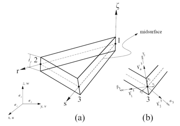
Figure 1 Geometry of triangular shell element (a) 3-node element (b) director vectors.

The new element is considered to have 6 degrees of freedom per shell node: Three transitions and three rotations. To develop formulation, the shell geometry at time 0 is interpolated as follows:

$$\begin{array}{r}{}^0\left\{\begin{array}{c}x(r,s,\mathrm{\zeta <!--\; \zeta \; -->})\\ y(r,s,\mathrm{\zeta <!--\; \zeta \; -->})\\ z(r,s,\mathrm{\zeta <!--\; \zeta \; -->})\end{array}\right\}=\underset{i=1}{\overset{3}{\sum <!--\; \sum \; -->}}{N}^i(r,s{)}^0{\left\{\begin{array}{c}x(r,s,\mathrm{\zeta <!--\; \zeta \; -->})\\ y(r,s,\mathrm{\zeta <!--\; \zeta \; -->})\\ z(r,s,\mathrm{\zeta <!--\; \zeta \; -->})\end{array}\right\}}_M^i+\frac{\mathrm{\zeta <!--\; \zeta \; -->}}{2}\underset{i=1}{\overset{3}{\sum <!--\; \sum \; -->}}{N}^i(r,s){}^0{t}^i{}^0{\left\{\begin{array}{c}{V}_n^x\\ V_n^y\\ V_n^z\end{array}\right\}}^i\end{array}$$

(1)

Here, $N_i\left(r,s\right)$ is the two-dimensional interpolation function of the three-node element. All of these functions are defined by the next relationships:

$$\begin{array}{rl}{N}^1(r,s)& =1-<!--\; -\; -->r-<!--\; -\; -->s\\ N^2(r,s)& =r\\ N^3(r,s)& =s\end{array}$$

(2)

It should be added that $t_i$ is the thickness of node $i$. Also, $\zeta$ represents the unit coordinate through the thickness direction. ${}^0\left\{V_n\right\}$ defines the initial director vector. The subscript M is referred to the mid-surface of shell element. The natural coordinates are depicted by r, s and $\zeta$. After deformation, the shell element geometry is expressed by the following equation:

$$\begin{array}{r}{}^t\left\{\begin{array}{c}x(r,s,\mathrm{\zeta <!--\; \zeta \; -->})\\ y(r,s,\mathrm{\zeta <!--\; \zeta \; -->})\\ z(r,s,\mathrm{\zeta <!--\; \zeta \; -->})\end{array}\right\}=\underset{i=1}{\overset{3}{\sum <!--\; \sum \; -->}}{N}^i(r,s){}^{\mathrm{}t}{\left\{\begin{array}{c}x(r,s,\mathrm{\zeta <!--\; \zeta \; -->})\\ y(r,s,\mathrm{\zeta <!--\; \zeta \; -->})\\ z(r,s,\mathrm{\zeta <!--\; \zeta \; -->})\end{array}\right\}}_M^i+\frac{\mathrm{\zeta <!--\; \zeta \; -->}}{2}\underset{i=1}{\overset{3}{\sum <!--\; \sum \; -->}}{N}^i(r,s){}^0{t}^i{}^{\mathrm{}t}{\left\{\begin{array}{c}{V}_n^x\\ V_n^y\\ V_n^z\end{array}\right\}}^i\end{array}$$

(3)

in which${}^t\left\{V_n\right\}$ is the director vector of node i, corresponding to the configuration at time t. It should be added that the thickness of shell element is assumed to remain constant. Thus, the thickness of each node at time t is also defined by ${}^0{t}^i$. It is also assumed that the director vector of nodes stays straight during deformation. In other words, the first shear order deformation theory (FSDT) is employed in the suggested formulation. The direction of ${}^t\left\{V_n\right\}$ is updated in each step by using geometric of deformed shape and increments of the rotational degrees of freedom. Based on the last relation, the following incremental displacement vector is obtained:

$$\begin{array}{rl}\left\{\begin{array}{c}u(r,s,\mathrm{\zeta <!--\; \zeta \; -->})\\ v(r,s,\mathrm{\zeta <!--\; \zeta \; -->})\\ w(r,s,\mathrm{\zeta <!--\; \zeta \; -->})\end{array}\right\}& ={}^{t+\mathrm{\Delta <!--\; \Delta \; -->}t}\left\{\begin{array}{c}x(r,s,\mathrm{\zeta <!--\; \zeta \; -->})\\ y(r,s,\mathrm{\zeta <!--\; \zeta \; -->})\\ z(r,s,\mathrm{\zeta <!--\; \zeta \; -->})\end{array}\right\}-<!--\; -\; -->{}^t\left\{\begin{array}{c}x(r,s,\mathrm{\zeta <!--\; \zeta \; -->})\\ y(r,s,\mathrm{\zeta <!--\; \zeta \; -->})\\ z(r,s,\mathrm{\zeta <!--\; \zeta \; -->})\end{array}\right\}\\ \left\{\begin{array}{c}u(r,s,\mathrm{\zeta <!--\; \zeta \; -->})\\ v(r,s,\mathrm{\zeta <!--\; \zeta \; -->})\\ w(r,s,\mathrm{\zeta <!--\; \zeta \; -->})\end{array}\right\}& =\underset{i=1}{\overset{3}{\sum <!--\; \sum \; -->}}{N}^i(r,s){}^t{\left\{\begin{array}{c}u(r,s,\mathrm{\zeta <!--\; \zeta \; -->})\\ v(r,s,\mathrm{\zeta <!--\; \zeta \; -->})\\ w(r,s,\mathrm{\zeta <!--\; \zeta \; -->})\end{array}\right\}}_M^i\\ & +\frac{\mathrm{\zeta <!--\; \zeta \; -->}}{2}\underset{i=1}{\overset{3}{\sum <!--\; \sum \; -->}}{}^0{t}^i{N}^i(r,s)({}^{t+\mathrm{\Delta <!--\; \Delta \; -->}t}{\left\{\begin{array}{c}{V}_n^x\\ V_n^y\\ V_n^z\end{array}\right\}}^i-<!--\; -\; -->{}^t{\left\{\begin{array}{c}{V}_n^x\\ V_n^y\\ V_n^z\end{array}\right\}}^i)\end{array}$$

(4)

For each element, three rotational degrees of freedom are generally used to evaluate the orientation of director vectors. These rotations are shown by ${\alpha }^i$, ${\beta }^i$ and ${\gamma }^i$ and defined about the vectors ${}^t{V}_1^i$, ${}^t{V}_2^i$ and ${}^t{V}_n^i$, respectively. To determine the orientation of director vector, at the time $t+\Delta t$ from time $t$, two-unit vector of ${}^t{V}_1^i$ and ${}^t{V}_2^i$ are defined as follows:

$$\begin{array}{rl}{}^t{\mathbf{V}}_1^i& =\frac{{\mathbf{e}}_2\times <!--\; \times \; -->{}^t{\mathbf{V}}_n^i}{|{\mathbf{e}}_2\times <!--\; \times \; -->{}^t{\mathbf{V}}_n^i|}\end{array}$$

(5a)

$$\begin{array}{rl}{}^t{\mathbf{V}}_2^i& ={}^t{\mathbf{V}}_n^i\times <!--\; \times \; -->{}^t{\mathbf{V}}_1^i\end{array}$$

(5b)

in which

$$\begin{array}{rl}{}^t{\mathbf{V}}_1^i& =\left\{\begin{array}{c}{}^t{V}_{11}^i\\ {}^t{V}_{12}^i\\ {}^t{V}_{13}^i\end{array}\right\}\end{array}$$

(6a)

$$\begin{array}{rl}{}^t{\mathbf{V}}_2^i& =\left\{\begin{array}{c}{}^t{V}_{21}^i\\ {}^t{V}_{22}^i\\ {}^t{V}_{23}^i\end{array}\right\}\end{array}$$

(6b)

Based on the aforementioned relations, the normal director vector ${}^t{V}_n^i$ is updated at each step of analysis by utilizing updated geometry of the element and incremental rotational degrees of freedom. To obtain the normal director vector, at time $t+\Delta t$ from the normal director vector at time t, the rotation matrix ${}_t^{t+\Delta t}{\left[Q\right]}^i$ is calculated from below relation [23, 24]:

$${}^{t+\Delta t}{\left\{V_n\right\}}^i{=}_t^{t+\Delta t}{\left[Q\right]}^i{}^t{\left\{V_n\right\}}^i$$

(7)

The rotation tensor is presented by the following series:

$${\left[Q\right]}^i=\left[I\right]+\frac{Sin{\theta }^i}{{\theta }^i}\left[S^i\right]+\frac{1}{2}{\left(\frac{Sin\left({\theta }^i∕2\right)}{{\theta }^i∕2}\right)}^2{\left[S^i\right]}^2$$

(8)

Where, [I] is the $3\times 3$ identity matrix, and $\left[S^i\right]$ has the next form:

$$\begin{array}{rl}[S^i]& =\left[\begin{array}{lll}0& -<!--\; -\; -->{\mathrm{\gamma <!--\; \gamma \; -->}}^i& {\mathrm{\beta <!--\; \beta \; -->}}^i\\ {\mathrm{\gamma <!--\; \gamma \; -->}}^i& 0& -<!--\; -\; -->{\mathrm{\alpha <!--\; \alpha \; -->}}^i\\ -<!--\; -\; -->{\mathrm{\beta <!--\; \beta \; -->}}^i& {\mathrm{\alpha <!--\; \alpha \; -->}}^i& 0\end{array}\right]\\ {\mathrm{\theta <!--\; \theta \; -->}}^i& =\sqrt{({\mathrm{\alpha <!--\; \alpha \; -->}}^i{)}^2+({\mathrm{\beta <!--\; \beta \; -->}}^i{)}^2+({\mathrm{\gamma <!--\; \gamma \; -->}}^i{)}^2}\end{array}$$

(9)

In these relationships, ${\gamma }^i$ stands for the drilling degree of freedom. To simplify the obtained governing relations, the authors used the first three terms of Taylor series expansion for Equation (8).

3 Geometrically Nonlinear Analysis

In this section, the steps of the proposed geometrically nonlinear formulation are presented. First of all, the procedure of updating director vectors is expressed in details. Then, the linear and quadratic parts of incremental displacement field are defined. Finally, Total Lagrangian principles are used in geometrically nonlinear formulation to derive the linearized governing equation.

3.1 Updating Director Vectors

To update the director vectors, the following two steps are suggested:

1. At each iteration, the local director vectors are calculated based on the updated configuration. These vectors are obtained using Equation (5).
2. The normal director vector ${}^t{\mathbf{V}}_n^i$ is also updated based on the rotation matrix, which is depended on the local rotational degrees of freedom. By expanding the Equation (7), the subsequent equation can be employed:

$$\begin{array}{rl}& {}^{t+\mathrm{\Delta <!--\; \Delta \; -->}t}{\left\{\begin{array}{c}{}_1{V}_n\\ {}_2{V}_n\\ {}_3{V}_n\end{array}\right\}}^i-<!--\; -\; -->{}^t{\left\{\begin{array}{c}{}_1{V}_n\\ {}_2{V}_n\\ {}_3{V}_n\end{array}\right\}}^i\\ & ={}^t{\left\{\begin{array}{c}V{u}_1^1\\ V{u}_1^2\\ V{u}_1^3\end{array}\right\}}^i+{}^t{\left\{\begin{array}{c}V{u}_2^1\\ V{u}_2^2\\ V{u}_2^3\end{array}\right\}}^i+{}^t{\left\{\begin{array}{c}V{u}_3^1\\ V{u}_3^2\\ V{u}_3^3\end{array}\right\}}^i\\ & +\frac{1}{2}\left(\begin{array}{l}{}^t{\left\{\begin{array}{c}GV{u}_{11}^1\\ GV{u}_{11}^2\\ GV{u}_{11}^3\end{array}\right\}}^i+{}^t{\left\{\begin{array}{c}GV{u}_{12}^1\\ GV{u}_{12}^2\\ GV{u}_{12}^3\end{array}\right\}}^i+{}^t{\left\{\begin{array}{c}GV{u}_{13}^1\\ GV{u}_{13}^2\\ GV{u}_{13}^3\end{array}\right\}}^i\\ +{}^t{\left\{\begin{array}{c}GV{u}_{21}^1\\ GV{u}_{21}^2\\ GV{u}_{21}^3\end{array}\right\}}^i+{}^t{\left\{\begin{array}{c}GV{u}_{22}^1\\ GV{u}_{22}^2\\ GV{u}_{22}^3\end{array}\right\}}^i+{}^t{\left\{\begin{array}{c}GV{u}_{23}^1\\ GV{u}_{23}^2\\ GV{u}_{23}^3\end{array}\right\}}^i\\ +{}^t{\left\{\begin{array}{c}GV{u}_{31}^1\\ GV{u}_{31}^2\\ GV{u}_{31}^3\end{array}\right\}}^i+{}^t{\left\{\begin{array}{c}GV{u}_{32}^1\\ GV{u}_{32}^2\\ GV{u}_{32}^3\end{array}\right\}}^i+{}^t{\left\{\begin{array}{c}GV{u}_{33}^1\\ GV{u}_{33}^2\\ GV{u}_{33}^3\end{array}\right\}}^i\end{array}\right)\end{array}$$

(10)

in which

$$\begin{array}{rl}{}^t{\mathbf{V}\mathbf{u}}_1^i& ={}^t{\mathrm{\theta <!--\; \theta \; -->}}_1^i.({\mathbf{e}}_1\times <!--\; \times \; -->{\mathbf{V}}_{\mathbf{n}}^i)\\ {}^t{\mathbf{V}\mathbf{u}}_2^i& ={}^t{\mathrm{\theta <!--\; \theta \; -->}}_2^i.({\mathbf{e}}_2\times <!--\; \times \; -->{\mathbf{V}}_{\mathbf{n}}^i)\\ {}^t{\mathbf{V}\mathbf{u}}_3^i& ={}^t{\mathrm{\theta <!--\; \theta \; -->}}_3^i.({\mathbf{e}}_3\times <!--\; \times \; -->{\mathbf{V}}_{\mathbf{n}}^i)\end{array}$$

(11)

and

$$\begin{array}{r}\begin{array}{ll}{}^t{\mathbf{G}\mathbf{V}\mathbf{u}}_{11}^i={}^t{\mathrm{\theta <!--\; \theta \; -->}}_1^i.({\mathbf{e}}_1\times <!--\; \times \; -->{\mathbf{V}\mathbf{u}}_{\mathbf{1}}^i)& {}^t{\mathbf{G}\mathbf{V}\mathbf{u}}_{12}^i={}^t{\mathrm{\theta <!--\; \theta \; -->}}_1^i.({\mathbf{e}}_1\times <!--\; \times \; -->{\mathbf{V}\mathbf{u}}_{\mathbf{2}}^i)\\ {}^t{\mathbf{G}\mathbf{V}\mathbf{u}}_{13}^i={}^t{\mathrm{\theta <!--\; \theta \; -->}}_1^i.({\mathbf{e}}_1\times <!--\; \times \; -->{\mathbf{V}\mathbf{u}}_{\mathbf{3}}^i)\\ {}^t{\mathbf{G}\mathbf{V}\mathbf{u}}_{21}^i={}^t{\mathrm{\theta <!--\; \theta \; -->}}_2^i.({\mathbf{e}}_2\times <!--\; \times \; -->{\mathbf{V}\mathbf{u}}_{\mathbf{1}}^i)& {}^t{\mathbf{G}\mathbf{V}\mathbf{u}}_{22}^i={}^t{\mathrm{\theta <!--\; \theta \; -->}}_2^i.({\mathbf{e}}_2\times <!--\; \times \; -->{\mathbf{V}\mathbf{u}}_{\mathbf{2}}^i)\\ {}^t{\mathbf{G}\mathbf{V}\mathbf{u}}_{23}^i={}^t{\mathrm{\theta <!--\; \theta \; -->}}_2^i.({\mathbf{e}}_2\times <!--\; \times \; -->{\mathbf{V}\mathbf{u}}_{\mathbf{3}}^i)\\ {}^t{\mathbf{G}\mathbf{V}\mathbf{u}}_{31}^i={}^t{\mathrm{\theta <!--\; \theta \; -->}}_3^i.({\mathbf{e}}_3\times <!--\; \times \; -->{\mathbf{V}\mathbf{u}}_{\mathbf{1}}^i)& {}^t{\mathbf{G}\mathbf{V}\mathbf{u}}_{32}^i={}^t{\mathrm{\theta <!--\; \theta \; -->}}_3^i.({\mathbf{e}}_3\times <!--\; \times \; -->{\mathbf{V}\mathbf{u}}_{\mathbf{2}}^i)\\ {}^t{\mathbf{G}\mathbf{V}\mathbf{u}}_{33}^i={}^t{\mathrm{\theta <!--\; \theta \; -->}}_3^i.({\mathbf{e}}_3\times <!--\; \times \; -->{\mathbf{V}\mathbf{u}}_{\mathbf{3}}^i)\end{array}\end{array}$$

(12)

It should be added that the global rotations ${\theta }_i$ are also defined as follows:

$$\begin{array}{rl}{}^t{\mathrm{\theta <!--\; \theta \; -->}}_1^i& ={\mathrm{\alpha <!--\; \alpha \; -->}}^i{}^t{V}_{11}^i+{\mathrm{\beta <!--\; \beta \; -->}}^i{}^t{V}_{21}^i+{\mathrm{\gamma <!--\; \gamma \; -->}}^i{}^t{V}_{31}^i\\ {}^t{\mathrm{\theta <!--\; \theta \; -->}}_2^i& ={\mathrm{\alpha <!--\; \alpha \; -->}}^i{}^t{V}_{12}^i+{\mathrm{\beta <!--\; \beta \; -->}}^i{}^t{V}_{22}^i+{\mathrm{\gamma <!--\; \gamma \; -->}}^i{}^t{V}_{32}^i\\ {}^t{\mathrm{\theta <!--\; \theta \; -->}}_3^i& ={\mathrm{\alpha <!--\; \alpha \; -->}}^i{}^t{V}_{13}^i+{\mathrm{\beta <!--\; \beta \; -->}}^i{}^t{V}_{23}^i+{\mathrm{\gamma <!--\; \gamma \; -->}}^i{}^t{V}_{33}^i\end{array}$$

(13)

Where ${}^t{V}_{31}^i$, ${}^t{V}_{32}^i$ and ${}^t{V}_{33}^i$ are the coefficients of normal director vector of ${}^t{V}_3^i$, which is obtained based on the updated configuration at each iteration. It is worth mentioning that the vector of ${}^t{V}_3^i$ is always perpendicular to the element surface, while ${}^t{V}_n^i$ is not. Therefore, the element can be used in large rotation problems because of updating the director vectors based on the updated configuration and rotation matrix.

3.2 Incremental Displacement Field

To develop the new formulation, the next incremental displacement can be established:

$$\begin{array}{rl}\left\{\begin{array}{c}u(r,s,\mathrm{\zeta <!--\; \zeta \; -->})\\ v(r,s,\mathrm{\zeta <!--\; \zeta \; -->})\\ w(r,s,\mathrm{\zeta <!--\; \zeta \; -->})\end{array}\right\}& =\underset{i=1}{\overset{3}{\sum <!--\; \sum \; -->}}{N}^i(r,s){}^t{\left\{\begin{array}{c}u\\ v\\ w\end{array}\right\}}_M^i\\ & +\frac{\mathrm{\zeta <!--\; \zeta \; -->}}{2}\underset{i=1}{\overset{3}{\sum <!--\; \sum \; -->}}{}^0{t}^i{N}^i(r,s)({}^t{\left\{\begin{array}{c}V{u}_1^1\\ V{u}_1^2\\ V{u}_1^3\end{array}\right\}}^i+{}^t{\left\{\begin{array}{c}V{u}_2^1\\ V{u}_2^2\\ V{u}_2^3\end{array}\right\}}^i+{}^t{\left\{\begin{array}{c}V{u}_3^1\\ V{u}_3^2\\ V{u}_3^3\end{array}\right\}}^i)\\ & -<!--\; -\; -->\frac{\mathrm{\zeta <!--\; \zeta \; -->}}{4}\underset{i=1}{\overset{3}{\sum <!--\; \sum \; -->}}{}^0{t}^i{N}^i(r,s)\\ & \times <!--\; \times \; -->\left(\begin{array}{l}{}^t{\left\{\begin{array}{c}GV{u}_{11}^1\\ GV{u}_{11}^2\\ GV{u}_{11}^3\end{array}\right\}}^i+{}^t{\left\{\begin{array}{c}GV{u}_{12}^1\\ GV{u}_{12}^2\\ GV{u}_{12}^3\end{array}\right\}}^i+{}^t{\left\{\begin{array}{c}GV{u}_{13}^1\\ GV{u}_{13}^2\\ GV{u}_{13}^3\end{array}\right\}}^i\\ +{}^t{\left\{\begin{array}{c}GV{u}_{21}^1\\ GV{u}_{21}^2\\ GV{u}_{21}^3\end{array}\right\}}^i+{}^t{\left\{\begin{array}{c}GV{u}_{22}^1\\ GV{u}_{22}^2\\ GV{u}_{22}^3\end{array}\right\}}^i+{}^t{\left\{\begin{array}{c}GV{u}_{23}^1\\ GV{u}_{23}^2\\ GV{u}_{23}^3\end{array}\right\}}^i\\ +{}^t{\left\{\begin{array}{c}GV{u}_{31}^1\\ GV{u}_{31}^2\\ GV{u}_{31}^3\end{array}\right\}}^i+{}^t{\left\{\begin{array}{c}GV{u}_{32}^1\\ GV{u}_{32}^2\\ GV{u}_{32}^3\end{array}\right\}}^i+{}^t{\left\{\begin{array}{c}GV{u}_{33}^1\\ GV{u}_{33}^2\\ GV{u}_{33}^3\end{array}\right\}}^i\end{array}\right)\end{array}$$

(14)

In this equation, the vectors of ${}^t\{Vu{\}}^i$ and${}^t\{GVu{\}}^i$ are calculated using the updated normal director vector described previously. It is worth mentioning that the incremental displacement field can be divided into the linear and quadratic parts as follows:

$$\begin{array}{r}\left\{\begin{array}{c}u(r,s,\mathrm{\zeta <!--\; \zeta \; -->})\\ v(r,s,\mathrm{\zeta <!--\; \zeta \; -->})\\ w(r,s,\mathrm{\zeta <!--\; \zeta \; -->})\end{array}\right\}=\left\{\begin{array}{c}{u}_l(r,s,\mathrm{\zeta <!--\; \zeta \; -->})\\ v_l(r,s,\mathrm{\zeta <!--\; \zeta \; -->})\\ w_l(r,s,\mathrm{\zeta <!--\; \zeta \; -->})\end{array}\right\}+\left\{\begin{array}{c}{u}_q(r,s,\mathrm{\zeta <!--\; \zeta \; -->})\\ v_q(r,s,\mathrm{\zeta <!--\; \zeta \; -->})\\ w_q(r,s,\mathrm{\zeta <!--\; \zeta \; -->})\end{array}\right\}\end{array}$$

(15)

in which

$$\begin{array}{rl}\left\{\begin{array}{c}{u}_l(r,s,\mathrm{\zeta <!--\; \zeta \; -->})\\ v_l(r,s,\mathrm{\zeta <!--\; \zeta \; -->})\\ w_l(r,s,\mathrm{\zeta <!--\; \zeta \; -->})\end{array}\right\}& =\underset{i=1}{\overset{3}{\sum <!--\; \sum \; -->}}{N}^i(r,s){}^t{\left\{\begin{array}{c}u\\ v\\ w\end{array}\right\}}_M^i\\ & +\frac{\mathrm{\zeta <!--\; \zeta \; -->}}{2}\underset{i=1}{\overset{3}{\sum <!--\; \sum \; -->}}{}^0{t}^i{N}^i(r,s)({}^t{\left\{\begin{array}{c}V{u}_1^1\\ V{u}_1^2\\ V{u}_1^3\end{array}\right\}}^i+{}^t{\left\{\begin{array}{c}V{u}_2^1\\ V{u}_2^2\\ V{u}_2^3\end{array}\right\}}^i+{}^t{\left\{\begin{array}{c}V{u}_3^1\\ V{u}_3^2\\ V{u}_3^3\end{array}\right\}}^i)\\ \left\{\begin{array}{c}{u}_q(r,s,\mathrm{\zeta <!--\; \zeta \; -->})\\ v_q(r,s,\mathrm{\zeta <!--\; \zeta \; -->})\\ w_q(r,s,\mathrm{\zeta <!--\; \zeta \; -->})\end{array}\right\}& =-<!--\; -\; -->\frac{\mathrm{\zeta <!--\; \zeta \; -->}}{4}\underset{i=1}{\overset{3}{\sum <!--\; \sum \; -->}}{}^0{t}^i{N}^i(r,s)\\ & \times <!--\; \times \; -->\left(\begin{array}{l}{}^t{\left\{\begin{array}{c}GV{u}_{11}^1\\ GV{u}_{11}^2\\ GV{u}_{11}^3\end{array}\right\}}^i+{}^t{\left\{\begin{array}{c}GV{u}_{12}^1\\ GV{u}_{12}^2\\ GV{u}_{12}^3\end{array}\right\}}^i+{}^t{\left\{\begin{array}{c}GV{u}_{13}^1\\ GV{u}_{13}^2\\ GV{u}_{13}^3\end{array}\right\}}^i\\ +{}^t{\left\{\begin{array}{c}GV{u}_{21}^1\\ GV{u}_{21}^2\\ GV{u}_{21}^3\end{array}\right\}}^i+{}^t{\left\{\begin{array}{c}GV{u}_{22}^1\\ GV{u}_{22}^2\\ GV{u}_{22}^3\end{array}\right\}}^i+{}^t{\left\{\begin{array}{c}GV{u}_{23}^1\\ GV{u}_{23}^2\\ GV{u}_{23}^3\end{array}\right\}}^i\\ +{}^t{\left\{\begin{array}{c}GV{u}_{31}^1\\ GV{u}_{31}^2\\ GV{u}_{31}^3\end{array}\right\}}^i+{}^t{\left\{\begin{array}{c}GV{u}_{32}^1\\ GV{u}_{32}^2\\ GV{u}_{32}^3\end{array}\right\}}^i+{}^t{\left\{\begin{array}{c}GV{u}_{33}^1\\ GV{u}_{33}^2\\ GV{u}_{33}^3\end{array}\right\}}^i\end{array}\right)\end{array}$$

(16)

Here, the subscript l and q are referred to linear and quadratic parts of incremental displacement, respectively.

3.3 Geometrically Nonlinear Formulation

The covariant Green-Lagrange strain tensor is calculated by the next formula:

$$\begin{array}{rcll}{\epsilon }_{ij}=\frac{1}{2}\left[{\left(u_{i,j}+u_{j,i}\right)}_l+{\left(u_{k,i}{u}_{k,j}\right)}_l+{\left(u_{i,j}\right)}_q\right]i=r,s,\xi j=r,s,\xi & & & \\ & & & \end{array}$$

(17)

It should be added that the normal strain $e_{33}$ is assumed to be zero in the local coordinates of element. Therefore, the covariant strain component-vector with respect to $\left(r,s,\xi \right)$ is defined as follows:

$$\begin{array}{rcll}\left\{{\epsilon }_{r,s,\xi }\right\}={\left\{{\epsilon }_{rr}{\epsilon }_{ss}02{\epsilon }_{rs}2{\epsilon }_{s\xi }2{\epsilon }_{r\xi }\right\}}^T& & & \end{array}$$

(18)

The incremental covariant strains can be divided into the linear and quadratic parts in the following form:

$$\begin{array}{rl}{}_0\{e\}& =\frac{1}{2}(\{u_{l,i}{\}}^T\{{}^t{x}_{,j}\}+\{{}^t{x}_{,i}{\}}^T\{u_{l,j}\})\\ {}_0\{\mathrm{\eta <!--\; \eta \; -->}\}& =\frac{1}{2}(\{u_{l,i}{\}}^T\{u_{l,j}\})+\frac{1}{2}(\{u_{q,i}{\}}^T\{{}^t{x}_{,j}\}+\{{}^t{x}_{,i}{\}}^T\{u_{q,i}\})\\ i& =r,s,\mathrm{\xi <!--\; \xi \; -->}j=r,s,\mathrm{\xi <!--\; \xi \; -->}\end{array}$$

(19)

here the linear and quadratic strain vectors are defined by ${}_0\{\mathit{\text{e}}\}$ and ${}_0\{\mathrm{\eta <!--\; \eta \; -->}\}$, respectively. On the other hand, $\{{}^t{x}_{,j}\}$ is a metric vector which is calculated in the below line:

$$\begin{array}{r}\{{}^t{x}_{,j}\}={\left\{\frac{\mathrm{\partial <!--\; \partial \; -->}x}{\mathrm{\partial <!--\; \partial \; -->}{r}_j}\frac{\mathrm{\partial <!--\; \partial \; -->}y}{\mathrm{\partial <!--\; \partial \; -->}{r}_j}\frac{\mathrm{\partial <!--\; \partial \; -->}z}{\mathrm{\partial <!--\; \partial \; -->}{r}_j}\right\}}^T{r}_1=r,r_2=s,r_3=\mathrm{\xi <!--\; \xi \; -->}\end{array}$$

(20)

In addition, $\left\{u_{,j}\right\}$ is obtained as:

$$\begin{array}{rcll}\left\{u_{,j}\right\}={\left\{\frac{\partial u}{\partial r_j}\frac{\partial v}{\partial r_j}\frac{\partial w}{\partial r_j}\right\}}^T{r}_1=r,r_2=s,r_3=\xi & & & \end{array}$$

(21)

Using Equation (19) and factoring the coefficients of incremental displacements, the following relations can be achieved for the linear and nonlinear strain vectors:

$$\begin{array}{r}\begin{array}{rl}{}_0{e}_{ij}& =\{{}_{0}B{\}}^T\{U\}\\ {}_0{\mathrm{\eta <!--\; \eta \; -->}}_{ij}& =\frac{1}{2}\{U{\}}^T\{{}_{0}N\}\{U\}\end{array}\end{array}$$

(22)

in which {₀B} and {₀N} are the linear and nonlinear strain matrices, respectively. Moreover, {U} is the vector of incremental nodal displacement containing u, v, w, ±, β and γ. The strain variation is also obtained as:

$$\begin{array}{r}\begin{array}{rl}{}_0\mathrm{\delta <!--\; \delta \; -->}{e}_{ij}& =\{{}_{0}B{\}}^T\{\mathrm{\delta <!--\; \delta \; -->}U\}\\ {}_0\mathrm{\delta <!--\; \delta \; -->}{\mathrm{\eta <!--\; \eta \; -->}}_{ij}& =\{\mathrm{\delta <!--\; \delta \; -->}U{\}}^T\{{}_{0}N\}\{U\}\end{array}\end{array}$$

(23)

In order to derive locking free elements, the MITC method is employed. In this scheme, the assumed strains are obtained by interpolating the displacement based strains at tying points, as the next form [41]:

$${\stackrel{^<!--\; ^\; -->}{\mathrm{\epsilon <!--\; \epsilon \; -->}}}_{ij}(r,s,\mathrm{\xi <!--\; \xi \; -->})=\underset{k=1}{\overset{m}{\sum <!--\; \sum \; -->}}{h}_{ij}^k(r,s){\mathrm{\epsilon <!--\; \epsilon \; -->}}_{ij}{|}_{(r_{ij}^k,s_{ij}^k,\mathrm{\xi <!--\; \xi \; -->})}$$

(24)

For 3-node triangular element, the following interpolation is used for covariant transverse shear strains:

$$\begin{array}{rcll}{\epsilon }_{r\xi }={\epsilon }_{r\xi }^{\left(1\right)}+c.s{\epsilon }_{s\xi }={\epsilon }_{s\xi }^{\left(2\right)}-c.r& & & \end{array}$$

(25)

Moreover, the relation of c is given by:

$$\begin{array}{rcll}c=\left({\epsilon }_{r\xi }^{\left(3\right)}-{\epsilon }_{r\xi }^{\left(1\right)}\right)-\left({\epsilon }_{s\xi }^{\left(3\right)}-{\epsilon }_{s\xi }^{\left(2\right)}\right)& & & \end{array}$$

(26)

It should be added that the position of points (1), (2) and (3) is given as:

$$\begin{array}{rlrl}{r}_1& =\frac{1}{2}& & s_1=0\\ r_2& =0& & s_2=\frac{1}{2}\\ r_3& =\frac{1}{2}& & s_3=\frac{1}{2}\end{array}$$

(27)

In this study, despite considering large deformations and rotations, the stains are assumed to be small. Generally, in a small strain formulation, it is assumed that instead of doing computations in deformed configuration, the computations are done in the initial configuration. One of the most important assumptions that the authors have used in this study is to neglect the strain along thickness direction. In other words, it is assumed that the strain through the shell thickness is very small so that it can be ignored. Therefore, small strain assumptions are employed in this study while large deformations and rotations are considered by using Green-Lagrange strain formulation. It should be added that this kind of assumption is very common and other investigator utilized it [42]. Based on the aforementioned, the stiffness matrix of the suggested element can be derived either in local or global coordinate systems. In this paper, all the relations are obtained in the global coordinate system. Total Lagrangian formulation is utilized to obtain the variational governing equation. After linearization, the following incremental equation is available:

$$\begin{array}{r}{\int <!--\; \int \; -->}_{0_V}{}_0{\stackrel{~<!--\; ~\; -->}{C}}^{ijkl}{}_0{\stackrel{~<!--\; ~\; -->}{e}}_{kl}{\mathrm{\delta <!--\; \delta \; -->}}_0{\stackrel{~<!--\; ~\; -->}{e}}_{ij}^{0}dV+{\int <!--\; \int \; -->}_{0_V}{}_0^t{\stackrel{~<!--\; ~\; -->}{S}}^{ij}{\mathrm{\delta <!--\; \delta \; -->}}_0{\stackrel{~<!--\; ~\; -->}{\mathrm{\eta <!--\; \eta \; -->}}}_{ij}^{0}dV={}^{t+\mathrm{\Delta <!--\; \Delta \; -->}t}\mathrm{\Re <!--\; \Re \; -->}-<!--\; -\; -->{\int <!--\; \int \; -->}_{0_V}{}_0^t{\stackrel{~<!--\; ~\; -->}{S}}^{ij}{\mathrm{\delta <!--\; \delta \; -->}}_0{\stackrel{~<!--\; ~\; -->}{e}}_{ij}^{0}dV\end{array}$$

(28)

in which${}_0^t{\stackrel{~<!--\; ~\; -->}{S}}^{ij}$ is the second Piola-Kirchhoff stress tensor. Moreover, ${}_0{ẽ}_{ij}$ and ${}_0{\tilde{\eta }}_{ij}$ are the linear and nonlinear terms of Green-Lagrange strain tensor, respectively. The reduced stress-strain tensor is depicted by ${}_0{\tilde{C}}^{ijkl}$. By substituting the incremental stress-strain relations in the governing equation, the linear and nonlinear stiffness matrix in the incremental equilibrium equation can be obtained, as follows:

$$\begin{array}{r}({}_0^t\{K{\}}_L+{}_0^t\{K{\}}_{NL})\{\mathrm{\Delta <!--\; \Delta \; -->}\mathbf{u}\}={}^{t+\mathrm{\Delta <!--\; \Delta \; -->}t}\{\mathrm{\Re <!--\; \Re \; -->}\}-<!--\; -\; -->{}_0^t\{F\}\end{array}$$

(29)

where $\left\{\Delta u\right\}$ is the vector of incremental nodal displacement. Furthermore, ${}_0^t{\left\{K\right\}}_L$ and ${}_0^t{\left\{K\right\}}_{NL}$ are linear and nonlinear stiffness matrices of the element, respectively. ${}_0^t\left\{F\right\}$ is internal forces, and the vector of external loads is shown by ${}^{t+\Delta t}\left\{\Re \right\}$. It is worth mentioning that in the degenerated shell elements, the rotation of the normal and the mid-surface displacement field are independent. When working with the three rotational degrees of freedom for the degenerated element, there is no need for special connection schemes on the shell edges and intersections. In this case, a fictitious stiffness, which is considered to be equal to $E{t}^3$ [43], should be added to the local drilling degree of freedom of each element, before assembling process.

4 Numerical Study

To show the capability of the proposed elements, some benchmark problems are studied. Seven Gauss integration points are used to obtain the tangent stiffness matrix. The nonlinear solution method which is employed in this study is Generalized Displacement Control Method (GDCM) [24]. In the following subsections, the results of some basic tests for validation of the new element are provided. In order to demonstrate the high performance of improved shell element, major linear tests are implemented in this article. To show authors’ element acts in the practical structures, several popular benchmarks are solved. It worth mentioning that all of units used in this study are consistent with each other.

4.1 Isotropy Test

One of the requirements of triangular element is spatial isotropy. This means that the element stiffness matrices of triangular elements should not be dependent on the sequence of the node numbering. Thus, three one-triangular elements using different node numbering which is depicted in Figure 2 should give exactly the same tip displacement.

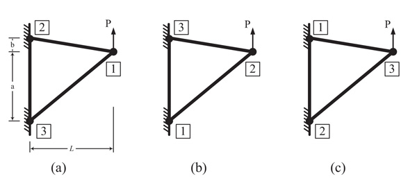
Figure 2 Three models of node numbering in spatial isotropy test.

The geometry properties of element are $L=2$, $a=0.75$ and $b=0.25$. The thickness of element is assumed to be 0.1. Moreover, the elastic modulus and Poisson’s ration are equal to $1.2\times 10^6$ and 0.0, respectively. The value of load is $P=1000$. Linear analysis is performed for these models. The obtained results, which are reported in Table 1, validate this fact.

Table 1 The results of tip displacement for spatial isotropy test

Model	Tip Displacement (v)
(a)	0.06667
(b)	0.06667
(c)	0.06667

4.2 Patch Test

Another requirement of an element is to pass the patch test. Therefore, a four-element structure is analyzed in two different states, including symmetric and asymmetric geometries. The model is shown in Figure 3. The mechanical and geometrical properties of the model are given as $E=10^5$, $v=0.3$, $D=1.0$ and $t=0.1$. The value of distributed moments is equal to $M_{xx}=M_{yy}=0.01$ N.m/m. Furthermore, the value of ${\epsilon }_0$ is assumed to be 0.0005. It should be noted that all corner nodes of structure must be fixed through z-direction in all cases ( $w_i=0i=1,2,3,4$). Three various types of loading, including, membrane, bending and mixed are considered in this model.

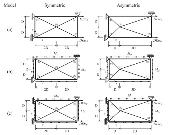
Figure 3 Patch test model, (a) membrane, (b) bending, and (c) mixed loading.

All obtained results are reported in Table 2. It is observed that the proposed element can pass this test as well.

4.3 Convergence Study

A clamped plate under the end distributed load is studied. Figure 4 shows the geometry of the model. There is an exact linear solution for the tip deflection at the free end of plate $\left(w=P{L}^3∕3EI\right)$. The module of elasticity, Poisson’s ratio and geometric properties are chosen as $E=1.2\times 10^6$, $v=0.0$, $L=10.0$, $B=1.0$ and $t=0.1$. The value of distributed load is $P=0.1$. The structure is modeled using five different mesh discretization including 2, 4, 8, 16 and 32 equivalent triangular shell elements.

Table 2 The displacement results of patch test

Case	Geometry	$u_2$	$u_3$	$v_1$	$v_2$	$w_5$
(a)	Symmetric	0.0020	0.0020	0.0003	0.0003	0.0000
	Asymmetric	0.0020	0.0020	0.0003	0.0003	0.0000
(b)	Symmetric	0.0000	0.0000	0.0000	0.0000	0.0021
	Asymmetric	0.0000	0.0000	0.0000	0.0000	0.0017
(c)	Symmetric	0.0020	0.0020	0.0003	0.0003	0.0015
	Asymmetric	0.0019	0.0019	0.0003	0.0003	0.0013

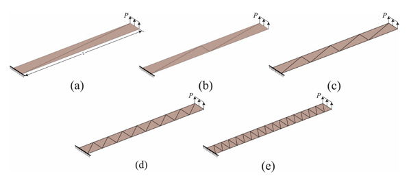
Figure 4 Mesh discretization of cantilever plate under the end distributed shear force.

All obtained responses, and the related errors are reported in Table 3. Both number of elements and DOFs are reported in this table. To show the high accuracy and convergence rate of the proposed element, the results of the tip deflection are also provided by using a 3-node triangular shell element (MITC3), in which there are no drilling degrees of freedom. In addition, the convergence rate of results is illustrated in Figure 5. It is observed that the responses achieved by proposed formulation tend to reach the exact solution by increasing the number of element. Based on these answers, it can be concluded that the element passes the consistency condition.

Table 3 The comparison results of tip deflection at the free end of clamped plate

No. of DOFs	Proposed Element	Exact Solution	Error (%)
Proposed element
24	0.250000		24.99992
36	0.312532		6.240306
60	0.328135	0.333333	1.559402
108	0.332028		0.391500
204	0.333333		0.000000
MITC3
20	0.242500		27.24993
30	0.307218		7.834221
50	0.324853	0.333333	2.543808
90	0.330035		0.989151
170	0.332999		0.100000

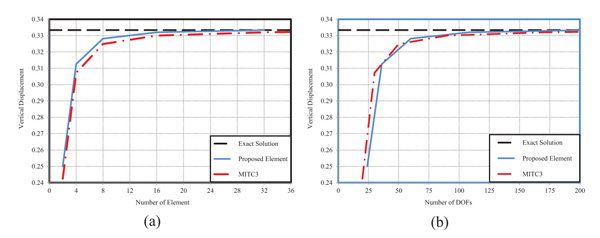
Figure 5 Convergence study of a cantilever plate under the end distributed load.

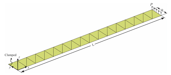
Figure 6 The initial geometry of cantilever plate under the end distributed shear force.

4.4 Cantilever Plate Under the End Distributed Shear Force

In this part, more practical structure is solved. A cantilever plate subjected to end distributed shear force, which is depicted in Figure 6, is considered in this example. This is a benchmark which has been solved previously [23]. The module of elasticity, Poisson’s ratio and geometric properties are chosen as $E=1.2\times 10^6$, $v=0.0$, $L=10.0$, $B=1.0$ and $t=0.1$.

The end distributed load is applied incrementally up to $P_{max}=4$. To obtain the results, 32 triangular elements are used for discretization. Numerical findings clearly demonstrate the high accuracy and capability of authors’ element for nonlinear analysis. The agreement between the results of present formulation and the reference solution is also excellent [23]. Figure 7 shows the load-displacement curves which are obtained for the end point of plate. Moreover, Figure 8 illustrates the deformed configuration of plate at three steps of loading including $P=0.33P_{max}$, $P=0.67P_{max}$ and $P=P_{max}$.

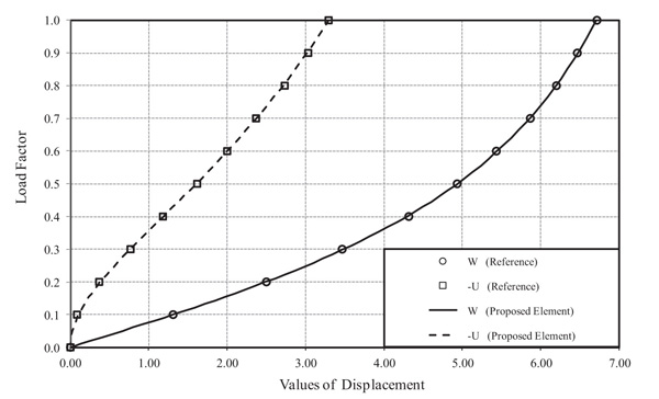
Figure 7 Load-displacement curve of cantilever plate under the end distributed shear force.

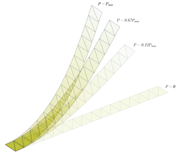
Figure 8 Deformed configurations of cantilever plate at three steps of loading.

4.5 Cantilever Plate Under the End Distributed Moment

Figure 9 shows a cantilever plate subjected to end distributed moment. To evaluate the accuracy of the proposed element, large deformation analysis of this structure, which was investigated by Jeon et al. [23], is incorporated. In this analysis, the module of elasticity and Poisson’s ratio are assumed to be $1.2\times 10^6$ and zero, respectively. The length of plate is equal to 12. Moreover, the values of width and thickness of structure are assumed to be 1.0 and 0.1, respectively.

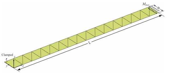
Figure 9 The initial configuration of cantilever plate under the end distributed moment.

The maximum distributed bending moment is equal to $2\pi M_0$, in which $M_0=EI∕L$. It is worth emphasizing that large rotations can be demonstrated in this problem. The analytical solution of this example corresponds to the bending classic formulations. Therefore, the deflections of cantilever plate relations are obtained as follows:

$$\begin{array}{rcll}\frac{U}{L}& =\frac{M_0}{M}sin\left(\frac{M}{M_0}\right)-1& & \\ \frac{W}{L}& =\frac{M_0}{M}\left(1-cos\left(\frac{M}{M_0}\right)\right)\end{array}$$

(30)

To show the performance of authors’ formulations, 32 triangular elements are used for the finite element discretization. Figure 10 depicted the equilibrium paths which are provided at the free end of plate. It is shown that the responses obtained by using the proposed element are in good agreement with the analytical solution determined by Equation (30). Thus, the obtained results show the capability of suggested element to analyze the large rotation and deflection problems.

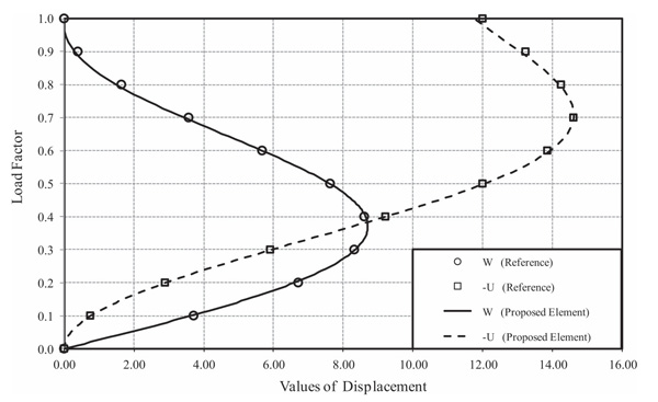
Figure 10 Equilibrium paths of cantilever plate under the end distributed moment.

4.6 Shallow Panel Under the Central Point Load

In this example, a shallow panel is modeled. The geometry and boundary conditions of structure are illustrated in Figure 11. The radius and angle $\left(\alpha \right)$ of the curve are equal to 2540 and 0.1, respectively. In addition, the thickness of structure is assumed to be 12.7. Moreover, the length of the panel is assumed to be 508. The point load which applied at the center of structure is incrementally increased up to 3500. Poisson’s ratio and elastic modulus are equal to 0.3 and 3102.75, respectively.

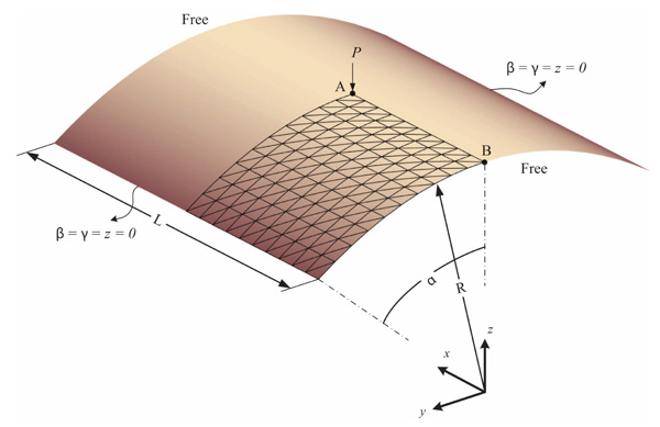
Figure 11 The geometry of shallow panel under central point load P.

Due to symmetrical geometry of structure, only a quarter of the panel is considered. The number of triangular shell element used for modeling is equal to 200. The results are depicted for points A and B in Figure 12. Comparing the obtained answers with the reference solution [44] validates the accuracy and ability of proposed element in the geometrically nonlinear analysis of shell structures. It is interesting that to obtain the correct results, which are in good agreement with reference solutions; the drilling rotations should be fixed contrary to what is thought to be. This may occur since the shell structure is shallow. On the other hand, a good improvement is observed in the obtained results in comparison with the responses achieved by using MITC3 element in which there is no drilling degree of freedom. Therefore, it is proved that the proposed formulation can improve the accuracy of the results by employing the same number of the element comparing to MITC3 element.

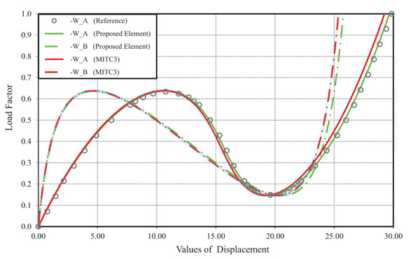
Figure 12 Load-displacement curves of shallow panel under the central point load.

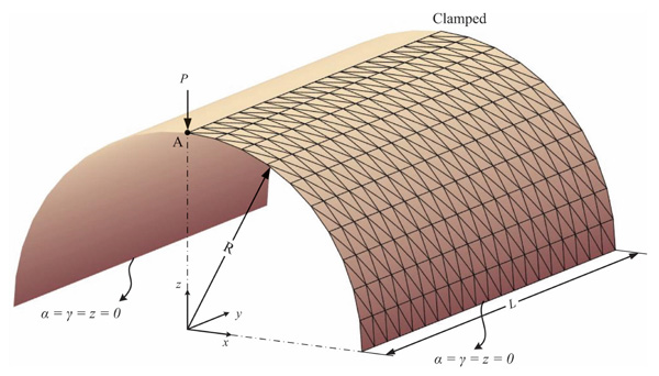
Figure 13 The initial configuration of clamped semi-cylindrical shell under the end point load.

4.7 Clamped Semi-cylindrical Shell Under the End Point Load

Another benchmark problem is a semi-cylindrical shell which is shown in Figure 13. Note that one edge of this structure is clamped while the other side is free. Moreover, the two straight sides of semi-cylindrical shell are pinned. A point load is applied at the free end of this structure. The geometry and properties of material used in this problem are given as $E=2.0685\times 10^7$, $v=0.3$, $R=1.06$, $L=0.3048$ and $t=0.03$.

The maximum load is equal to 2000. Due to symmetry, one-half of the structure is modeled. To solve the problem, 400 triangular shell elements are used for discretization. In addition, the results of horizontal and vertical displacements at the point (A) are demonstrated in Figure 14. Furthermore, these responses are compared with the available solutions [23].

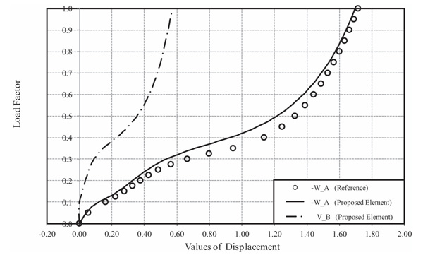
Figure 14 The equilibrium paths of clamped semi-cylindrical shell under the end point load.

4.8 Simply Supported Deep Arch

In this part, a deep semi-circular structure is modeled using 20 triangular shell elements. The initial shape of structure is shown in Figure 15. In addition, the support conditions of structure are simple.

The geometry and material properties of structure are given as $E=1378$ kPa, $v=0.0$, $t=2.7824$ cm, $B=23.1869$ cm and $R=127$ cm. The structure undertakes a distributed load $q=0.2$ N/cm at the middle. Due to symmetry, one-half of arch is modeled for analysis. The load-displacement curve of point (A) is provided in Figure 16.

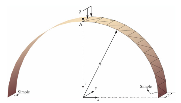
Figure 15 The geometry of simply supported deep arch.

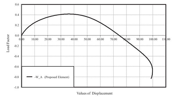
Figure 16 The equilibrium path of deep arch under the central point load P.

5 Conclusions

In this paper, a new 6-parameter triangular shell element, with drilling effect, was developed. The suggested element has three nodes, and for each of them; six degrees of freedom are considered. In fact, there are three transitional and three rotational degrees of freedom at each node. The drilling or rotational ones were defined about three director vectors, which were updated by using both updated rotation matrix and configuration of the element. To eliminate the shear and membrane locking in this element, MITC approach was employed. Besides, large displacements and rotations were incorporated in this formulation by utilizing Total Lagrangian principles. Performing comprehensive examinations demonstrated that the element can pass all the required tests. In addition, the new element was employed to solve some nonlinear popular benchmarks. Findings illustrate the capability and accuracy of this flat shell element.

Funding: This research did not receive any specific grant from funding agencies in the public, commercial, or not-for-profit sectors.

Conflict of Interest: The authors declare that they have no conflict of interest.

References

1. Ahmad, S., Irons, B., and Zienkiewicz, O. C. Analysis of thick and thin shell structures by curved finite elements. International Journal for Numerical Methods in Engineering. 1970;2:419–51.

2. Dvorkin, E. N. On nonlinear finite element analysis of shell structures: Massachusetts Institute of Technology 1984.

3. Hsiao, K. M. and Chen, Y. R. Nonlinear analysis of shell structures by degenerated isoparametric shell element. Computers and Structures. 1989;31:427–38.

4. Stanley, G. Continuum-based shell elements, Stanford, CA: Stanford University; 1985.

5. Dammak, F., Abid, S., Gakwaya, A., and Dhatt, G. A formulation of the non linear discrete Kirchhoff quadrilateral shell element with finite rotations and enhanced strains. European Journal of Computational Mechanics. 2005;14:7–31.

6. Hamadi, D., Ayoub, A., and Abdelhafid, O. A new flat shell finite element for the linear analysis of thin shell structures. European Journal of Computational Mechanics. 2015;24:232–55.

7. Mataix, V., Flores, F. G., Rossi, R., and Oñate, E. Triangular prismatic solid-shell element with generalised deformation description. European Journal of Computational Mechanics. 2018;27:1–32.

8. Bathe, K. J. and Dvorkin, E. N. A formulation of general shell elements–the use of mixed interpolation of tensorial components. International Journal for Numerical Methods in Engineering. 1986;22:697–722.

9. Dvorkin, E. N. Nonlinear Analysis of Shells Using the MITC Formulation. Archives of Computational Methods in Engineering. 1995;2:1–50.

10. Chapelle, D., Oliveira, D. L., and Bucalem, M. L. MITC elements for a classical shell model. Computers and Structures. 2003;81:523–33.

11. Rezaiee-Pajand, M., Masoodi, A. R., and Arabi, E. On the shell thickness-stretching effects using seven-parameter triangular element. European Journal of Computational Mechanics. 2018;27:163–85.

12. Rezaiee-Pajand, M. and Arabi, E. A curved triangular element for nonlinear analysis of laminated shells. Composite Structures. 2016;153:538–48.

13. Rezaiee Pajand, M., Masoodi, A., and Arabi, E. Geometrically nonlinear analysis of FG doubly-curved and hyperbolical shells via laminated by new element. Steel and Composite Structures. 2018;28:389–401.

14. Rezaiee-Pajand, M., Arabi, E., and Masoodi, A. R. Nonlinear analysis of FG-sandwich plates and shells. Aerospace Science and Technology. 2019;87:178–89.

15. Rezaiee-Pajand, M., Masoodi, A. R., and Rajabzadeh-Safaei, N. Nonlinear vibration analysis of carbon nanotube reinforced composite plane structures. Steel and Composite Structures. 2019;30:493–516.

16. Rezaiee-Pajand, M., Rajabzadeh-Safaei, N., and Masoodi, A. R. An efficient mixed interpolated curved element for geometrically nonlinear analysis. Applied Mathematical Modelling. 2019.

17. Rezaiee-Pajand, M., Rajabzadeh-Safaei, N., and Masoodi, A. R. Linear and geometrically nonlinear analysis of plane structures by using a new locking free triangular element. Engineering Structures. 2019;196:109312.

18. Lee, P. S., Noh, H. C., and Bathe, K. J. Insight into 3-node triangular shell finite elements: the effects of element isotropy and mesh patterns. Computers and Structures. 2007;85:404–418.

19. Kim, D. N. and Bathe, K. J. A triangular six-node shell element. Computers and Structures. 2009;87:1451–60.

20. Lee, Y., Yoon, K., and Lee, P. S. Improving the MITC3 shell finite element by using the Hellinger–Reissner principle. Computers and Structures. 2012;110–111:93–106.

21. Jeon, H. M., Lee, P. S., and Bathe, K. J. The MITC3 shell finite element enriched by interpolation covers. Computers and Structures. 2014;134:128–142.

22. Lee, Y., Lee, P. S., and Bathe, K. J. The MITC3 $+$ shell element and its performance. Computers and Structures. 2014;138:12–23.

23. Jeon, H. M., Lee, Y., Lee, P. S., and Bathe, K. J. The MITC3 $+$ shell element in geometric nonlinear analysis. Computers and Structures. 2015;146:91–104.

24. Rezaiee-Pajand, M., Arabi, E., and Masoodi, A. R. A triangular shell element for geometrically nonlinear analysis. Acta Mechanica. 2018;229:323–42.

25. Masoodi, A. R. and Arabi, E. Geometrically nonlinear thermomechanical analysis of shell-like structures. Journal of Thermal Stresses. 2018;41:37–53.

26. Ibrahimbegovic, A., Taylor, R. L., and Wilson, E. L. A robust quadrilateral membrane finite element with drilling degrees of freedom. International Journal for Numerical Methods in Engineering. 1990;30:445–57.

27. Iura, M. and Atluri, S. N. Formulation of a membrane finite element with drilling degrees of freedom. Computational Mechanics. 1992;9:417–28.

28. Boutagouga, D. A new enhanced assumed strain quadrilateral membrane element with drilling degree of freedom and modified shape functions. International Journal for Numerical Methods in Engineering. 2017;110:573–600.

29. Bucher, C. A family of triangular and tetrahedral elements with rotational degrees of freedom. Acta Mechanica. 2017; In Press.

30. Ibrahimbegovic, A. and Wilson, E. L. A unified formulation for triangular and quadrilateral flat shell finite elements with six nodal degrees of freedom. Communications in Applied Numerical Methods. 1991;7:1–9.

31. Gruttmann, F., Wagner, W., and Wriggers, P. A nonlinear quadrilateral shell element with drilling degrees of freedom. Archive of Applied Mechanics. 1992;62:474–86.

32. Aminpour, M. A. An assumed-stress hybrid 4-node shell element with drilling degrees of freedom. International Journal for Numerical Methods in Engineering. 1992;33:19–38.

33. Rengarajan, G., Aminpour, M. A., and Knight, N. F. Improved assumed-stress hybrid shell element with drilling degrees of freedom for linear stress, buckling and free vibration analyses. International Journal for Numerical Methods in Engineering. 1995;38:1917–43.

34. Sansour, C. and Bocko, J. On hybrid stress, hybrid strain and enhanced strain finite element formulations for a geometrically exact shell theory with drilling degrees of freedom. International Journal for Numerical Methods in Engineering. 1998;43:175–92.

35. Shin, C. M. and Lee, B. C. Development of a strain-smoothed three-node triangular flat shell element with drilling degrees of freedom. Finite Elements in Analysis and Design. 2014;86:71–80.

36. Nguyen-Van, H., Ton-That, H. L., Chau-Dinh, T., and Dao, N. D. Nonlinear static bending analysis of functionally graded plates using MISQ24 elements with drilling rotations. Singapore: Springer Singapore. 2018; pp. 461–475.

37. Kefal, A., Oterkus, E., Tessler, A., and Spangler, J. L. A quadrilateral inverse-shell element with drilling degrees of freedom for shape sensing and structural health monitoring. Engineering Science and Technology, an International Journal. 2016;19:1299–313.

38. Tang, Y. Q, Zhou, Z. H., and Chan, S. L. Geometrically nonlinear analysis of shells by quadrilateral flat shell element with drill, shear, and warping. International Journal for Numerical Methods in Engineering. 2016;108:1248–72.

39. Rezaiee-Pajand, M., Pourhekmat, D., and Arabi, E. Thermo-mechanical stability analysis of functionally graded shells. Engineering Structures. 2019;178:1–11.

40. Rezaiee-Pajand, M., Pourhekmat, D., and Arabi, E. Buckling and post-buckling of arbitrary shells under thermo-mechanical loading. Meccanica. 2019;54:205–21.

41. Lee, P. S. and Bathe, K. J. Development of MITC isotropic triangular shell finite elements. Computers and Structures. 2004;82:945–62.

42. Sussman, T. and Bathe, K.-J. 3D-shell elements for structures in large strains. Computers and Structures. 2013;122:2–12.

43. Campello, E., Pimenta, P., and Wriggers, P. A triangular finite shell element based on a fully nonlinear shell formulation. Computational Mechanics. 2003;31:505–18.

44. Arciniega, R. A. and Reddy, J. N. Tensor-based finite element formulation for geometrically nonlinear analysis of shell structures. Computer Methods in Applied Mechanics and Engineering. 2007;196:1048–73.

Biographies

Mohammad Rezaiee-Pajand received his PhD in Structural Engineering from University of Pittsburgh, Pittsburgh, PA, USA. He is currently a Professor at department of civil engineering in Ferdowsi University of Mashhad (FUM), Mashhad, Iran. His research interests are nonlinear analysis, finite element method, structural optimization and numerical techniques.

Amir R. Masoodi is a Ph.D. candidate at Ferdowsi University of Mashhad, Iran. He graduated as a B.Sc. student of Civil Engineering from Ferdowsi University of Mashhad in 2012 (Iran). He also received his M.Sc. degree of Structural Engineering (Applied Mechanics) from Ferdowsi University of Mashhad in 2014 (Iran). His interests revolve around the Nonlinear Finite Element Method (NFEM), element generation, computational mechanics, and mechanical behavior of composite materials, damage and fracture.

E. Arabi is a Ph.D. candidate at Ferdowsi University of Mashhad, Iran. He attended the Shahid Bahonar Kerman University, Iran where he received his B.Sc degree. in Civil Engineering. Elias then went on M.Sc. in Structural Engineering at the Ferdowsi University of Mashhad, Iran. His research interests are finite element analysis, mechanics of Materials, nonlinear Structural Analysis and composite Structures.

European Journal of Computational Mechanics, Vol. 28_3, 237–268.
doi: 10.13052/ejcm1958-5829.2835
© 2019 River Publishers

Abstract

Nomenclature

1 Introduction

2 Linear Kinematical Three-node Element

3 Geometrically Nonlinear Analysis

3.1 Updating Director Vectors

3.2 Incremental Displacement Field

3.3 Geometrically Nonlinear Formulation

4 Numerical Study

4.1 Isotropy Test

4.2 Patch Test

4.3 Convergence Study

4.4 Cantilever Plate Under the End Distributed Shear Force

4.5 Cantilever Plate Under the End Distributed Moment

4.6 Shallow Panel Under the Central Point Load

4.7 Clamped Semi-cylindrical Shell Under the End Point Load

4.8 Simply Supported Deep Arch

5 Conclusions

References

Biographies