Improvement of Friction Estimation Along Wellbores using Multi-scale Smoothing of Trajectories

Emilien Garcia^1,2,∗, Jacques Liandrat¹, Jacques Lessi² and Philippe Dufourcq³

¹Aix-Marseille Univ., CNRS, I2M, UMR7373, Centrale Marseille, 13451 Marseille, France
²Excellence Logging, 52-58 avenue Jean Jaurès, 92700 Colombes, France
³CentraleSupelec, Université de Paris-Saclay, 8 rue Joliot-Curie, 91190 Gif-sur-Yvette, France
E-mail: emilien.garcia@centrale-marseille.fr
^*Corresponding Author

Received 09 February 2019; Accepted 29 July 2019;
Publication 06 September 2019

Abstract

Drilling monitoring aims at anticipating and detecting drillstring failures during well construction. A key element for the monitoring activity is the estimation of friction along the wellbore trajectory. Friction models require the evaluation of the actual wellbore trajectory. This evaluation is performed applying one of many various reconstruction methods available in the industry to discrete deviation measurements. Although all these methods lead to nearly identical bit location, friction estimations are highly dependent on reconstruction methods due to huge differences in the trajectory derivatives.

To control this instability, a new reliable estimation of wellbore friction using a nonlinear trajectory smoothing process is introduced. This process uses a multi-scale approach and a specific nonlinear smoothing through subdivision schemes and their related decimation schemes. Two smoothing processes are compared: one using an interpolatory subdivision operator, and the other, a non-interpolatory subdivision operator. Validation has been performed on a synthetic plane trajectory perturbated by noise. The non-interpolatory process provides trajectory derivatives estimates much closer to those of the initial trajectory. Both processes have been applied to a real three-dimensional wellbore trajectory, improving significantly the friction estimates.

Keywords: Torque and drag, friction, drilling, trajectory, subdivision, multi-scale, smoothing

Abbreviations: T&D: Torque and Drag; PU: Pick-Up; SO: Slack-Off; FR: Free-Rotating.

1 Introduction

Well drilling is a complex activity developed for oil/gas extraction or for geothermal activities. An engineering study provides an optimal trajectory considering several objectives and constraints:

• The target objective, located according to a geological study;
• The consideration of surface constraints (environmental limitations, production platforms), which limit the possible well head locations;
• An optimal well architecture, defined from a reservoir engineering study;
• The feasibility of the drilling operations to complete the well until reaching the final target, especially ensuring limited friction inside the wellbore while tripping;
• The wellbore stability and the hydrodynamic balance throughout the drilling process, ensured through a proper mud and casing program.

The friction between the pipes and the wellbore wall is monitored through realtime discrete Hook Load and Torque surface measurements. The results of a Torque and Drag (T&D) model can then be used to match these measurements by calibrating the friction coefficients. A further discrepancy between measurements and model predictions provides a warning of potential wellbore instability or poor hole cleaning.

A T&D model is based on a friction calculation along the wellbore, so its results are very sensitive to the wellbore trajectory, in particular to the trajectory derivatives. The wellbore trajectory must be described carefully to avoid friction artefacts and consequently erroneous warnings. In practice, the trajectory is reconstructed from survey measurements collected periodically at discrete bit depths. However, results provided by T&D models are unstable due to poor approximation of trajectory derivatives.

This short summary shows that reliable trajectory reconstruction as well as stable trajectory derivatives estimates are fundamental data in the framework of wellbore monitoring.

After a short review of reconstruction methods and of friction models, Section 2 focuses on the development of a smoothing process which can provide stable derivatives estimates. Section 3 is devoted to numerical tests.

1.1 Trajectory Reconstruction

As mentioned above, a key point for drilling monitoring is the control of the trajectory, keeping in mind that the length of the well can reach 10 km. There is no direct way to accurately know the drillbit location. The data available to the directional driller are the length of the drillstring introduced inside the well and two angles measured at regular interval close to the bit. More precisely, introducing a local orthonormal coordinates system $\left(O;\overrightarrow{i},\overrightarrow{j},\overrightarrow{k}\right)$ of $R^3$ where O is the surface point at the drilling start, $\overrightarrow{i}$ (resp. $\overrightarrow{j}$) is the local horizontal unit vector pointing toward the North (resp. East), and $\overrightarrow{k}:=\overrightarrow{i}\times \overrightarrow{j}$ is the local unit vector pointing toward the Earth’s centre, the values of the following parameters ($s,\phi ,å$) are measured at each connection, i.e. before adding a pipe to the drillstring:

• The bit depth $s\in \left[0,L\right],$ where L is the forecast length of the completely drilled well. The length of each pipe of the drillstring is known within $\pm 1$ cm accuracy, but a large uncertainty remains to determine the bit depth because of pipes elongation and deformation due to their elasticity;
• The inclination angle $\phi \left(s\right)\in \left[0,\pi \right]$ and the azimuth angle $å\left(s\right)\in [0,2\pi [$ are the classical spherical coordinates angles of the bit orientation vector $\overrightarrow{t}\left(s\right)$ in the basis $\left(\overrightarrow{i},\overrightarrow{j},\overrightarrow{k}\right)$. The angle $\phi$ (resp. $å$) is known within $\pm 2^{\circ }$ (resp. $\pm 0.5^{\circ }$) accuracy.

During drilling, the available data are a sequence of triplets ${\left\{\left(s_i,{\phi }_i,{å}_i\right)\right\}}_{i=0}^n$, where $i=0$ stands for the surface condition $($usually with $\left(s_0,{\phi }_0,{å}_0\right)=\left(0,0,0\right))$ and $i=n$ stands for the last drillbit location measurement. These data can be equivalently described by the set of couples ${\left\{\left(s_i,{\overrightarrow{t}}_i\right)\right\}}_{i=0}^n$, usually with ${\stackrel{\to <!--\; \to \; -->}{t}}_0=\left(\begin{array}{c}0\\ 0\\ 1\end{array}\right)$.

The purpose of trajectory reconstruction is to build a curve $\Gamma$ starting from the origin O, given the set ${\left\{s_i,{\overrightarrow{t}}_i\right\}}_{i=0}^n$. It is constructed recursively solving the following problem: given a point $A\left(x_A,y_A,z_A\right)$ with arc length $s_A$ from O and unit tangent vector ${\overrightarrow{t}}_A$, and given the arc length $s_B$ from O and unit tangent vector ${\overrightarrow{t}}_B$ at the point B right after A, what are B’s coordinates?

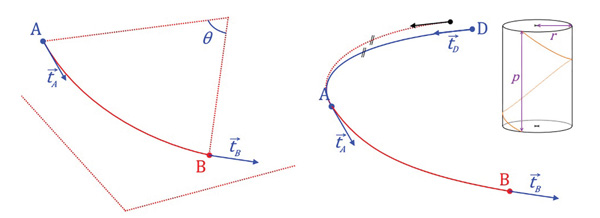
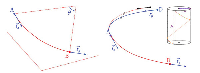
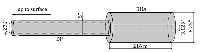
Figure 1 Reconstruction methods: left (MCM), right (MTM). Arcs AB are built using the other elements and the hypotheses of the method. For the (MTM), parameters $r$ and $p$ are respectively the radius and the pitch of the helix.

As the exact shape of the arc ${\Gamma }_{AB}$ linking A to B is not known, the problem is ill-defined and the difficulty in answering this question lies in the shape assumed for ${\Gamma }_{AB}$. Many reconstruction methods exist, each one based on different hypotheses. Following is a list of some of the existing trajectory reconstruction methods delivering trajectories at least tangentially continuous¹, that is to say $\Gamma \in {\mathcal{𝒞}}^1\left(\left[0,L\right]\right)$, where $\Gamma$ is identified as the trace of a curve $\Gamma \left(s\right)$ parametrized by its arc length $s\in \left[0,L\right]$ (see Figure 1):

• (MCM) Minimum Curvature Method (Wolff & de Wardt, 1981): ${\Gamma }_{AB}$ is the unique circular arc of the plane ($A;{\overrightarrow{t}}_A,{\overrightarrow{t}}_B$) of length $s_B-s_A$ with tangents ${\overrightarrow{t}}_A$ and ${\overrightarrow{t}}_B$ at its ends;
• (QUM) Quadratic Method (Kaplan, 2003): ${\Gamma }_{AB}$ is the unique parabolic arc of the plane ($A;{\overrightarrow{t}}_A,{\overrightarrow{t}}_B$) of length $s_B-s_A$ with tangents ${\overrightarrow{t}}_A$ and ${\overrightarrow{t}}_B$ at its ends; as tangents are interpolated between $s_A$ and $s_B$, ${\Gamma }_{AB}$ obtained by integration might have length different from $s_B-s_A$. An analytical normalization factor is then used to preserve the arc length;
• (MTM) Minimum Torsion Method (Kaplan, 2003): this method also requires $\left\{s_D,{\overrightarrow{t}}_D\right\}$ at the point D prior to A. If $\left\{{\overrightarrow{t}}_D,{\overrightarrow{t}}_A,{\overrightarrow{t}}_B\right\}$ are coplanar, ${\Gamma }_{AB}$ is the circular arc defined through (MCM); if not, ${\Gamma }_{AB}$ is assumed to be the constant-pitch helix of length $s_B-s_A$ with tangents ${\overrightarrow{t}}_A$ and ${\overrightarrow{t}}_B$ at its ends and whose extension until abscissa $s_D$ has tangent ${\overrightarrow{t}}_D$;
• (SIT) Spherical Indicatrix of Tangents 2 (Gfrerrer & Glaser, 2000): splines of order 3 interpolate tangents so that ${\Gamma }_{AB}\in {\mathcal{𝒞}}^2\left(\left[s_A,s_B\right]\right)$ is obtained by integration; however, the interpolated tangents are not necessarily of norm 1, so the integrated arc length might differ from $s_B-s_A$;
• (ASC) Advanced Spline Curve (Abughaban et al., 2016): same as (SIT) using splines of order 4, so that ${\Gamma }_{AB}\in {\mathcal{𝒞}}^3\left(\left[s_A,s_B\right]\right)$.

The application of these reconstruction methods on the same set of actual survey measurements provides discrete trajectories that are close to each other according to engineering purpose. Indeed, in all the performed simulations so far, at the same depth $s_i$, their distance measured in the $L^{\infty }$– norm remains smaller than $10$ m even when L reaches thousands of meters. Therefore, all these methods are widely acceptable and used.

Furthermore, using the interpolation based on the assumptions of each reconstruction method, the position $\Gamma \left(s\right)$ at any length $s\in \left[0,L\right]$ can be recovered, in particular on any regular segmentation ${\left\{s_i\right\}}_{i=0}^N$ of $\left[0,L\right]$. It turns out that these local interpolations are all stable and that the distance between the interpolated points remains defined within the same error of order $10$ m.

Thereafter, $\left\{\Gamma \left(s\right),0\le s\le L\right\}$ refers to an approximation of the trajectory.

1.2 Friction Model (T&D)

The friction model, usually called T&D model, is an essential mathematical and physical tool for well planning and surface monitoring (see Johancsik, Friesen & Dawson, 1983; Sheppard, 1987; Belaid, 2005; Mitchell & Samuel, 2007; Aadnoy, Fazaelizadeh & Hareland, 2010 for more details). It requires some inputs: the drill-string composition, the wellbore trajectory (defined through the vectors $\Gamma$($s$)), and many drilling parameters (mud density, drillstring angular speed and axial speed, etc.). The T&D model allows to estimate the friction factor corresponding to the Hook Load and Torque measurements while hoisting, lowering or only rotating the strings; those phases are usually called Pick-Up (PU), Slack-Off (SO) and Free Rotating (FR).

For example, the model allows to ensure that cuttings are correctly carried along the wellbore annulus (good hole cleaning), or to detect any risk of pipe getting stuck. Two friction factors are usually defined along the trajectory: $f_a$ for the axial friction and $f_r$ for the rotational friction. It is then possible to check that Hook Load and Torque values remain in correct ranges, so that the well is correctly cleaned, by comparing $f_a$ and $f_r$ to values from the literature (Samuel, 2010).

The T&D model is expressed in the local Frénet-Serret frame $\left(\overrightarrow{t},\overrightarrow{n},\overrightarrow{b}\right)$ as a function of the arc length $s\in \left[0,L\right]$ on the trajectory. As a whole, it connects the tension and moment vectors $\left(\overrightarrow{T}\left(s\right),\overrightarrow{M}\left(s\right)\right)$ at bit $\left(s=L\right)$ to their values at surface $\left(s=0\right)$ through the friction factors ($f_a,f_r$). Given two of these couples, the model provides the third one. Denoting ${\left(\cdot \right)}^{\prime }:=\frac{d\left(\cdot \right)}{ds}$, Equation (1) recalls the Frénet-Serret relations, involving the curvature $\kappa \left(s\right)$ and the torsion $\tau \left(s\right)$:

$$\frac{d}{ds}\left(\begin{array}{c}\stackrel{\to <!--\; \to \; -->}{t}\\ \stackrel{\to <!--\; \to \; -->}{n}\\ \stackrel{\to <!--\; \to \; -->}{b}\end{array}\right)=\left(\begin{array}{ccc}0& \mathrm{\kappa <!--\; \kappa \; -->}& 0\\ -<!--\; -\; -->\mathrm{\kappa <!--\; \kappa \; -->}& 0& \mathrm{\tau <!--\; \tau \; -->}\\ 0& -<!--\; -\; -->\mathrm{\tau <!--\; \tau \; -->}& 0\end{array}\right)\cdot <!--\; \cdot \; -->\left(\begin{array}{c}\stackrel{\to <!--\; \to \; -->}{t}\\ \stackrel{\to <!--\; \to \; -->}{n}\\ \stackrel{\to <!--\; \to \; -->}{b}\end{array}\right)$$

(1)

The reals $\kappa$ and $\tau$ are given by:

$$\kappa \left(s\right)=\parallel {\Gamma }^{\prime }\times {\Gamma }^{″}{\parallel }_2,\tau \left(s\right)=\frac{det\left[{\Gamma }^{\prime },{\Gamma }^{″},{\Gamma }^{‴}\right]}{{\kappa }^2},$$

(2)

and are therefore related to higher order derivatives of $\Gamma$.

In the Frénet-Serret frame, $\stackrel{\to <!--\; \to \; -->}{T}(s):=\left(\begin{array}{c}{T}_t\\ T_n\\ T_b\end{array}\right)$ and² $\stackrel{\to <!--\; \to \; -->}{M}(s)=\left(\begin{array}{c}-<!--\; -\; -->M_t\\ 0\\ E.I.k\end{array}\right)$.

The drilling fluid circulation affects the pipe tension. To consider the impact of both fluid pressures inside $\left(p_i\right)$ and outside $\left(p_o\right)$ the pipe applied on the inner $\left(S_i\right)$ and outer $\left(S_o\right)$ sections of the pipe, the “effective” pipe tension $T^{*}:=T_t+\left(p_o.S_o-p_i.S_i\right)$ is defined (cf. Mitchell, 2009 for more details).

Finally, the set of equations for the friction model used in this work is given by: (cf. Figure 2)

$$\{\begin{array}{ll}(a)& (T^{\ast <!--\; \ast \; -->}{)}^{\prime }+EI\mathrm{\kappa <!--\; \kappa \; -->}{\mathrm{\kappa <!--\; \kappa \; -->}}^{\prime }+w(\stackrel{\to <!--\; \to \; -->}{k}.\stackrel{\to <!--\; \to \; -->}{t})-<!--\; -\; -->f_a{f}_c=0,\\ (b)& (M_t{)}^{\prime }+r_o{f}_r{f}_c=0,\\ (c)& f_c=\sqrt{\frac{f_{c,n}^2+f_{c,b}^2}{1+f_r^2}},\\ (d)& f_{c,n}=w(\stackrel{\to <!--\; \to \; -->}{k}.\stackrel{\to <!--\; \to \; -->}{n})+\mathrm{\kappa <!--\; \kappa \; -->}[T^{\ast <!--\; \ast \; -->}+\mathrm{\tau <!--\; \tau \; -->}(M_t+EI\mathrm{\tau <!--\; \tau \; -->})]-<!--\; -\; -->EI{\mathrm{\kappa <!--\; \kappa \; -->}}^{″},\\ (e)& f_{c,b}=w(\stackrel{\to <!--\; \to \; -->}{k}.\stackrel{\to <!--\; \to \; -->}{b})-<!--\; -\; -->{\mathrm{\kappa <!--\; \kappa \; -->}}^{\prime }(M_t+2EI\mathrm{\tau <!--\; \tau \; -->})-<!--\; -\; -->EI\mathrm{\kappa <!--\; \kappa \; -->}{\mathrm{\tau <!--\; \tau \; -->}}^{\prime },\end{array}$$

(3)

where E is the pipes Young modulus, $I$ is the second momentum of area of the pipes, $r_0$ is the outer radius of the pipes, ${\rho }_{steel}$ is the pipe density, $\overrightarrow{w}=w\overrightarrow{k}$ is the buoyed weight per unit length of pipe, and $f_c$ is the pipe/wellbore normal contact force per unit length. These equations provide a link between the effective tension along the drillstring $T^{*}$, the torsional moment $M_t$ and the lineic pipe/wellbore contact force $f_c$ (cf. Appendix A for more details about these equations).

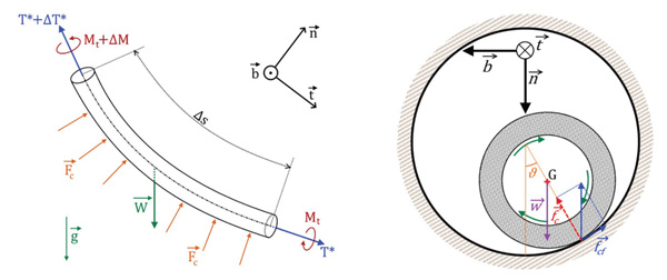
Figure 2 Left: Force balance on a pipe element. Right: Force balance for a pipe section.

This model is a Soft-String model. It is assumed that there is a continuous contact between the drillstring and the wellbore, and hence a continuous friction. Therefore, Hook Load measurements during PU and SO phases are used to calibrate $f_a$ and Torque measurements during FR phases are used to calibrate $f_r$. From Equations (3), this calibration strongly depends on the trajectory parameters $\kappa$ and $\tau$ as well as their derivatives up to ${\kappa }^{″}$ and ${\tau }^{\prime }$, so up to ${\Gamma }^{\left(4\right)}\left(s\right)$, the 4th derivative of the trajectory.

As already mentioned in Section 1.1, the estimation of the trajectory remains acceptable whatever the reconstruction method. However, even if trajectory location error is controlled regardless the trajectory reconstruction method used, the error on higher order derivatives estimation is not controlled. In particular, section by section reconstruction of the trajectory is the source of higher derivatives discontinuities at the junction points. A consequence is that the estimate of $f_a$ or $f_r$ is unstable and not accurate (see Figure 11). Moreover, there is no argument to decide if a reconstruction method provides better estimations of the trajectory derivatives than another. For instance, the regularity of the reconstruction does not imply a good estimate of the derivatives.

The proposed solution of this problem is, from an initial reconstruction $\Gamma \left(s\right)$, to construct a close trajectory with minimal oscillations, called a smooth trajectory, and to estimate the friction from this new trajectory. In particular, the smoothing process must handle higher derivatives discontinuities at junction points, as well as the noise inherent to the survey measurements.

A smoothing process that provides a trajectory of minimal oscillations must be efficient whatever the trajectory and without prior knowledge about it. This means that it is not possible to consider a linear spatial frequency filtering on the trajectory. Moreover, the objective is to control the $L^{\infty }$– error associated to the approximation of a curve and its derivatives using a polygon and its divided differences. Standard curve-fitting techniques can construct a good approximation of the trajectory, but they cannot control simultaneously its derivatives estimates.

Therefore, the non-parametric and non-linear smoothing process presented in the following section is based on a multi-scale analysis. One can prove indeed (Garcia, 2019) that if it is correctly defined, the derivatives of this smooth trajectory converges towards the derivatives of the real trajectory when the $L^{\infty }$– error between the initial reconstruction and the exact trajectory converges towards 0.

2 Multi-scale Smoothing of Trajectories

Given a discrete approximation ${\left\{\Gamma \left(s_k\right)\right\}}_{k\in Z}$ of a three-dimensional trajectory, this section presents a multi-scale smoothing acting independently on each coordinate of the trajectory. Therefore, without loss of generality, the univariate case $\left(X\left(s\right)\in R\right)$ will be considered. The sequence $X^0={\left(X^0\left(s_k\right)\right)}_{k\in Z}$, where ${\left\{s_k\right\}}_{k\in Z}\subseteq R^{+}$, is first plugged into a multi-scale framework following Harten (1996).

2.1 Multi-scale Analysis and Smoothing

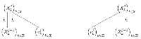
Multi-scale analysis is a mathematical tool used to represent the graph of a function $\left\{X\left(s\right),s\in R\right\}$ using different levels of approximation. Each level is characterized by the index $j\in Z$. The main ingredients of a multi-scale analysis are interscale operators linking the spaces ${\left(V^j\right)}_{j\in Z}$ standing for approximation spaces at various scales. The approximation of $X$ at level j is called $X^j$, so that $\forall k\in Z,\left(k{2}^{-j},X_k^j\right)$ approximates $\left(k{2}^{-j},X\left(k{2}^{-j}\right)\right)$. A subdivision operator $h:X^{j-1}\in V^{j-1}\mapsto h{X}^{j-1}\in V^j$ and a decimation operator $\tilde{h}:X^j\in V^j\mapsto \tilde{h}{X}^j\in V^{j-1}$, as soon as they satisfy $\tilde{h}h=Id$, define a bijection between $V^j$ and $V^{j-1}\times W^j$, where $W^j$ is the space of errors ($e^j$) (Dyn, 1992; Harten, 1996), as:

$$\left\{\begin{array}{c}{X}^{j-1}=\tilde{h}{X}^j\hfill \\ e^j=\left(Id-h\tilde{h}\right)X^j\hfill \end{array}\right.$$

(4)

Relation (4) can be inverted as $X^j=e^j+h{X}^{j-1}$. A sketch of the two-scale decomposition and reconstruction is provided on Figure 3.

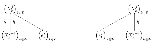
Figure 3 Two scale decomposition (left) and reconstruction (right).

Since the previous two-scale operations can be iterated, a multi-scale decomposition of a sequence $X^0$ down to level $-j_{max}<0$ can be defined as the family of sequences $\left(X^{-j_{max}},e^{-j_{max}+1},e^{-j_{max}+2},\dots ,e^{-1},e^0\right)$.

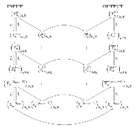
A multi-scale smoothing can be defined in 3 steps incorporating a specific error truncation. It reads, $j_{max}$ being given: (see Figure 4)

1. Multi-scale decomposition: starting from level 0, decomposition steps are iterated to reach level $-j_{max}$;
2. Error truncation: errors $e^j$ of each level are processed into new errors ${\overline{e}}^j$;
3. Multi-scale reconstruction: starting from level $-j_{max}$, reconstruction steps are iterated to reach level 0 using the errors ${\overline{e}}^j$.

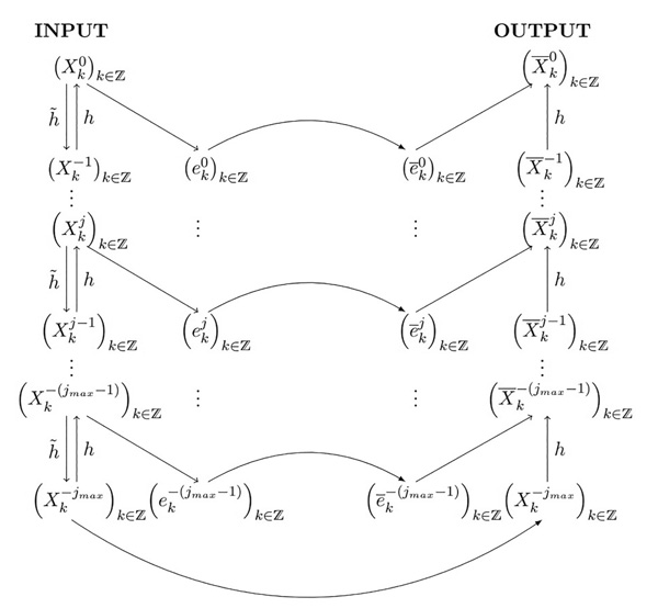
Figure 4 Structure of the multi-scale smoothing algorithm. The left part is the multi-scale decomposition (step 1), the middle part is the error truncation (step 2) and the right part is the multi-scale reconstruction (step 3).

There exists many choices for the subdivision operators and associated decimation operators (see for instance Dyn, 1992; Kui, 2018). In this paper, two subdivision operators will be used, called Lagrange interpolatory scheme (Deslauriers & Dubuc, 1989) and shifted Lagrange scheme (Dyn, Floater, & Hormann, 2005). Their definitions are given below for a 4-point stencil, as well as those of the corresponding decimations used in this paper:

4-point interpolatory Lagrange scheme

Decimation:

$${\left(\tilde{h}{X}^j\right)}_k=X_{2k}^j$$

(5)

Subdivision:

$$\left\{\begin{array}{c}{\left(h{X}^{j-1}\right)}_{2k}=X_k^{j-1}\hfill \\ & & \\ {\left(h{X}^{j-1}\right)}_{2k+1}=116\left(-X_{k-1}^{j-1}+9X_k^{j-1}+9X_{k+1}^{j-1}-X_{k+2}^{j-1}\right)\hfill \\ \hfill \end{array}\right.$$

(6)

4-point shifted Lagrange scheme

Decimation:

$$\begin{array}{rcll}{\left(\tilde{h}{X}^j\right)}_k& =& \frac{1}{2304}\left(95X_{2k-3}^j-133X_{2k-2}^j-315X_{2k-1}^j+1505X_{2k}^j\right.& \\ & & \left.+1505X_{2k+1}^j-315X_{2k+2}^j-133X_{2k+3}^j+95X_{2k+4}^j\right)& \end{array}$$

(7)

Subdivision:

$$\left\{\begin{array}{c}{\left(h{X}^{j-1}\right)}_{2k}=1128\left(-5X_{k-2}^{j-1}+35X_{k-1}^{j-1}+105X_k^{j-1}-7X_{k+1}^{j-1}\right)\hfill \\ & & \\ {\left(h{X}^{j-1}\right)}_{2k+1}=1128\left(-7X_{k-1}^{j-1}+105X_k^{j-1}+35X_{k+1}^{j-1}-5X_{k+2}^{j-1}\right)\hfill \\ \hfill \end{array}\right.$$

(8)

The specific form of (5) and of the first line of (6) explains why the first pair of schemes is called interpolatory while (7) and (8) are called non-interpolatory.

Subdivision operators can reproduce or quasi-reproduce polynomials up to a certain degree $p$ (see Kui, 2018). In particular, the subdivision scheme described by Equations (6) (resp. (8)) quasi-reproduce polynomials up to degree $p=3$ (resp. $p=4$). As both subdivision operators will be used in the multi-scale smoothing, comparison will allow to evaluate the impact of this important property on the current approach.

2.2 Error Truncation and Global Multi-scale Smoothing

Instabilities in the estimate of the derivatives are connected to the presence of “local high scale oscillations” in the reconstructions. These oscillations can be quantified considering the coefficients ${\left(a_k^j:=4^j\left(X_{k-1}^j-2X_k^j+X_{k+1}^j\right)\right)}_{k\in Z}$, which correspond to a discrete estimate at level $j$ of the second order derivative of the function $X\left(s\right)$. Indeed, a multi-scale framework is available for the coefficients ${\left(a_k^j\right)}_{k\in Z}$. For our schemes, it reads:

Interpolatory subdivision:

$$\left\{\begin{array}{c}{a}_{2k}^j=14\left(-a_{k-1}^{j-1}+6a_k^{j-1}-a_{k-1}^{j-1}\right)+4^j.\left[e_{2k-1}^j+e_{2k+1}^j\right]\hfill \\ & & \\ a_{2k+1}^j=12\left(a_k^{j-1}+a_{k+1}^{j-1}\right)-4^{j}2e_{2k+1}^j\hfill \\ \hfill \end{array}\right.$$

(9)

Non-interpolatory subdivision:

$$\left\{\begin{array}{c}{a}_{2k}^j=132\left(3a_{k-1}^{j-1}+34a_k^{j-1}-5a_{k+1}^{j-1}\right)+4^j\left[e_{2k-1}^j-2e_{2k}^j+e_{2k+1}^j\right]\hfill \\ & & \\ a_{2k+1}^j=132\left(-5a_{k-1}^{j-1}+34a_k^{j-1}+3a_{k+1}^{j-1}\right)+4^j\left[e_{2k}^j-2e_{2k+1}^j+e_{2k+2}^j\right]\hfill \\ & & \\ \hfill \end{array}\right.$$

(10)

It should be noted that the multi-scale framework described by Equations (9) is unstable and does not converge, while the one described by Equations (10) is stable and convergent. For each subdivision scheme, this result is linked to the order p for the quasi-reproduction of polynomials mentioned earlier (see Garcia, 2019).

To quantify the level of the oscillations, we introduce the notion of local scale:

Definition 2.1. For any sequence $X^0$ and any value $k_0\in Z$, the local scale $S_{k_0}$ is defined as the largest value $j$ such that there exists $\left(k_1,k_2\right)$ with: $\forall j<j^{\prime }\le 0$, such that $\forall k,k_1{2}^{-j}\le k{2}^{-j^{\prime }}\le k_2{2}^{-j},e_k^{j^{\prime }}=0$.

Clearly the sequences ${\left({\left(a_k^j\right)}_{k\in Z}\right)}_{-j_{max}\le j\le 0}$ can be seen as the result of subdivision, given by the first term of the right hand side of Equations (9) (resp. (10)), and errors, given by the second term $4^{j}A\left(e^j\right)$ of the right hand side of Equations (9) (resp. (10)). As soon as this multiresolution is stable, the norm of $a^0$ is linked (independently of $j_{max}$) to the norm of the weighted errors $4^j{e}^j$ for $-j_{max}+1\le j\le 0$. This link induces that reducing the norm of second order derivatives $a^0$ can be performed by cancelling coefficient $\left(e_k^j\right)$ with an efficiency increasing with the value of $j$.

Therefore, the error truncation of our multi-scale smoothing aims to construct a polygon ${\overline{X}}^0$ at a controlled distance of $X^0$ (i.e. $\parallel X^0-{\overline{X}}^0{\parallel }_{\infty }<ϵ)$ with a minimal local scale.

The proposed smoothing process is then sketched as follows, with the sequences $X^0$ as input and ${\overline{X}}^0$ as output:

1. Multi-scale decomposition: decomposition of the input polygon $X^0$ into the family of sequences $\left\{X^{-j_{max}},e^{-j_{max}+1},\dots ,e^0\right\}$.
2. Error truncation:
   1. Initialization: ${\overline{e}}^j:=e^j$ for all level $j\in \left\{-j_{max}+1,\dots ,0\right\}$;
   2. For $\left(j,k\right)\in \left\{-j_{max}+1,\dots ,0\right\}\times Z$ sorted such that level $j$ are in decreasing order, then non-zero $\left|{\overline{e}}_k^j\right|$ are in decreasing order (zeroes are ignored):
      • Set ${\overline{e}}_k^j=0$;
      • Multi-scale reconstruction: construct the sequence ${\overline{X}}^0$ using the sequences $\left\{X^{-j_{max}},{\overline{e}}^{-\left(j_{max}-1\right)},\dots ,{\overline{e}}^0\right\}$;
        • If $\parallel X^0-{\overline{X}}^0{\parallel }_{\infty }<ϵ$, then proceed with the next pair $\left(j^{\prime },k^{\prime }\right)$;
        • If not, set back ${\overline{e}}_k^j:=e_k^j$, then proceed with the next pair $\left(j^{\prime },k^{\prime }\right)$;
   3. If any ${\overline{e}}_k^j$ has been set to 0 during the last step (b), repeat step (b).
3. Multi-scale reconstruction: construct the output sequence ${\overline{X}}^0$ using the sequences $\left\{X^{-j_{max}},{\overline{e}}^{-\left(j_{max}-1\right)},\dots ,{\overline{e}}^0\right\}$.

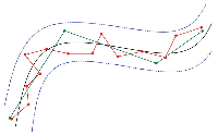
This procedure improves the estimate of the derivatives since one can prove (Garcia, 2019) that within a tube of width $ϵ>0$ around a ${\mathcal{𝒞}}^{\infty }$ curve, a polygon ${\overline{X}}^0$ of minimal local scale is such that its derivatives converge towards those of the ${\mathcal{𝒞}}^{\infty }$ curve (see Figure 5). This convergence is dependent on the existence of a stable multi-scale framework for the derivatives to study, derived from the chosen subdivision operator.

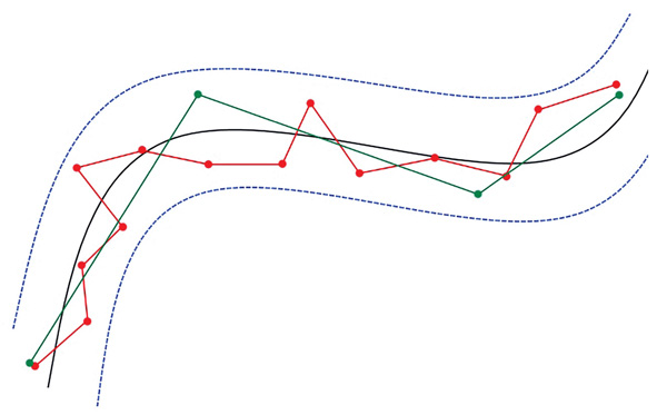
Figure 5 Polygons of different local scales. Small (resp. large) local scale is associated to the 4 points (resp. 14 points) polygon. First and second derivatives approximations using the 4 points polygon are clearly closer to the real values related to the central curve.

Remark 1. Here the whole process has been presented in the case of an infinite sequence of values $X^0={\left(X_k^0\right)}_{k\in Z}$. In practice, the process is applied on finite sequences $X^0={\left(X_k^0\right)}_{0\le k\le N}\in R^{N+1}$ for $N\in N$. In this case, the process requires adaptations at the edges of the sequences. These adaptations are presented in Appendix B.

3 Results

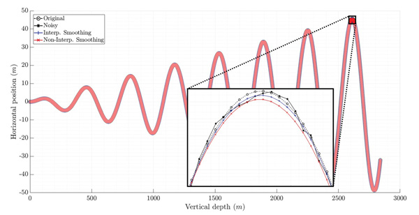
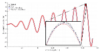
Figure 6 Comparison between the initial trajectory (dotted line with circles), the noisy trajectory (starred line) and the smoothed trajectories ($+$ line for interpolatory scheme and $\times$ line for non-interpolatory scheme). Local zoom in a high curvature region.

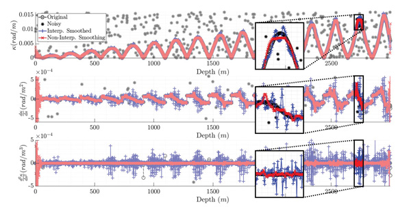
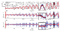
Figure 7 Comparison of the trajectory derivatives estimates along the plane trajectory, including zooms around a high curvature region (same symbols as Figure 6). From top to bottom: curvature; first derivative of the curvature; second derivative of the curvature. Noisy derivatives have such high order of magnitude that they barely appear on these graphs scales.

3.1 Application to a Noisy Known Trajectory

To validate the multi-scale smoothing process, a test plane curve is considered with constant-step segmentation on its arc length $s$. It is defined as $\left(\Gamma :=\left[X_k^0=x\left(s_k\right),Y_k^0=\frac{\pi }{180}x\left(s_k\right)sin\left(\frac{\pi }{180}x\left(s_k\right)\right)\right];s_k=k\in \left\{0,\dots ,3000\right\}\right)$. Fixing $ϵ=0.1$, a uniform noise of amplitude $0.5ϵ$ is added to $\Gamma$, and the smoothing process is applied. Then the curvature and its two first derivatives are evaluated before and after smoothing and are compared to these of the initial smooth curve. The integer $j_{max}$ is set to 6. Initial trajectory, noisy trajectory and smoothed trajectories can be seen on Figure 6. Corresponding estimates of curvature and its derivatives are plotted on Figure 7.

The comments on the results are the following:

• Curvature and its derivatives are widely overestimated when the noisy curve is used;
• Estimations of curvature and its first derivative using smoothed curves are quite similar for both subdivision schemes and very close to the original ones. The only difference between the two smoothing processes remains in some peaks, present in the interpolatory smoothing but absent in the non-interpolatory one. In both cases, these estimations are really better than the estimations without smoothing;
• Estimations of the second derivative of curvature are quite different for the two smoothing processes: the interpolatory one has a very fluctuating estimation with amplitude ten times higher than the non-interpolatory one, although this estimation is already much better than with the noisy trajectory. The non-interpolatory smoothing provides a better estimate than the interpolatory smoothing.

Globally, the smoothing is very efficient even if the interpolatory smoothing should be restricted to low order derivative estimates. The non-interpolatory smoothing seems more efficient than the interpolatory one. This could be expected in relation to the stability of the multi-scale framework up to higher order of derivatives for the non-interpolatory scheme (see comment in 2.1). Those results validate the smoothing process developed in this paper. The resulting improvement of friction estimations along a wellbore using this process is now studied.

3.2 Application to a Three-dimensional Trajectory Derived from Survey Measurements

In this section, the smoothing process is applied on reconstructed trajectories of a real wellbore. The three-dimensional trajectory $\Gamma$ considered is now described by $\mathrm{\Gamma <!--\; \Gamma \; -->}(s)=\left(\begin{array}{c}X(s)\\ Y(s)\\ Z(s)\end{array}\right)$ for $s\in <!--\; \in \; -->\{s_i{\}}_{i=0}^N$ such that $\mathrm{\Delta <!--\; \Delta \; -->}{s}_i:=s_i-<!--\; -\; -->s_{i-<!--\; -\; -->1}=1$ m for all $i\in <!--\; \in \; -->\{1,\dots <!--\; \dots \; -->,N\}$.

The smoothing process is applied to each coordinate with $ϵ=0.1$ m and $j_{max}=8$. An important difference with Section 3.1 is that the original trajectory is not known. Indeed, for this real well, the only available data are a set of measurements ${\left\{s_i,{\phi }_i,{å}_i\right\}}_{i=0}^N$ as described in Section 1.2, with no other way to estimate the trajectory than using reconstruction methods.

A reference trajectory is required to compare trajectory derivatives before and after smoothing. Since the (MCM) is the standard reconstruction method in the Oil and Gas industry and has proven its reliability on bottom hole location estimation, the (MCM) reconstructed trajectory will be considered as the reference wellbore trajectory.

Thus, (MCM) is first used for reconstruction of the reference trajectory from the set of measurements ${\left\{s_i,{\phi }_i,{å}_i\right\}}_{i=0}^N$. Then, noise is added to these survey measurements. Using the accuracy mentioned in 1.1, the noise added to each position every $10$ m of arc length is a uniform noise of amplitude $1$ cm. This noise is then cumulated for every bit depth $s_i$ throughout the wellbore. For inclination angles (resp. azimuth angles), a Gaussian noise is applied with standard deviation $\sigma =\frac{0.5}{3}$ $($resp. $\sigma =\frac{2}{3})$ centred around each measurement ${\phi }_i$ (resp. ${å}_i$).

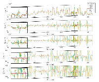
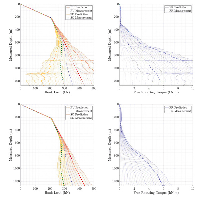
Derivatives estimates for each trajectory reconstructed from noisy survey measurements are compared. The results are given in Figure 8 for the curvature $k$ and the torsion $\tau$.

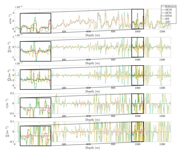
Figure 8 Comparison of the trajectory derivatives estimates along the trajectory reconstructed from noisy survey measurements. From top to bottom: curvature, first derivative of the curvature, second derivative of the curvature, torsion, and first derivative of the torsion. Each colour stands for a different reconstructed trajectory with no further smoothing.

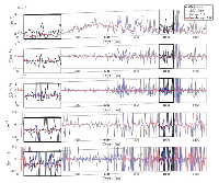
Figure 9 Comparison of the trajectory derivatives estimates using the (ASC) reconstructed trajectory. From top to bottom: curvature, first derivative of the curvature, second derivative of the curvature, torsion, and first derivative of the torsion.

The conclusions of this comparison are the following:

• Curvature estimates are close for every trajectory; however, local amplitudes in curvature derivatives can be very different for each trajectory, in particular for spline-based reconstructed trajectories (SIT and ASC) where amplitudes can be 10 times higher than for the others. Note that these trajectories are the most regular ones.
• The same dispersion for torsion and its derivative can be noted; the problem is even worse as torsion variations can be drastically different from one trajectory to another, without any way to decide if one trajectory provides better estimations than the other.

These results illustrate well the need to get a reliable method to estimate derivatives up to 4th order. To observe the efficiency of the multi-scale smoothing process, Figure 9 compares different derivatives estimates:

• From the reference trajectory reconstructed using (MCM);
• From the trajectory reconstructed from noisy measurements using (ASC);
• From interpolatory and non-interpolatory smoothings of the (ASC) trajectory reconstructed from noisy measurements.

The improvement performed by smoothing is very significant.

Again, higher derivatives estimates are better when applying the non-interpolatory scheme than when applying the interpolatory one.

3.3 Impact on Friction Estimate

Friction estimates along each wellbore trajectory are now compared. As mentioned in Equations (3), more parameters need to be defined: $E=2.1\times 10^{11}$ Pa (pipes Young modulus), ${\rho }_{steel}=7850$kg.m${}^{-3}$ (pipes density), $g=9.80665$ m.s${}^{-2}$ (gravity acceleration), $f_p={\rho }_{steel}\times g$ (pipes volumic weight), ${\rho }_{mud}=1200$ kg.m${}^{-3}$ (fluid density). Finally, the simplified and realistic drillstring used is illustrated in Figure 10.

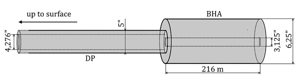
Figure 10 Illustration of the drillstring dimensions used for the simulations.

Again, the (MCM) reconstructed trajectory is chosen as the reference trajectory before adding noise to the survey measurements following Section 3.2. Using the friction model described in Equations (3) with the parameters above defined, surface pipe tension and pipe torque at different bit depths are calculated using³ $f_a^{*}=0.20$ and $f_r^{*}=0.25$. These synthetic surface parameters will be considered as reference surface measurements in the sequel. Then the T&D model is used for each trajectory (smoothed or not) reconstructed from the noisy survey measurements, varying the values of $f_a$ and $f_r$. For each trajectory, the goal is to find the pair $\left(f_a,f_r\right)$ which best matches with the surface measurements, as illustrated in Figure 11 where each line of the graphs stands for one value of the coefficient $f_a$ or $f_r$.

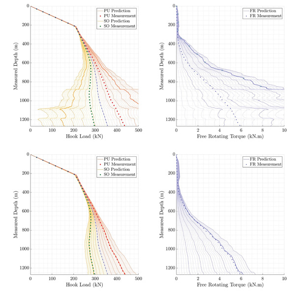
Figure 11 Torque and Tension surface measurements (dots) compared to the T&D model predictions (lines) for the (ASC) reconstructed trajectory. Each line of the graphs stands for a different friction factor from 0 to 0.30 with a 0.01 step. Predictions using the friction factors used to generate the surface data (0.20 for axial and 0.25 for rotational) are represented with bold lines on each graph. The left (resp. right) graphs are forecast surface pipe tensions (resp. surface torques) associated to different bit depths and axial movements. The upper (resp. lower) graphs are the Torque and Tension estimations from the non-smoothed (resp. smoothed) (ASC) reconstructed trajectory.

The locations of interest stand between $700$ m and $1200$ m, as there is not enough difference in surface estimations for shallower regions. The objective is far from being fulfilled before smoothing as can be seen on Figure 11, mainly for $f_r$ calibration related to (ASC) reconstruction.

As it was not possible to calibrate a single friction factor in this depth interval for all the reconstruction methods, an interval of extreme values has been determined. The corresponding results appear in Table 1.

The friction factors intervals obtained before smoothing the trajectories are very different according to the reconstruction method. For instance, friction factors are twice smaller using (SIT) than using (MCM), which is nonsense given that the bit location is the same for both trajectories.

Table 1 Calibrated friction factors intervals depending on the reconstruction method used and the subsequent smoothing applied. Real values are 0.20 for axial and 0.25 for rotational

Process	Friction	MCM-QUM	MTM	SIT	ASC
None	Axial	[0.17; 0.19]	[0.10; 0.13]	[0.04; 0.07]	[0.05; 0.08]
	Rotational	[0.21; 0.23]	[0.12; 0.17]	[0.05; 0.08]	[0.06; 0.10]
Interp.	Axial	[0.15; 0.18]	[0.14; 0.18]	[0.13; 0.17]	[0.13; 0.17]
	Rotational	[0.18; 0.23]	[0.18; 0.23]	[0.15; 0.21]	[0.12; 0.21]
Non-interp.	Axial	[0.19; 0.21]	[0.18; 0.21]	[0.18; 0.20]	[0.18; 0.20]
	Rotational	[0.23; 0.26]	[0.23; 0.26]	[0.22; 0.25]	[0.23; 0.25]

These gaps between reconstructions are much smaller after applying the interpolatory smoothing. Indeed, the coefficients intervals after smoothing now all include common values ($0.15-0.17$ for axial and $0.18-0.21$ for rotational). However, the common values do not match the values used to generate the surface data.

Using the non-interpolatory smoothing, not only the intersection of the intervals is not empty, but the values used to generate the data also belong to it. Furthermore, the interval bounds are the same for all the smoothed reconstructions. This last smoothing is therefore very efficient for friction estimations independently from the reconstruction method initially used.

For both processes, the intervals cover friction factor values higher than before applying the smoothing process, which could be expected. Indeed, the existence of a stable multi-scale framework for the divided differences is linked to the regularity of the output trajectory of the smoothing process. Since the trajectory is more regular after applying the smoothing process, smaller contact efforts are generated according to the T&D model.

4 Conclusion and Perspectives

In this paper, a new process for the evaluation of friction inside a wellbore from surface measurements has been derived. It allows a stable and satisfactory calibration of friction factors that are essential parameters for the drilling monitoring, regardless of the trajectory reconstruction initially used.

This new process is based on a multi-scale smoothing of trajectories using subdivision schemes. Tests and applications on real trajectories reveal the efficiency of the method and showed that high order subdivision schemes (here non-interpolatory Lagrange scheme) should be preferred to others.

Improvements can be proposed in different directions:

1. The choice of the tolerance $ϵ>0$ was not discussed in this publication. It could be adapted according to the local curvature along the trajectory, as developed in Garcia (2019).
2. The smoothing step currently implemented acts independently on each coordinate with the same tolerance $ϵ>0$, so it forces a point $\overline{\Gamma }\left(s_k\right)$ of the smoothed trajectory to stand in a $2ϵ$-side cube centred around $\Gamma \left(s_k\right)$. This criterion, simple to implement and already efficient, was chosen as a first approximation to test the algorithm. To include a more realistic physics of the smoothing process, the cube could be replaced by an axially oriented circular cylinder of height $h>0$ and radius $r>0$, with $r$ related to the radial clearance between the pipes and the wellbore, and $h$ linked to pipes length uncertainty.
3. Subdivision schemes with higher order $p$ for quasi-reproduction of polynomials should be used to control derivatives estimates after smoothing up to order 4 (see Garcia, 2019).

Appendix A. Friction Model

In the Serret-Frénet frame $\left(\overrightarrow{t},\overrightarrow{n},\overrightarrow{b}\right)$ associated to the wellbore trajectory, the following hypotheses are made:

• The drillstring is an elastic beam with section $S_o-S_i$, Young modulus E and second momentum of area I;
• The contact between the drillstring and the wellbore is continuous;
• Axial and rotational pipe/wellbore friction coefficients $f_a$ and $f_r$ are separately defined;
• The drilling fluid has a constant mud weight ${\rho }_{mud}$ both inside and outside the pipe;
• Viscous drag from the fluid is not considered;
• Precession angle $\vartheta$, as introduced by Mitchell & Samuel (2007) is also considered (cf. Figure 2);
• $k{r}_o<<1$ and $\tau r_o<<1$,

Efforts and momentum involved in the balances are listed below:

• Effective tension along the pipes ${\overrightarrow{T}}^{*}:=\overrightarrow{T}+\left(p_o{S}_o-p_i{S}_i\right)\overrightarrow{t}=\left(T^{*},T_n,T_b\right)$;
• Momentum of the pipes $\overrightarrow{M}=\left(-M_t,0,EI\kappa \right)$;
• Pipe buoyed lineic weight $\overrightarrow{w}=\left({\rho }_{steel}-{\rho }_{mud}\right)\left(S_o-S_i\right)g\overrightarrow{k}=\left(w_t,w_n,w_b\right)$ where ${\rho }_{steel}$ is the pipe density;
• Lineic pipe/wellbore contact normal force ${\overrightarrow{f}}_c=f_c\left(0,-cos\left(\vartheta \right),sin\left(\vartheta \right)\right)$;
• Lineic pipe/wellbore friction force ${\overrightarrow{f}}_{cf}=-f_c\left(f_a,f_{r}sin\left(\vartheta \right),f_{r}cos\left(\vartheta \right)\right)$.

Then, steady-state forces and momentum balances are given by:

$$\begin{array}{}& \{\begin{array}{l}(\stackrel{\to <!--\; \to \; -->}{T^{\ast <!--\; \ast \; -->}}{)}^{\prime }+{\stackrel{\to <!--\; \to \; -->}{f}}_c+{\stackrel{\to <!--\; \to \; -->}{f}}_{cf}+\stackrel{\to <!--\; \to \; -->}{w}=\stackrel{\to <!--\; \to \; -->}{0},\\ {\stackrel{\to <!--\; \to \; -->}{M}}^{\prime }+\stackrel{\to <!--\; \to \; -->}{t}\times <!--\; \times \; -->{\stackrel{\to <!--\; \to \; -->}{T}}^{\ast <!--\; \ast \; -->}+{\stackrel{\to <!--\; \to \; -->}{r}}_o\times <!--\; \times \; -->({\stackrel{\to <!--\; \to \; -->}{f}}_c+{\stackrel{\to <!--\; \to \; -->}{f}}_{cf})=\stackrel{\to <!--\; \to \; -->}{0}.\end{array}\end{array}$$

(A1)

According to Figure 2, ${\overrightarrow{r}}_o=r_o\left(0,cos\left(\vartheta \right),-sin\left(\vartheta \right)\right)$. Then the following system of 6 equations is obtained, by projection of Equations (A1) in the Frénet-Serret frame:

$$\{\begin{array}{l}(T^{\ast <!--\; \ast \; -->}{)}^{\prime }-<!--\; -\; -->\mathrm{\kappa <!--\; \kappa \; -->}{T}_n+w_t-<!--\; -\; -->f_a{f}_c=0,\\ T_n^{\prime }-<!--\; -\; -->\mathrm{\kappa <!--\; \kappa \; -->}{T}^{\ast <!--\; \ast \; -->}-<!--\; -\; -->\mathrm{\tau <!--\; \tau \; -->}{T}_b+w_n-<!--\; -\; -->f_c(\cos <!--\; \; -->(\mathrm{\vartheta <!--\; \vartheta \; -->})+f_r\sin <!--\; \; -->(\mathrm{\vartheta <!--\; \vartheta \; -->}))=0,\\ T_b^{\prime }+\mathrm{\tau <!--\; \tau \; -->}{T}_n+w_b+f_c(\sin <!--\; \; -->(\mathrm{\vartheta <!--\; \vartheta \; -->})-<!--\; -\; -->f_r\cos <!--\; \; -->(\mathrm{\vartheta <!--\; \vartheta \; -->}))=0,\\ -<!--\; -\; -->M_t^{\prime }-<!--\; -\; -->r_o{f}_r{f}_c=0,\\ -<!--\; -\; -->\mathrm{\kappa <!--\; \kappa \; -->}{M}_t-<!--\; -\; -->EI\mathrm{\kappa <!--\; \kappa \; -->}\mathrm{\tau <!--\; \tau \; -->}-<!--\; -\; -->T_b+r_o{f}_a{f}_c\sin <!--\; \; -->(\mathrm{\vartheta <!--\; \vartheta \; -->})=0,\\ EI{\mathrm{\kappa <!--\; \kappa \; -->}}^{\prime }+T_n+r_o{f}_a{f}_c\cos <!--\; \; -->(\mathrm{\vartheta <!--\; \vartheta \; -->})=0.\end{array}$$

(A2)

$T_n$ and $T_b$, so as $T_n^{\prime }$ and $T_b^{\prime }$, can be derived from the two last Equations of (A2):

$$\{\begin{array}{l}{T}_n=-<!--\; -\; -->EI{\mathrm{\kappa <!--\; \kappa \; -->}}^{\prime }-<!--\; -\; -->r_o{f}_a{f}_c\cos <!--\; \; -->(\mathrm{\vartheta <!--\; \vartheta \; -->}),\\ T_b=-<!--\; -\; -->\mathrm{\kappa <!--\; \kappa \; -->}{M}_t^{\prime }-<!--\; -\; -->EI\mathrm{\kappa <!--\; \kappa \; -->}\mathrm{\tau <!--\; \tau \; -->}+r_o{f}_a{f}_c\sin <!--\; \; -->(\mathrm{\vartheta <!--\; \vartheta \; -->}).\end{array}$$

(A3)

Equations (A3) are then derivated:

$$\{\begin{array}{l}{T}_n^{\prime }=-<!--\; -\; -->EI{\mathrm{\kappa <!--\; \kappa \; -->}}^{″}-<!--\; -\; -->(r_o{f}_a{f}_c\cos <!--\; \; -->(\mathrm{\vartheta <!--\; \vartheta \; -->}){)}^{\prime },\\ T_b^{\prime }=-<!--\; -\; -->{\mathrm{\kappa <!--\; \kappa \; -->}}^{\prime }(M_t+EI\mathrm{\tau <!--\; \tau \; -->})-<!--\; -\; -->\mathrm{\kappa <!--\; \kappa \; -->}{M}_t^{\prime }-<!--\; -\; -->EI\mathrm{\kappa <!--\; \kappa \; -->}{\mathrm{\tau <!--\; \tau \; -->}}^{\prime }\\ +(r_o{f}_a{f}_c\sin <!--\; \; -->(\mathrm{\vartheta <!--\; \vartheta \; -->}){)}^{\prime },\end{array}$$

(A4)

where $M_t^{\prime }$ can be replaced by its expression from the 4th Equation of (A2).

Equations (A3) Equation of (A2) and (A3) are inserted into the 4 first equations of (A2). Neglecting terms with $\kappa r_o$ and $\tau r_o$, the following system is obtained:

$$\{\begin{array}{l}{T^{\ast <!--\; \ast \; -->}}^{\prime }+EI\mathrm{\kappa <!--\; \kappa \; -->}{\mathrm{\kappa <!--\; \kappa \; -->}}^{\prime }+w_t-<!--\; -\; -->f_a{f}_c=0,\\ M_t^{\prime }+r_o{f}_r{f}_c=0,\\ w_n+\mathrm{\kappa <!--\; \kappa \; -->}(T^{\ast <!--\; \ast \; -->}+\mathrm{\tau <!--\; \tau \; -->}(M_t+EI\mathrm{\tau <!--\; \tau \; -->}))-<!--\; -\; -->EI{\mathrm{\kappa <!--\; \kappa \; -->}}^{″}-<!--\; -\; -->(r_o{f}_a{f}_c\cos <!--\; \; -->(\mathrm{\vartheta <!--\; \vartheta \; -->}){)}^{\prime }\\ =f_c(f_r\sin <!--\; \; -->(\mathrm{\vartheta <!--\; \vartheta \; -->})+\cos <!--\; \; -->(\mathrm{\vartheta <!--\; \vartheta \; -->})),\\ w_b+{\mathrm{\kappa <!--\; \kappa \; -->}}^{\prime }(M_t+2EI\mathrm{\tau <!--\; \tau \; -->})-<!--\; -\; -->EI\mathrm{\kappa <!--\; \kappa \; -->}{\mathrm{\tau <!--\; \tau \; -->}}^{\prime }+(r_o{f}_a{f}_c\sin <!--\; \; -->(\mathrm{\vartheta <!--\; \vartheta \; -->}){)}^{\prime }\\ =f_c(f_r\cos <!--\; \; -->(\mathrm{\vartheta <!--\; \vartheta \; -->})-<!--\; -\; -->\sin <!--\; \; -->(\mathrm{\vartheta <!--\; \vartheta \; -->})).\end{array}$$

(A5)

Finally, neglecting ${\left(r_o{f}_a{f}_{c}cos\left(\vartheta \right)\right)}^{\prime }$ and ${\left(r_o{f}_a{f}_{c}cos\left(\vartheta \right)\right)}^{\prime }$, 3rd and 4th equations of (A5) provide the expression of the lineic normal contact effort $f_c$. Therefore the complete system of equations is given by:

$$\{\begin{array}{l}{T^{\ast <!--\; \ast \; -->}}^{\prime }+EI\mathrm{\kappa <!--\; \kappa \; -->}{\mathrm{\kappa <!--\; \kappa \; -->}}^{\prime }+w_t-<!--\; -\; -->f_a{f}_c=0,\\ M_t^{\prime }+r_o{f}_r{f}_c=0,\\ f_c=\sqrt{\frac{[w_n+\mathrm{\kappa <!--\; \kappa \; -->}(T^{\ast <!--\; \ast \; -->}+\mathrm{\tau <!--\; \tau \; -->}(M_t+EI\mathrm{\tau <!--\; \tau \; -->}))-<!--\; -\; -->EI{\mathrm{\kappa <!--\; \kappa \; -->}}^{″}{]}^2+[w_b-<!--\; -\; -->{\mathrm{\kappa <!--\; \kappa \; -->}}^{\prime }(M_t+2EI\mathrm{\tau <!--\; \tau \; -->})-<!--\; -\; -->EI\mathrm{\kappa <!--\; \kappa \; -->}{\mathrm{\tau <!--\; \tau \; -->}}^{\prime }{]}^2}{1+f_r^2}}.\end{array}$$

(A6)

Appendix B. Adaptation of the Smoothing Algorithm to a Finite Length Input Sequence

The multi-scale analysis of a unidimensional trajectory introduced in Section 2 has entirely been developed for the case of an infinite sequence $X^0={\left(X_k^0\right)}_{k\in Z}$. In practice, the trajectory is defined through a finite sequence $X^0={\left(X_k^0\right)}_{0\le k\le N}\in R^{N+1}$. This situation requires some adaptations at the edges and some limitations linked to the number of points.

B.1. Edges Adaptations

Equations (5) to (10) involving centred stencils with 4 or 8 points are only valid for points having at least 2 or 4 neighbours at both sides. This condition is automatically fulfilled at any position for an infinite sequence of points but is no longer valid in the case of a finite sequence for points close to both ends of the sequence. Therefore, operators $h$ and $\tilde{h}$ must be redefined at edges (Kui, 2018). For sake of simplicity, only the left edge adaptation is detailed (the right edge adaptation is derived by symmetry). Equations (16) to (18) give the relations for the interpolatory and non-interpolatory schemes for the first points:

• Interpolatory initial Decimation: unchanged;
• Interpolatory initial Subdivision:

  $$\begin{array}{lll}(h{X}^{j-<!--\; -\; -->1}{)}_0& =& X_0^{j-<!--\; -\; -->1}(\text{unchanged})\\ (h{X}^{j-<!--\; -\; -->1}{)}_1& =& {\displaystyle \frac{1}{16}}(X_0^{j-<!--\; -\; -->1}-<!--\; -\; -->5X_1^{j-<!--\; -\; -->1}+15X_2^{j-<!--\; -\; -->1}+5X_3^{j-<!--\; -\; -->1})\end{array}$$

  (B1)

• Non-Interpolatory initial Decimation:

  $$\begin{array}{lll}(\stackrel{~<!--\; ~\; -->}{h}{X}^j{)}_0& =& {\displaystyle \frac{1}{16}}(5X_0^j+15X_1^j-<!--\; -\; -->5X_2^j+X_3^j)\\ (\stackrel{~<!--\; ~\; -->}{h}{X}^j{)}_0& =& {\displaystyle \frac{1}{16}}(X_0^j-<!--\; -\; -->5X_1^j+15X_2^j+5X_3^j)\end{array}$$

  (B2)

• Non-Interpolatory initial Subdivision:

  $$\begin{array}{lll}(h{X}^{j-<!--\; -\; -->1}{)}_0& =& {\displaystyle \frac{1}{128}}(195X_0^{j-<!--\; -\; -->1}-<!--\; -\; -->117X_1^{j-<!--\; -\; -->1}+65X_2^{j-<!--\; -\; -->1}-<!--\; -\; -->15X_3^{j-<!--\; -\; -->1})\\ (h{X}^{j-<!--\; -\; -->1}{)}_1& =& {\displaystyle \frac{1}{128}}(77X_0^{j-<!--\; -\; -->1}+77X_1^{j-<!--\; -\; -->1}-<!--\; -\; -->33X_2^{j-<!--\; -\; -->1}+7X_3^{j-<!--\; -\; -->1})\\ (h{X}^{j-<!--\; -\; -->1}{)}_2& =& {\displaystyle \frac{1}{128}}(15X_0^{j-<!--\; -\; -->1}+135X_1^{j-<!--\; -\; -->1}-<!--\; -\; -->27X_2^{j-<!--\; -\; -->1}+5X_3^{j-<!--\; -\; -->1})\end{array}$$

  (B3)

Similarly, $a_0^j$ must be redefined as $a_0^j=4^j\left(2X_0^j-5X_1^j+4X_2^j-X_3^j\right)$.

Given this complementary set of relations, Equations (9) and (10) expressing second derivatives ${\left(a_k^j\right)}_k$ at level $j$ as a subdivision of second derivatives ${\left(a_k^{j-1}\right)}_k$ at level $j-1$ plus errors can be generalized as follows:

Interpolatory scheme:

$$\left\{\begin{array}{c}{a}_{2k}^j=\left\{\begin{array}{c}{a}_0^{j-1}-4^j\left[5e_1^j+e_3^j\right],k=0\hfill \\ \\ 14\left(-a_{k-1}^{j-1}+6a_k^{j-1}-a_{k+1}^{j-1}\right)+4^j\left[e_{2k-1}^j+e_{2k+1}^j\right],\hfill \\ \\ k\in \left\{1,\dots ,N-1\right\}\hfill \\ \\ a_N^{j-1}-4^j\left[e_{2N-3}^j+5e_{2N-1}^j\right],k=N\hfill \end{array}\right.\hfill \\ \\ a_{2k+1}^j=12\left(a_k^{j-1}+a_{k+1}^{j-1}\right)-4^{j}2e_{2k+1}^j,k\in \left\{0,\dots ,N-1\right\}\hfill \end{array}\right.$$

(B4)

Non-interpolatory scheme:

$$\{\begin{array}{l}{a}_{2k}^j=\{\begin{array}{l}{\displaystyle \frac{1}{4}}(5a_0^{j-<!--\; -\; -->1}-<!--\; -\; -->a_1^{j-<!--\; -\; -->1})+4^j[2e_0^j-<!--\; -\; -->5e_1^j+4e_2^j-<!--\; -\; -->e_3^j],k=0\\ {\displaystyle \frac{1}{32}}(3a_{k-<!--\; -\; -->1}^{j-<!--\; -\; -->1}+34a_k^{j-<!--\; -\; -->1}-<!--\; -\; -->5a_{k+1}^{j-<!--\; -\; -->1})+4^j[e_{2k-<!--\; -\; -->1}^j-<!--\; -\; -->2e_{2k}^j+e_{2k+1}^j],\\ k\in <!--\; \in \; -->\{2,\dots <!--\; \dots \; -->,N-<!--\; -\; -->3\}\\ {\displaystyle \frac{1}{4}}(a_{k-<!--\; -\; -->1}^{j-<!--\; -\; -->1}+3a_k^{j-<!--\; -\; -->1})+4^j[e_{2k-<!--\; -\; -->1}^j-<!--\; -\; -->2e_{2k}^j+e_{2k+1}^j],\\ k=1,N-<!--\; -\; -->2,N-<!--\; -\; -->1\end{array}\\ a_{2k+1}^j=\{\begin{array}{l}{\displaystyle \frac{1}{4}}(3a_k^{j-<!--\; -\; -->1}+a_{k+1}^{j-<!--\; -\; -->1})+4^j[e_{2k}^j-<!--\; -\; -->2e_{2k+1}^j+e_{2k+2}^j],\\ k=0,1,N-<!--\; -\; -->2\\ {\displaystyle \frac{1}{32}}(-<!--\; -\; -->5a_{k-<!--\; -\; -->1}^{j-<!--\; -\; -->1}+34a_k^{j-<!--\; -\; -->1}+3a_{k+1}^{j-<!--\; -\; -->1})+4^j[e_{2k}^j-<!--\; -\; -->2e_{2k+1}^j\\ [8pt]+e_{2k+2}^j],k\in <!--\; \in \; -->\{2,\dots <!--\; \dots \; -->,N-<!--\; -\; -->3\}\\ {\displaystyle \frac{1}{4}}(-<!--\; -\; -->a_{N-<!--\; -\; -->2}^{j-<!--\; -\; -->1}+5a_{N-<!--\; -\; -->1}^{j-<!--\; -\; -->1})+4^j[-<!--\; -\; -->e_{2N-<!--\; -\; -->4}^j+4e_{2N-<!--\; -\; -->3}^j-<!--\; -\; -->5e_{2N-<!--\; -\; -->2}^j\\ +2e_{2N-<!--\; -\; -->1}^j],k=N-<!--\; -\; -->1\end{array}\end{array}$$

(B5)

B.2. Number of Values

Since the smoothing process should be applied while drilling, the number of points of the sequences is supposed to vary. In order to apply one decomposition step of the multi-scale analysis using the interpolatory (resp. non-interpolatory) schemes to a sequence of $N+1$ points, $N$ must be even (resp. odd). Iterating the argumentation, $j_{max}>0$ consecutive decomposition steps can be applied iff $\exists n\in N$ such that:

• $N+1=n\times 2^{j_{max}}+1$ using the interpolatory scheme;
• $N+1=n\times 2^{j_{max}}$ using the non-interpolatory scheme.

If $N$ does not fulfil these conditions, extra values $X_k^0$ with $k<0$ and $k>N$ can be generated and aggregated to ${\left(X_k^0\right)}_{k=0}^k\in R^{N+1}$ over the edges 0 and $N$. A linear extrapolation of degree 1 is proposed, until reaching the first number $N^{\prime }$ of values which fulfils the previous conditions. For a real three-dimensional wellbore trajectory, the new values for $k<0$ are usually given by $\left(x_k^0=0,y_k^0=0,z_k^0=k\right)$. Conversely, given $N$, the previous conditions provide an upper bound for the choice of $j_{max}$.

As noted earlier, the interpolatory smoothing is not translation invariant and does not give the same weight to every point of the trajectory. Indeed, some points are kept identical throughout the multi-scale decomposition, even if they are very noisy. Advantage can be taken from adding points at each endpoint of the trajectory, to harmonize the weights given to each point.

Supposing that $m$ values are missing from the $N+1$ values to reach the required number of values, it is possible to add $m$ values at both edges of the original trajectory ${\left(X_k^0\right)}_{k=0}^k\in R^{N+1}$, which becomes ${\left(X_k^0\right)}_{k=-m}^{N+m}\in R^{N+2m+1}$. Then, the multi-scale algorithm can be applied to each sequence of $N+m+1$ consecutive points in the set $\left\{\right.{\left(X_k^0\right)}_{k=-m+i}^{N+i};i\in \left\{0,\dots ,m\right\}\left\}\right.$. Since each sequence includes the original trajectory location $0\le k\le N$, the required smoothed trajectory can be defined as the average of all the previous smoothed sequences at these locations (after removing the 2$m$ added points for $k<0$ and $k>N$).

B.3. Adaptation for Varying Values of the Length of the Sequence

Depending on the depth of the last survey measurement, the number $N+1$ of points in the discretization of the trajectory is varying. The number $m$ of points to be generated at each endpoint of the trajectory depends on $N$, i.e. on the depth of the last survey measurement. Since $m$ is also the number of trajectories averaged at the end of the process, the quality of the smoothing process could depend on $N$.

To have a smoothing process independent from the length of the sequence, it is possible to systematically average the same number $p$ of smoothed sequences:

• $m=p:$ the current process already averages $p$ sequences to provide the required smoothed trajectory;
• $m>p:$ as more than $p$ could be averaged, a criterion must define the $p$ sequences to average; for example, the $p$ sequences that are best centred around the points ${\left(X_k^0\right)}_{k=0}^N$ can be chosen, or the $p$ sequences $\left(\right.{\left(X_k^0\right)}_{k=-m+i}^{N+i}{\left)\right.}_{i=0}^{p-1}$ in which the position of the points with $k<0$ is well known in the case of a wellbore trajectory;
• $m<p:$ this case can be treated like the case $m>p$ by extrapolating $2^{j_{max}}$ more points at each endpoint of the trajectory.

References

Aadnoy, B. S., Fazaelizadeh, M., and Hareland, G. (2010). A 3-dimensional analytical model for wellbore friction. Journal of Canadian Petroleum Technology, 49(10), 25–36.

Abughaban, M. F., Bialecki, B., Eustes, A. W., de Wardt, J. P., and Mullin, S. (2016, Mar. 1–3). Advanced trajectory computational model improves calculated borehole positioning, tortuosity and rugosity. SPE/IADC Drilling Conference, Fort Worth, Texas, SPE-178796-MS.

Belaid, A. (2005). Modélisation tridimensionnelle du comportement mécanique de la garniture de forage dans les puits à trajectoire complexe: Application à la prédiction des frottements garniture-puits (Doctoral dissertation). Retrieved from https://pastel.archives-ouvertes.fr.

Deslauriers, G., and Dubuc, S. (1989). Symmetric iterative interpolation processes. In Constr. Approx., pages 49–68, Springer.

Dyn, N. (1992). Subdivision schemes in computer aided geometric design. In W. Light, editor, Advances in Numerical Analysis II, Wavelets, Subdivision Algorithms and Radial Functions, pages 36–104. Clarendon Press, Oxford.

Dyn, N., Floater, M. S., and Hormann, K. (2005). A ${\mathcal{𝒞}}^2$ four-point subdivision scheme with fourth order accuracy and its extensions.

Garcia, E. (2019, in progress). Approche non-linéaire du monitoring de forage: Un espoir de progrès pour la commande en surface? (Unpublished doctoral dissertation). Ecole Centrale Marseille, France.

Gfrerrer, A., and Glaser, G. P. (2000). A new approach for most realistic wellpath computation. SPE, 100(3).

Harten, A. (1996). Multiresolution representation of data: A general framework. SIAM J. Numer. Anal., 33(3), 1205–1256.

Hormann, K., and Sabin, M. A. (2008). A family of subdivision schemes with cubic precision. Comput. Aided Geom. Design, 25(1), 41–52.

Johancsik, C. A., Friesen, D. B., and Dawson, R. (1983, Feb. 20–23). Torque and drag in directions wells – Prediction and measurement. SPE 11380, New Orleans, LA.

Kaplan, J. (2003). Modélisation tridimensionnelle du comportement directionnel du système de forage rotary (Doctoral dissertation). Retrieved from http://www.geosciences.mines-paristech.fr/fr.

Kui, Z. (2018). On the construction of multiresolution analysis compatible with general subdivisions (Doctoral dissertation). Retrieved from https://pastel.archives-ouvertes.fr.

Mitchell, R. F., and Samuel, R. (2007, Feb. 21–23). How good is the torque drag model? Paper SPE 105068 presented at the IADC/SPE Drilling Conference, Miami, Florida, USA.

Mitchell, R. F. (2009, Mar. 17–19). Fluid momentum balance defines the effective force. Paper SPE/IADC 119954 presented at the 2009 SPE/IADC Drilling Conference and Exhibition, Amsterdam, the Netherlands.

Samuel, R. (2010). Friction factor: What are they for torque, drag, vibration, bottom hole assembly and transient surge/swab analyses. J. Pet. Sci. Eng., 73.

Sheppard, M. C. (1987, Oct. 5–8). Designing well path to reduce torque and drag. SPE 15463, New Orleans, LA.

Si, X., Baccou, J., and Liandrat, J. (2016). On four-point penalized Lagrange subdivision schemes. Applied Mathematics and Computation, 281, 278–299.

Wolff, C. J. M., and de Wardt, J. P. (1981). Borehole position uncertainty – Analysis of measuring methods and derivation of systematic error model. Journal of Petroleum Technology, 33(12), 2339–2350.

Biographies

Emilien Garcia graduated from both Ecole Centrale Marseille (Marseille, France) and Universidad de Chile (Santiago, Chile). He holds a PhD in Mathematics since June 2019.

Jacques Liandrat graduated from Ecole Polytechnique (Palaiseau, France) in 1981. He got his Ph.D in 1986 from Sup-Aero/Université Paul Sabatier (Toulouse, France). Since 1993 he is full professor in mathematics at Ecole Centrale Marseille (Marseille, France).

Jacques Lessi has more than 40 years of experience in Research and Development related to oil & gas upstream industry, both in public research for 22 years and in service company for the last 18 years. His main competencies are related to formation evaluation both for fluid content and rock mineralogy characterization, drilling efficiency, vibration detection and mitigation, wellbore stability and hydraulic balance. He has authored along his career several international publications and about 25 patents (20 US patent presently issued). He graduated from the Ecole des Mines de Paris and holds a PhD from the University of Strasbourg.

Philippe Dufourcq PhD and Engineering Graduate from Ecole Centrale de Lyon, he began his career with ten years in companies, notably in Thales. He joined higher education as Chairman of Research at the Ecole Supérieure d’Ingénieurs in Marseille, before being appointed Director of Development at Ecole Centrale de Marseille. For several years he led its strategic orientation committee and his academic senate, before joining Morocco to launch the Ecole Centrale Casablanca of which he was the first Director of Programs. Since 1 January 2019, he has held the position of Deputy Chief Executive Officer of CentraleSupelec. His areas of research and teaching concern the physics of complex systems.

¹Since the trajectory is generated by a tangentially continuous drillstring, the trajectory should at least have the same regularity.

²The tangential component of $\overrightarrow{M}$ is defined with the minus sign to count positively the surface momentum.

³In practice, calibrated $f_a^{*}$ and $f_r^{*}$ are not equal to each other.

European Journal of Computational Mechanics, Vol. 28_3, 207–236.
doi: 10.13052/ejcm1958-5829.2834
© 2019 River Publishers

Abstract

1 Introduction

1.1 Trajectory Reconstruction

1.2 Friction Model (T&D)

2 Multi-scale Smoothing of Trajectories

2.1 Multi-scale Analysis and Smoothing

2.2 Error Truncation and Global Multi-scale Smoothing

3 Results

3.1 Application to a Noisy Known Trajectory

3.2 Application to a Three-dimensional Trajectory Derived from Survey Measurements

3.3 Impact on Friction Estimate

4 Conclusion and Perspectives

Appendix A. Friction Model

Appendix B. Adaptation of the Smoothing Algorithm to a Finite Length Input Sequence

B.1. Edges Adaptations

B.2. Number of Values

B.3. Adaptation for Varying Values of the Length of the Sequence

References

Biographies