A Finite Element Formulation for Kirchhoff Plates in Strain-gradient Elasticity

Alireza Beheshti

Department of Mechanical Engineering, University of Guilan, Rasht, Iran E-mail: beheshti.arza@gmail.com

Received 09 February 2019; Accepted 31 July 2019;
Publication 21 August 2019

Abstract

The current contribution is centered on bending of rectangular plates using the finite element method in the strain-gradient elasticity. To this aim, following introducing stresses and strains for a plate based on the Kirchhoff hypothesis, the principle of the virtual work is adopted to derive the weak form. Building upon Hermite polynomials and by deeming convergence requirements, four rectangular elements for the static analysis of strain-gradient plates are presented. To explore the performance of the proposed elements, particularly in small scales, some problems are solved and the results are compared with analytical solutions.

Keywords: Strain-gradient Elasticity, Finite Element Method, Kirchhoff plate.

1 Introduction

Albeit the classical continuum mechanics is valid for most analyses in large scales, it fails for problems in small scales. There are some evidences for shortcomings of the classical mechanics (Stolken and Evans, 1998; Hutchinson, 2000; Lam, Yang, Chong, Wang and Tong, 2003; Haque and Saif, 2003). Fleck, Muller, Ashby and Hutchinson (1994) conducted some experiments on the plastic torsion of wires in small scales and showed that the stiffness of the material is higher than the prediction of the classical mechanics. The strain-gradient theory elaborated by Mindlin (1964) and Mindlin and Eshel (1968) is able to predict the response of an object in the small scale accurately (Aifantis, 2003). It is worthy of note that Mindlin (1964) firstly developed the theory of elasticity with microstructure by the inclusion of a micro-volume in a particle defined in the macro-medium. Finally, by making some assumptions, three simpler models were derived from the original theory of elasticity with microstructure. Aifantis (1992) proposed the simple, robust model in which the only unconventional material constant is the so-called material length-scale parameter. Due to its simplicity and robustness, the model has been widely used in the analyses associated with the strain-gradient elasticity (Ru and Aifantis, 1993; Aifantis, 2009; Aravas, 2011; Beheshti, 2017a).

The static analysis of plates in the gradient elasticity has been addressed by some researchers. Papargyri-Beskou and Beskos (2008) extracted the partial differential equations as well as the boundary conditions for a flexural plate allowing for the Kirchhoff model and provided analytical solutions to the simply supported rectangular plate. Later, Lazopoulos (2009) developed a formulation for the bending of strain-gradient Kirchhoff plates and derived the differential equation and boundary conditions. Further, building upon the strain-gradient elasticity model presented by Lam et al. (2003), Wang, Zhou, Zhao and Chen (2011) studied the size-dependent behavior of simply-supported Kirchhoff plates analytically.

It should be pointed out that analytical techniques often work on simple geometries, boundary conditions, and loadings specially for strain-gradient elasticity in which the gradient of the strain tensor plays an important role. Consequently, a reliable numerical method is an asset for solving complex problems. In this paragraph, the most important works in the numerical analysis of gradient elasticity are introduced briefly. Shu, King and Fleck (1999) and subsequently Amanatidou and Aravas (2002) developed mixed finite element formulations based on C⁰ interpolation functions for the analysis of two-dimensional strain-gradient solids. In Papanicolopulos, Zervos and Vardoulakis (2009), a C¹ -continuous finite element for the three dimensional analysis of solids was developed. Fischer, Mergheim and Steinmann (2010) made use of three different C¹ -continuous finite elements to analyze the large deformation of strain-gradient solids and compared their results with those based C¹ Natural Element Method. Askes, Morata and Aifantis (2008) split the fourth-order equations of gradient elasticity into two sets of second-order equations and devised C⁰ strain-gradient elements. Furthermore, use was made of the Hermite polynomials to elaborate high-order elements for the deformation analysis of solids, bars, beams, and plates by Beheshti (2016, 2017b, 2018a, b). Additionally, the Isogeometric Analysis has also been used in the analyses associated with the gradient elasticity. In this regard, Niiranen, Kiendl, Niemi and Reali (2017) addressed the sixth-order boundary value problem connected with the gradient Kirchhoff plate in bending using the Galerkin-type isogeometric analysis. Interested readers on numerical schemes in strain-gradient elasticity are recommended to study Tsinopoulos, Polyzos and Beskos (2012) and Singh, Nair, Rajagopal, Pal and Pandey (2018).

The objective of the current contribution is presenting four novel rectangular elements for the bending analysis of rectangular plates with an emphasis on the convergence requirements. In Section 2, building upon the Kirchhoff plate model, the strain field and then the stress field accounting for the constitutive equations in the strain-gradient elasticity are derived. Section 3 in which the weak form for the bending of the strain-gradient plate is given is followed by Section 4 that is centered on the finite element formulation of the problem and introducing the rectangular elements. Afterwards, some numerical examples are solved by using the developed elements in Section 5. Finally, a conclusion is presented in Section 6.

2 Kirchhoff Plate Model

In this section, building upon the Kirchhoff plate model along with constitutive equations in the strain-gradient elasticity, the strains, strain-gradients, stresses and double stresses for the bending of a plate are presented. Also, for the notational convenience, it is supposed that, in the present contribution, Greek subscripts take the values of 1 and 2 and Latin subscripts take the values of 1, 2 and 3.

2.1 Components of Strain Tensors

In the Kirchhoff plate model, which is widely used for this plates, cross sections normal to the midsurface in the underformed state remains straight and perpendicular to the deformed midsurface after deformation. Additionally, it is assumed that the thickness of the plate does not alter during the deformation. These simplifications yield following strain field (Ugural, 1981):

$${\mathrm{\epsilon <!--\; \epsilon \; -->}}_{\mathrm{\alpha <!--\; \alpha \; -->}\mathrm{\beta <!--\; \beta \; -->}}=-<!--\; -\; -->x_3{w}_{,\mathrm{\alpha <!--\; \alpha \; -->}\mathrm{\beta <!--\; \beta \; -->}},$$

(1)

where w is the deflection of the midsurafce. Also, it must be noted that the axis x₃ is in the thickness direction and the x₁ x₂ -plane coincides with the middle plane.

To proceed with the derivation of strains, it should be noted that the gradient of the infinitesimal strain tensor, ξ_ijk = ɛ_jk,i, features prominently in the Form II of the strain-gradient theories developed by Mindlin (1964) and Mindlin and Eshel (1968). The non-vanishing components of the strain-gradient tensor are

$${\mathrm{\xi <!--\; \xi \; -->}}_{\mathrm{\gamma <!--\; \gamma \; -->}\mathrm{\alpha <!--\; \alpha \; -->}\mathrm{\beta <!--\; \beta \; -->}}=-<!--\; -\; -->x_3{w}_{,\mathrm{\gamma <!--\; \gamma \; -->}\mathrm{\alpha <!--\; \alpha \; -->}\mathrm{\beta <!--\; \beta \; -->}},{\mathrm{\xi <!--\; \xi \; -->}}_{3\mathrm{\alpha <!--\; \alpha \; -->}\mathrm{\beta <!--\; \beta \; -->}}=-<!--\; -\; -->w_{,\mathrm{\alpha <!--\; \alpha \; -->}\mathrm{\beta <!--\; \beta \; -->}}.$$

(2)

Now, all non-zero components of strain and strain-gradient tensors are accomplished and by inserting them in constitutive equations stress and double stress tensors are achieved.

2.2 Components of Stress Tensors

Building upon the aforementioned strain field, it is very straight-forward to extract the stress field allowing for the strain-stress relations in the linear elasticity. For the analysis of a thin plate, the following stress field can be presented (Ugural, 1981):

$$\begin{array}{rl}{\mathrm{\sigma <!--\; \sigma \; -->}}_{11}& =\frac{E}{(1-<!--\; -\; -->{\mathrm{\nu <!--\; \nu \; -->}}^2)}[{\mathrm{\epsilon <!--\; \epsilon \; -->}}_{11}+\mathrm{\nu <!--\; \nu \; -->}{\mathrm{\epsilon <!--\; \epsilon \; -->}}_{22}],{\mathrm{\sigma <!--\; \sigma \; -->}}_{22}=\frac{E}{(1-<!--\; -\; -->{\mathrm{\nu <!--\; \nu \; -->}}^2)}[\mathrm{\nu <!--\; \nu \; -->}{\mathrm{\epsilon <!--\; \epsilon \; -->}}_{11}+{\mathrm{\epsilon <!--\; \epsilon \; -->}}_{22}],\\ {\mathrm{\sigma <!--\; \sigma \; -->}}_{12}& =\frac{E}{(1+\mathrm{\nu <!--\; \nu \; -->})}{\mathrm{\epsilon <!--\; \epsilon \; -->}}_{12}.\end{array}$$

(3)

As for the double stress tensor, the nonzero components are (Aravas, 2011)

$$\begin{array}{rl}{\mathrm{\mu <!--\; \mu \; -->}}_{i11}& =\frac{E{l}^2}{(1-<!--\; -\; -->{\mathrm{\nu <!--\; \nu \; -->}}^2)}[{\mathrm{\xi <!--\; \xi \; -->}}_{i11}+\mathrm{\nu <!--\; \nu \; -->}{\mathrm{\xi <!--\; \xi \; -->}}_{i22}],{\mathrm{\mu <!--\; \mu \; -->}}_{i22}=\frac{E{l}^2}{(1-<!--\; -\; -->{\mathrm{\nu <!--\; \nu \; -->}}^2)}[\mathrm{\nu <!--\; \nu \; -->}{\mathrm{\xi <!--\; \xi \; -->}}_{i11}+{\mathrm{\xi <!--\; \xi \; -->}}_{i22}],\\ {\mathrm{\mu <!--\; \mu \; -->}}_{i12}& =\frac{E}{(1+\mathrm{\nu <!--\; \nu \; -->})}{\mathrm{\xi <!--\; \xi \; -->}}_{i12}.\end{array}$$

(4)

where l is the so-called material length scale parameter in the strain-gradient elasticity.

It is worthwhile to note that the stress-strain relations above are on basis of simple, robust strain gradient theory proposed by Aifantis (1992). In the model, the components of the double-stress tensor are

$${\mathrm{\mu <!--\; \mu \; -->}}_{ijk}=l^2(\mathrm{\lambda <!--\; \lambda \; -->}{\mathrm{\delta <!--\; \delta \; -->}}_{jk}{\mathrm{\xi <!--\; \xi \; -->}}_{ipp}+2G{\mathrm{\xi <!--\; \xi \; -->}}_{ijk}),$$

(5)

where λ stands for the Lame’s constant and G is the shear modulus.

3 Variational Formulation

To derive the weak form associated with the small deformation of a plate in bending, the principle of virtual work (PVW) is adopted in current contribution. For the static state, PVW says that the variation of the strain energy is equal to the variation of the work done by external loadings, δU = δW . The variation of the strain energy for the strain-gradient plate reads

$$\mathrm{\delta <!--\; \delta \; -->}U={\int <!--\; \int \; -->}_v\{{\mathrm{\sigma <!--\; \sigma \; -->}}_{\mathrm{\alpha <!--\; \alpha \; -->}\mathrm{\beta <!--\; \beta \; -->}}\mathrm{\delta <!--\; \delta \; -->}{\mathrm{\epsilon <!--\; \epsilon \; -->}}_{\mathrm{\alpha <!--\; \alpha \; -->}\mathrm{\beta <!--\; \beta \; -->}}+{\mathrm{\mu <!--\; \mu \; -->}}_{i\mathrm{\alpha <!--\; \alpha \; -->}\mathrm{\beta <!--\; \beta \; -->}}\mathrm{\delta <!--\; \delta \; -->}{\mathrm{\xi <!--\; \xi \; -->}}_{i\mathrm{\alpha <!--\; \alpha \; -->}\mathrm{\beta <!--\; \beta \; -->}}\}\underset{dAd{x}_3}{\underset{⏟<!--\; ⏟\; -->}{dV}}.$$

(6)

By considering the stress and strain fields, it is plausible to integrate the relation above over the thickness direction. Before proceeding with the procedure, let us introduce the following resultants:

$$M_{\mathrm{\alpha <!--\; \alpha \; -->}\mathrm{\beta <!--\; \beta \; -->}}={\int <!--\; \int \; -->}_t{\mathrm{\sigma <!--\; \sigma \; -->}}_{\mathrm{\alpha <!--\; \alpha \; -->}\mathrm{\beta <!--\; \beta \; -->}}{x}_{3}d{x}_3,S_{\mathrm{\gamma <!--\; \gamma \; -->}\mathrm{\alpha <!--\; \alpha \; -->}\mathrm{\beta <!--\; \beta \; -->}}={\int <!--\; \int \; -->}_t{\mathrm{\mu <!--\; \mu \; -->}}_{\mathrm{\gamma <!--\; \gamma \; -->}\mathrm{\alpha <!--\; \alpha \; -->}\mathrm{\beta <!--\; \beta \; -->}}{x}_{3}d{x}_3,P_{3\mathrm{\alpha <!--\; \alpha \; -->}\mathrm{\beta <!--\; \beta \; -->}}={\int <!--\; \int \; -->}_t{\mathrm{\mu <!--\; \mu \; -->}}_{3\mathrm{\alpha <!--\; \alpha \; -->}\mathrm{\beta <!--\; \beta \; -->}}d{x}_3,$$

(7)

where t stands for the thickness of the plate.

It is beneficial to arrange relations above in the matrix form for the FE formulation. Hence, the total resultant vector is made of the aforementioned resultants. It is

$$\mathbf{\text{Q}}=\{{\stackrel{~<!--\; ~\; -->}{\mathbf{\text{M}}}}^T,{\stackrel{~<!--\; ~\; -->}{\mathbf{\text{S}}}}^T,{\stackrel{~<!--\; ~\; -->}{\mathbf{\text{P}}}}^T{\}}^T,$$

(8)

with

$$\begin{array}{rcl}\stackrel{~<!--\; ~\; -->}{\mathbf{\text{M}}}& =& \{M_{11},M_{22},M_{12}{\}}^T,\stackrel{~<!--\; ~\; -->}{\mathbf{\text{S}}}=\{S_{111},S_{122},S_{211},S_{222},S_{112},S_{212}{\}}^T,\\ \stackrel{~<!--\; ~\; -->}{\mathbf{\text{P}}}& =& \{P_{311},P_{322},P_{312}{\}}^T.\end{array}$$

(9)

Additionally, the resultant vectors can be expressed by

$$\stackrel{~<!--\; ~\; -->}{\mathbf{\text{M}}}=-<!--\; -\; -->{\mathbf{\text{D}}}_1{\mathrm{\kappa <!--\; \kappa \; -->}}_1,\stackrel{~<!--\; ~\; -->}{\mathbf{\text{S}}}=-<!--\; -\; -->{\mathbf{\text{D}}}_2{\mathrm{\kappa <!--\; \kappa \; -->}}_2,\stackrel{~<!--\; ~\; -->}{\mathbf{\text{P}}}=-<!--\; -\; -->{\mathbf{\text{D}}}_3{\mathrm{\kappa <!--\; \kappa \; -->}}_1,$$

(10)

where the material matrices are

$$\begin{array}{lll}{\mathbf{\text{D}}}_1& =& \frac{t^2}{12l^2}{\mathbf{\text{D}}}_3=D\left[\begin{array}{ccc}1& \mathrm{\nu <!--\; \nu \; -->}& 0\\ \mathrm{\nu <!--\; \nu \; -->}& 1& 0\\ 0& 0& (1-<!--\; -\; -->\mathrm{\nu <!--\; \nu \; -->})/2\end{array}\right],\\ {\mathbf{\text{D}}}_2& =& D{l}^2\left[\begin{array}{cccccc}1& \mathrm{\nu <!--\; \nu \; -->}& 0& 0& 0& 0\\ \mathrm{\nu <!--\; \nu \; -->}& 1& 0& 0& 0& 0\\ 0& 0& 1& \mathrm{\nu <!--\; \nu \; -->}& 0& 0\\ 0& 0& \mathrm{\nu <!--\; \nu \; -->}& 1& 0& 0\\ 0& 0& 0& 0& (1-<!--\; -\; -->{\mathrm{\nu <!--\; \nu \; -->}}^2)/2& 0\\ 0& 0& 0& 0& 0& (1-<!--\; -\; -->{\mathrm{\nu <!--\; \nu \; -->}}^2)/2\end{array}\right],\end{array}$$

(11)

D = Et³/12(1 – ν²) is the flexural rigidity of the plate and the strain vectors are

	$\begin{array}{lll}{\mathrm{\kappa <!--\; \kappa \; -->}}_1& =& \{w_{,11},w_{,22},2w_{,12}{\}}^T,\end{array}$	(12)
	$\begin{array}{rcl}{\mathrm{\kappa <!--\; \kappa \; -->}}_2& =& \{w_{,111},w_{,122},w_{112},w_{,222},2w_{,112},2w_{,122}{\}}^T.\end{array}$	(13)

In addition, by substituting Equation (10) in Equation (8), the alternative form of the total resultant vector is accomplished as follows:

$$\mathbf{\text{Q}}=-<!--\; -\; -->\mathbf{\text{D}}\mathrm{\kappa <!--\; \kappa \; -->}$$

(14)

with

$$\mathbf{\text{D}}=\left[\begin{array}{ccc}{\mathbf{\text{D}}}_1& \mathbf{\text{0}}& \mathbf{\text{0}}\\ \mathbf{\text{0}}& {\mathbf{\text{D}}}_2& \mathbf{\text{0}}\\ \mathbf{\text{0}}& \mathbf{\text{0}}& {\mathbf{\text{D}}}_3\end{array}\right]\mathrm{a}\mathrm{n}\mathrm{d}\mathrm{\kappa <!--\; \kappa \; -->}=\{{\mathrm{\kappa <!--\; \kappa \; -->}}_1^T,{\mathrm{\kappa <!--\; \kappa \; -->}}_2^T,{\mathrm{\kappa <!--\; \kappa \; -->}}_1^T{\}}^T.$$

(15)

Finally, the variational strain energy can be rewritten in the following form:

$$\mathrm{\delta <!--\; \delta \; -->}U={\int <!--\; \int \; -->}_A\mathrm{\delta <!--\; \delta \; -->}{\mathrm{\kappa <!--\; \kappa \; -->}}^T\mathbf{\text{D}}\mathrm{\kappa <!--\; \kappa \; -->}dA.$$

(16)

As for the variational external work, it reads

$$\mathrm{\delta <!--\; \delta \; -->}\mathit{W}={\int <!--\; \int \; -->}_{A}p\mathrm{\delta <!--\; \delta \; -->}wdA$$

(17)

where p is the distributed, transverse load exerted to the middle surface of the plate.

The matrix form of the variational strain energy and the variational external work ease construction of the stiffness matrix and the load vector in the finite element method presented in the next section.

4 Finite Element Formulation

In this section, all procedures associated with the development of the elements for the static analysis of a plate in the gradient elasticity are presented. Following introduction of the approximated deflections of the plate based on the finite element method, the associated shape functions for the four rectangular plate elements are presented. Subsequently, by exploiting the relations derived in the previous section, the stiffness matrix and the load vector are submitted. Two issues should be dealt with herein. The novelty of present work is attributed to the four rectangular plate elements for static analysis of Kirchhoff plates in the strain-gradient elasticity. It is crucial to mention that a majority of finite element analyses conducted in the area of gradient elasticity are centered on two- and three-dimensional solids and beams. Also, the data presented in the numerical section can be used by future studies for comparison purposes and for checking the performance of the proposed elements, results from the FE plates are compared with analytical solutions in detail.

4.1 Displacement Approximation

Without dealing with details, we directly focus on the approximated displacement for the four-node rectangular elements designed in the current contribution. Recall from textbooks in finite element method that three requirements should be satisfied to construct a reliable, accurate element (Hughes, 1987). Briefly, those are continuation of a variable in the element and more importantly in the element boundaries and completeness of shape functions. In the present work, we base the shape functions on the Hermite polynomials and try to explore the convergence of the rectangular elements allowing for the requirements. Four rectangular plate elements with three, four, six and nine degrees of freedom per node are presented herein and those are abbreviated to P3, P4, P6 and P9, respectively. It is worthy of note that the four nodal points are in the corners of the rectangle. Furthermore, it must be pointed out that we do not define a parent element in the current FE formulation and the elements are defined with respect to the local coordinate system located in the bottom left corner of the rectangular element. The approximated field can be introduced as follows:

$$w_e^{\ast <!--\; \ast \; -->}={\sum <!--\; \sum \; -->}_{i=1}^2{\sum <!--\; \sum \; -->}_{j=1}^2{\mathbf{\text{H}}}_{ij}^{\ast <!--\; \ast \; -->T}{\mathbf{\text{w}}}_{ij}^{\ast <!--\; \ast \; -->},$$

(18)

where the asterisk must be replaced with P3, P4, P6 and P9.

Furthermore, the shape function vectors are

	$\begin{array}{lll}{\mathbf{\text{H}}}_{ij}^{P3}& =& \{H_{0i}^{11}{H}_{0j}^{12},H_{1i}^{11}{H}_{0j}^{12},H_{0i}^{11}{H}_{1j}^{12}{\}}^T,\end{array}$	(19)
	$\begin{array}{lll}{\mathbf{\text{H}}}_{ij}^{P4}& =& \{H_{0i}^{11}{H}_{0j}^{12},H_{1i}^{11}{H}_{0j}^{12},H_{0i}^{11}{H}_{1j}^{12},H_{1i}^{11}{H}_{1j}^{12}{\}}^T,\end{array}$	(20)
	$$\begin{array}{rcl}{\mathbf{\text{H}}}_{ij}^{P6}& =& \{H_{0i}^{11}{H}_{0j}^{12},H_{1i}^{11}{H}_{0j}^{12},H_{0i}^{11}{H}_{1j}^{12},H_{1i}^{11}{H}_{1j}^{12},H_{2i}^{21}{H}_{0j}^{22},H_{0i}^{21}{H}_{2j}^{22}{\}}^T,\\ & & \end{array}$$	(21)
	$\begin{array}{rcl}{\mathbf{\text{H}}}_{ij}^{P9}& =& \{H_{0i}^{11}{H}_{0j}^{12},H_{1i}^{11}{H}_{0j}^{12},H_{0i}^{11}{H}_{1j}^{12},H_{1i}^{11}{H}_{1j}^{12},H_{2i}^{21}{H}_{0j}^{22},H_{0i}^{21}{H}_{2j}^{22},\\ & & H_{2i}^{21}{H}_{1j}^{22},H_{1i}^{21}{H}_{2j}^{22},H_{2i}^{21}{H}_{2j}^{22}{\}}^T,\end{array}$	(22)

and the nodal generalized-displacement vectors have the following forms for every element:

$\begin{array}{rcl}{\mathbf{\text{w}}}_{ij}^{P3}& =& \{w_{ij},w_{,1_{ij}},w_{,2_{ij}}{\}}^T,\end{array}$

(23)

$\begin{array}{rcl}{\mathbf{\text{w}}}_{ij}^{P4}& =& \{w_{{}_{ij}},w_{,1_{ij}},w_{,2_{ij}},w_{,{12}_{ij}}{\}}^T,\end{array}$	(24)
$\begin{array}{rcl}{\mathbf{\text{w}}}_{ij}^{P6}& =& \{w_{ij},w_{,1_{ij}},w_{,2_{ij}},w_{,{12}_{ij}},w_{,{11}_{ij}},w_{,{22}_{ij}}{\}}^T,\end{array}$	(25)
$$\begin{array}{rcl}{\mathbf{\text{w}}}_{ij}^{P9}& =& \{w_{ij},w_{,1_{ij}},w_{,2_{ij}},w_{,{12}_{ij}},w_{,{11}_{ij}},w_{,{22}_{ij}},w_{,{112}_{ij}},w_{,{122}_{ij}},w_{,{1122}_{ij}}{\}}^T.\end{array}$$	(26)

Also, the subscripts i and j appearing in the above relations determine the node position in the rectangular elements, see Figure 1. For instance, the pair (2,2) indicates that the corresponding node is located in the top right corner of the rectangular element.

As for the above-mentioned shape functions, the Hermite polynomials are taken into account. Suppose that two points are located on the axis x_γ , γ is an integer (say 1 or 2), one is at the origin and the other is at the distance of aγ from the origin in the positive direction. The following one-dimensional functions accounting for imposed conditions on the third-order and fifth-order polynomials and their derivatives can be presented (Bogner, Fox and Schmit, 1966).

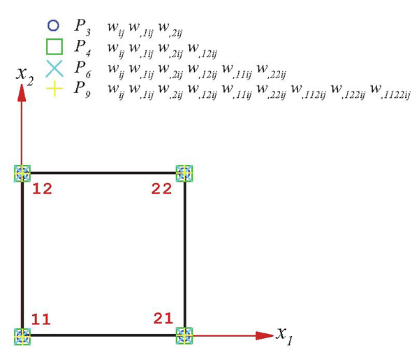
Figure 1 Rectangular plate elements.

$$\begin{array}{rcl}& & H_{01}^{1\mathrm{\gamma <!--\; \gamma \; -->}}=(2x_{\mathrm{\gamma <!--\; \gamma \; -->}}^3-<!--\; -\; -->3a_{\mathrm{\gamma <!--\; \gamma \; -->}}{x}_{\mathrm{\gamma <!--\; \gamma \; -->}}^2+a_{\mathrm{\gamma <!--\; \gamma \; -->}}^3)/a_{\mathrm{\gamma <!--\; \gamma \; -->}}^3,H_{02}^{1\mathrm{\gamma <!--\; \gamma \; -->}}=-<!--\; -\; -->(2x_{\mathrm{\gamma <!--\; \gamma \; -->}}^3-<!--\; -\; -->3a_{\mathrm{\gamma <!--\; \gamma \; -->}}{x}_{\mathrm{\gamma <!--\; \gamma \; -->}}^2)/a_{\mathrm{\gamma <!--\; \gamma \; -->}}^3,\\ & & H_{11}^{1\mathrm{\gamma <!--\; \gamma \; -->}}=(x_{\mathrm{\gamma <!--\; \gamma \; -->}}^3-<!--\; -\; -->2a_{\mathrm{\gamma <!--\; \gamma \; -->}}{x}_{\mathrm{\gamma <!--\; \gamma \; -->}}^2+a_{\mathrm{\gamma <!--\; \gamma \; -->}}^2{x}_{\mathrm{\gamma <!--\; \gamma \; -->}})/a_{\mathrm{\gamma <!--\; \gamma \; -->}}^2,H_{12}^{1\mathrm{\gamma <!--\; \gamma \; -->}}=(x_{\mathrm{\gamma <!--\; \gamma \; -->}}^3-<!--\; -\; -->a_{\mathrm{\gamma <!--\; \gamma \; -->}}{x}_{\mathrm{\gamma <!--\; \gamma \; -->}}^2)/a_{\mathrm{\gamma <!--\; \gamma \; -->}}^2,\end{array}$$

(27)

and

$$\begin{array}{rcl}{H}_{01}^{2\mathrm{\gamma <!--\; \gamma \; -->}}& =& (a_{\mathrm{\gamma <!--\; \gamma \; -->}}^5-<!--\; -\; -->10a_{\mathrm{\gamma <!--\; \gamma \; -->}}^2{x}_{\mathrm{\gamma <!--\; \gamma \; -->}}^3+15a_{\mathrm{\gamma <!--\; \gamma \; -->}}{x}_{\mathrm{\gamma <!--\; \gamma \; -->}}^4-<!--\; -\; -->6x_{\mathrm{\gamma <!--\; \gamma \; -->}}^5)/a_{\mathrm{\gamma <!--\; \gamma \; -->}}^5,\\ H_{02}^{2\mathrm{\gamma <!--\; \gamma \; -->}}& =& (10a_{\mathrm{\gamma <!--\; \gamma \; -->}}^2{x}_{\mathrm{\gamma <!--\; \gamma \; -->}}^3-<!--\; -\; -->15a_{\mathrm{\gamma <!--\; \gamma \; -->}}{x}_{\mathrm{\gamma <!--\; \gamma \; -->}}^4+6x_{\mathrm{\gamma <!--\; \gamma \; -->}}^5)/a_{\mathrm{\gamma <!--\; \gamma \; -->}}^5,\\ H_{11}^{2\mathrm{\gamma <!--\; \gamma \; -->}}& =& (a_{\mathrm{\gamma <!--\; \gamma \; -->}}^4{x}_{\mathrm{\gamma <!--\; \gamma \; -->}}-<!--\; -\; -->6a_{\mathrm{\gamma <!--\; \gamma \; -->}}^2{x}_{\mathrm{\gamma <!--\; \gamma \; -->}}^3+8a_{\mathrm{\gamma <!--\; \gamma \; -->}}{x}_{\mathrm{\gamma <!--\; \gamma \; -->}}^4-<!--\; -\; -->3x_{\mathrm{\gamma <!--\; \gamma \; -->}}^5)/a_{\mathrm{\gamma <!--\; \gamma \; -->}}^4,\\ H_{12}^{2\mathrm{\gamma <!--\; \gamma \; -->}}& =& (-<!--\; -\; -->4a_{\mathrm{\gamma <!--\; \gamma \; -->}}^2{x}_{\mathrm{\gamma <!--\; \gamma \; -->}}^3+7a_{\mathrm{\gamma <!--\; \gamma \; -->}}{x}_{\mathrm{\gamma <!--\; \gamma \; -->}}^4-<!--\; -\; -->3x_{\mathrm{\gamma <!--\; \gamma \; -->}}^5)/a_{\mathrm{\gamma <!--\; \gamma \; -->}}^4,\\ H_{21}^{2\mathrm{\gamma <!--\; \gamma \; -->}}& =& (a_{\mathrm{\gamma <!--\; \gamma \; -->}}^3{x}_{\mathrm{\gamma <!--\; \gamma \; -->}}^2-<!--\; -\; -->3a_{\mathrm{\gamma <!--\; \gamma \; -->}}^2{x}_{\mathrm{\gamma <!--\; \gamma \; -->}}^3+3a_{\mathrm{\gamma <!--\; \gamma \; -->}}{x}_{\mathrm{\gamma <!--\; \gamma \; -->}}^4-<!--\; -\; -->x_{\mathrm{\gamma <!--\; \gamma \; -->}}^5)/2a_{\mathrm{\gamma <!--\; \gamma \; -->}}^3,\\ H_{22}^{2\mathrm{\gamma <!--\; \gamma \; -->}}& =& (a_{\mathrm{\gamma <!--\; \gamma \; -->}}^2{x}_{\mathrm{\gamma <!--\; \gamma \; -->}}^3-<!--\; -\; -->2a_{\mathrm{\gamma <!--\; \gamma \; -->}}{x}_{\mathrm{\gamma <!--\; \gamma \; -->}}^4+x_{\mathrm{\gamma <!--\; \gamma \; -->}}^5)/2a_{\mathrm{\gamma <!--\; \gamma \; -->}}^3.\end{array}$$

(28)

Recall that the local coordinate system is at the left, bottom corner of the rectangular element so that x₁ and x₂ are parallel to the horizontal and vertical axes, respectively. Thus, a₁ and a₂ are the element length along x₁ and x₂ axes, respectively. For finding details about the derivation of the Hermite polynomials above, refer to the work of Bogner, Fox and Schmit (1966). Clearly, by multiplication of the one-dimensional Hermite polynomials, the appropriate shape functions for the analysis of the plate are derived.

4.2 Stiffness Matrix and Load Vector

As noted before, in the FE formulation herein no parent space is defined and all calculations are defined with respect to the local coordinate system in each element. In addition to the local coordinate system, it is assumed that there is a global coordinate system that is aligned with the local ones.

The first step for extracting the stiffness matrix is inserting the approximated deflection field, i.e. Equation (18), into the strain vectors, i.e. Equations (12) and (13), then the result in the total strain vector κ. It yields that W_e is the element generalized-displacement vector. Note that for convenience, the superscript associated with the element type has been eliminated.

$${\mathrm{\kappa <!--\; \kappa \; -->}}_e={\mathbf{\text{BW}}}_e,$$

(29)

with

$${\mathbf{\text{W}}}_e=\{{\mathbf{\text{w}}}_{11},{\mathbf{\text{w}}}_{12},{\mathbf{\text{w}}}_{22},{\mathbf{\text{w}}}_{21}{\}}^T,$$

(30)

By inserting Equation (29) into Equation (16), the variational strain energy for every element can be obtained

$$\begin{array}{rcl}\mathrm{\delta <!--\; \delta \; -->}{U}_e& =& {\int <!--\; \int \; -->}_{A_e}\mathrm{\delta <!--\; \delta \; -->}{\mathrm{\kappa <!--\; \kappa \; -->}}_e^T\mathbf{\text{D}}{\mathrm{\kappa <!--\; \kappa \; -->}}_{e}d{x}_{1}d{x}_2=\mathrm{\delta <!--\; \delta \; -->}{\mathbf{\text{W}}}_e^T{\mathbf{\text{K}}}_e{\mathbf{\text{W}}}_e\mathrm{w}\mathrm{i}\mathrm{t}\mathrm{h}\\ {\mathbf{\text{K}}}_e& =& {\int <!--\; \int \; -->}_{A_e}{\mathbf{\text{B}}}^T\mathbf{\text{DB}}d{x}_{1}d{x}_2,\end{array}$$

(31)

where K_e is the stiffness matrix for a typical element. It worthy of note that a definite analytical integration is implemented to calculate the stiffness matrix rather than a numerical integration. By applying the same procedure, the force vector for an element can be derived. It reads

$$\begin{array}{rcl}\mathrm{\delta <!--\; \delta \; -->}{\mathit{W}}_e& =& \mathrm{\delta <!--\; \delta \; -->}{\mathbf{W}}_e^T{F}_e\mathrm{w}\mathrm{i}\mathrm{t}\mathrm{h}{\mathbf{F}}_e={\int <!--\; \int \; -->}_{A_e}p{\mathbf{H}}_{e}d{x}_{1}d{x}_2\mathrm{a}\mathrm{n}\mathrm{d}\\ {\mathbf{H}}_e& =& \{{\mathbf{H}}_{11}^T,{\mathbf{H}}_{21}^T,{\mathbf{H}}_{22}^T,{\mathbf{H}}_{12}^T{\}}^T\end{array}$$

(32)

Finally, by bearing in mind the principle of the virtual work, the final matrix equation is KW = F where K, F and W are the assembled stiffness matrix, the assembled load vector, and the assembled generalized-displacement vector, respectively.

4.3 Convergence Requirements

In this section, the requirements associated with the convergence of elements are studied in detail. Those involve the continuity of the field in the element, continuity of the field along the element interfaces, and completeness of the variable. The first requirement is not challenging and it is easily satisfied for all elements developed herein. However, the last two conditions are not very simple to fulfill. Thus, a topic has been devoted to those.

4.3.1 P3 element

For the element with three degrees of freedom per node, by expanding the approximated field for the deflection of the plate it is concluded that, in the element interface, the deflection is a function of nodal DoF in the same interface, accordingly continuous between two adjacent elements. Also it must be mentioned that the first normal derivatives of the deflection is continuous along the common side, but the second normal derivatives do not satisfy the compatibility of the element. Another crucial topic is that the proposed polynomial for the deflection does not meet the completeness condition, in the sense presented by Bogner, Fox and Schmit (1966), i.e.$w(x_1,x_2)=\underset{r=0}{\overset{\stackrel{¯<!--\; ¯\; -->}{r}}{\sum <!--\; \sum \; -->}}\underset{s=0}{\overset{\stackrel{¯<!--\; ¯\; -->}{s}}{\sum <!--\; \sum \; -->}}{\mathrm{\alpha <!--\; \alpha \; -->}}_{rs}{x}_1^r{x}_2^s$ where $\stackrel{¯<!--\; ¯\; -->}{r}$ and $\stackrel{¯<!--\; ¯\; -->}{s}$ are the maximum power of x and y in the approximated field.

4.3.2 P4 element

Let us focus on the element with four degrees of freedom per node. For this case, the polynomial used to approximate the deflection is complete. But the second normal derivative of the deflection is not continuous along the common sides. Accordingly, the element does not satisfy the compatibility condition. It must be pointed out that the major difference of the element with the P3 element is the completeness.

4.3.3 P6 element

It should be noted that the major idea of increasing the number of degrees of freedom is satisfying the compatibility of elements given the highest order of derivatives appearing in the weak form. The investigation into the element P6 exhibits that it is continuous but incomplete. Thus, it fails to meet all convergence requirements.

4.3.4 P9 element

Let us concentrate on the element P9. The element is not only compatible but also complete. That is to say, deflection and its first and second derivatives in every interface are defined with respect to the degrees of freedom in the common nodes only, hence continuous along the common side. On the account of the fact that the variational index is 3 in Equation (6) it is necessary to fulfill the C²-continuity of the deflection in order to pass the compatibility requirement. It is expected that the element is the most accurate one in the current analysis. The critical information about the performance of the elements is exposed in the numerical analyses.

5 Numerical Results

To explore the performance and validity of the proposed elements for the small deformation analysis of the strain-gradient plates, some problems are solved and the results are compared with the analytical strain-gradient and classical solutions. In such a way, not only the convergence of the elements is studied but also the size-dependent behavior of plates in small scales are taken into account. For reporting the result of plate deformation conveniently, a non-dimensional displacement $\stackrel{¯<!--\; ¯\; -->}{w}$ is defined. It is$\stackrel{¯<!--\; ¯\; -->}{w}$ =$\stackrel{¯<!--\; ¯\; -->}{w}=1000wD/P{a}^2$ and$\stackrel{¯<!--\; ¯\; -->}{w}=1000wD/p{a}^4$ for a square plate under the point force, P, and the pressure, p, respectively. Further, in all analyses conducted in this section, it is supposed that plates are squares with the length a and the ratio of length to thickness is a/t = 100 satisfying the thin plate condition. In all examples, the material parameters are E = 200 GPa, ν =0.3 and l =0.1 mm (Bagni, Askes and Susmel, 2016). In addition, we focus on two types of boundary conditions involving simply-supported and clamped ones. The former and the latter for an edge along the x₂ axis are defined as follows:

	$\begin{array}{rcl}w& =& w_{,2}=w_{,22}=0,\end{array}$	(33)
	$\begin{array}{rcl}w& =& w_{,2}=w_{,22}=w_{,1}=w_{,12}=w_{,122}=0.\end{array}$	(34)

By replacement of the subscript 1 with 2 and vice versa above the relation is modified for an edge along x₁ axis.

The nondimensional deflection of plates in different sizes is provided for various elements in some tables. In addition, it is worth noting that the result of different meshes has also been included in the tables.

5.1 Simply Supported Square Plates

The first example is about the deformation of simply supported plates. Since the analytical solution for this type of plates is available to us, see the Appendix, the problem is of great importance. In other words, the accuracy and performance of all elements can be checked and the finite element results can be compared with the analytical solutions. Two various loadings involving the pressure and the central point force are considered and central non-dimensional displacements are tabulated in Tables 1 and 2. Further, the deformed shape of the plate under the loadings has been shown in Figure 2. In these tables, in addition to the finite element solution for various meshes and elements, the analytical strain-gradient and classical responses are also incorporated.

The absolute error value of the element P3 is around 5 per cent for both cases involving distributed and terminal loadings, hence it fails to predict the response of the plates. As for the element P4, for both loads, the results are stiffer than the analytical data and relative error is about 0.3%. For the distributed and concentrated loadings, the element P6 has the error of approximately –0.01% and –0.02%, respectively. Finally, the element P9 that meets all convergence requirements bears almost no error, say 0.001 percent.

Table 1 The nondimensional deflection of the plates at the center for simply supported plates under pressure

t/l	Element Type	Number of Elements						$\stackrel{¯<!--\; ¯\; -->}{w}$ASG	$\stackrel{¯<!--\; ¯\; -->}{w}$C† (Ugural, 1981)
		4×4	8×8	12×12	16×16	20×20	24×24
1	P3	0.2926	0.2962	0.2966	0.2963	0.2958	0.2951	0.3124	4.06
	P4	0.3097	0.3102	0.3108	0.3112	0.3114	0.3115
	P6	0.3118	0.3123	0.3124	0.3124	0.3124	0.3124
	P9	0.3125	0.3125	0.3125	0.3125	0.3125	0.3125
2	P3	0.9510	0.9628	0.9642	0.9637	0.9625	0.9607	1.0155	4.06
	P4	1.0067	1.0083	1.0103	1.0114	1.0120	1.0125
	P6	1.0134	1.0149	1.0152	1.0153	1.0154	1.0154
	P9	1.0155	1.0155	1.0155	1.0155	1.0155	1.0155
8	P3	3.2041	3.2454	3.2525	3.2543	3.2544	3.2537	3.4208	4.06
	P4	3.3913	3.3971	3.4040	3.4078	3.4102	3.4119
	P6	3.4140	3.4188	3.4199	3.4203	3.4205	3.4206
	P9	3.4209	3.4209	3.4209	3.4209	3.4209	3.4209
128	P3	3.8024	3.8519	3.8611	3.8643	3.8658	3.8666	4.0594	4.06
	P4	4.0244	4.0313	4.0395	4.0442	4.0471	4.0491
	P6	4.0512	4.0570	4.0583	4.0587	4.0590	4.0591
	P9	4.0594	4.0594	4.0594	4.0594	4.0594	4.0594

^† The superscript C stands for the classical solution.

The note the draws much attention is that the element P9 is completely convergent even for small number of elements. Accordingly, the disadvantage of the element which is high number of DoF is balanced by lower number of elements. Further, as can be verified, it is the most accurate element, see Figures 3 and 4 in which the relative error of the finite element method building upon the central displacement is depicted versus total number of nodes.

Let us focus on the size-dependent behavior of the strain-gradient plates. As is clear in Tables 1 and 2, by gradually increasing the ratio t/l, the strain- gradient results tend towards the classical solutions, whereas for the small value of t/l the strain-gradient response is stiffer than the classical one. That is, in the case in which size of structure is sufficiently large, the classical and strain-gradient results are identical.

Table 2 The central nondimensional deflection for simply supported plates under concentrated force at the center

t/l	Element Type	Number of Elements						$\stackrel{¯<!--\; ¯\; -->}{w}$ASG	$\stackrel{¯<!--\; ¯\; -->}{w}$C (Ugural, 1981)
		4×4	8×8	12×12	16×16	20×20	24×24
1	P3	0.8294	0.8458	0.8484	0.8484	0.8474	0.8458	0.8919	11.59
	P4	0.8745	0.8847	0.8875	0.8887	0.8893	0.8897
	P6	0.8869	0.8905	0.8913	0.8916	0.8917	0.8918
	P9	0.8911	0.8918	0.8919	0.8919	0.8919	0.8919
2	P3	2.6957	2.7495	2.7586	2.7594	2.7571	2.7530	2.8989	11.59
	P4	2.8421	2.8755	2.8846	2.8885	2.8906	2.8919
	P6	2.8826	2.8945	2.8969	2.8978	2.8982	2.8985
	P9	2.8962	2.8985	2.8988	2.8989	2.8990	2.8990
8	P3	9.0831	9.2688	9.3059	9.3180	9.3220	9.3221	9.7679	11.59
	P4	9.5755	9.6888	9.7199	9.7337	9.7414	9.7462
	P6	9.7117	9.7522	9.7607	9.7639	9.7654	9.7662
	P9	9.7578	9.7658	9.7672	9.7677	9.7679	9.7680
128	P3	10.7792	11.0009	11.0471	11.0644	11.0727	11.0774	11.5921	11.59
	P4	11.3631	11.4979	11.5350	11.5516	11.5609	11.5668
	P6	11.5248	11.5731	11.5833	11.5870	11.5888	11.5899
	P9	11.5796	11.5892	11.5909	11.5915	11.5918	11.5920

Figure 2 Deformed shape of a simply supported plate under (a) pressure (b) point load.

5.2 Clamped Square Plates

This example is concerned with the bending of square plates that are clamped in all four sides. Similar to the preceding example, two types of the loading including the uniform distributed load and the terminal force at the center are taken into account, see Figure 5. Let us begin with the element P3 that is the simplest element. As can be predicted and is visible in the Tables 3 and 4, the element is not able to estimate the deflection of the plate accurately and the corresponding error is about –3 per cent. For the distributed loading, interestingly, the result of the elements P4 and P9 are completely similar. However, the element P9 is less sensitive to the mesh, so that the results do not alter by increasing the elements from 16 to 576. Also, notice that the elements are distributed evenly along the x₁ and x₂ axes. Additionally, it should be emphasized that for the point force the P4 provides us with the stiffer results, say the error is 0.05 per cent. By comparing the results of the element P6 with the convergent element P9 in the Tables 3 and 4, it is deduced that the relative error of the P6 is -0.04% approximately.

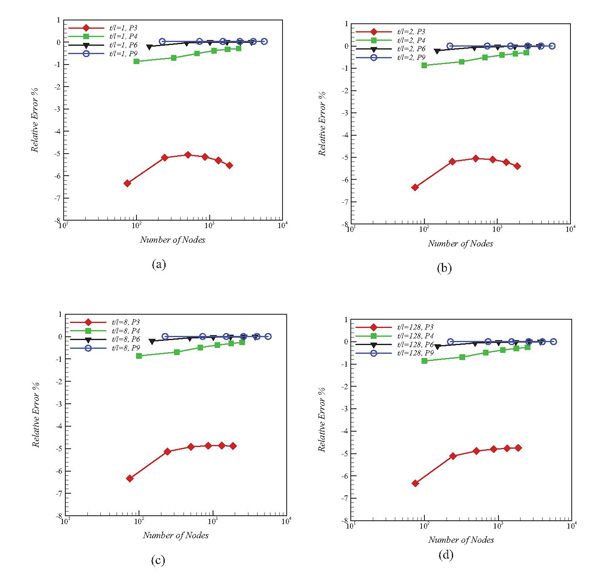
Figure 3 Mesh convergence study on a plate under pressure for (a) t/l =1(b) t/l = 2 (c) t/l =8(d) t/l = 128.

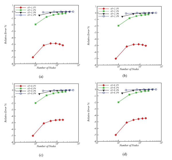
Figure 4 Mesh convergence study on a plate under central point force for (a) t/l =1 (b) t/l =2(c) t/l =8(d) t/l = 128.

Figure 5 Deformed shape of a clamped plate under (a) pressure (b) point load.

Table 3 The nondimensional deflection of the plate at the center for clamped plates under pressure

t/l	Element Type	Number of Elements						$\stackrel{¯<!--\; ¯\; -->}{w}$C (Ugural, 1981)
		4×4	8×8	12×12	16×16	20×20	24×24
1	P3	0.0931	0.0943	0.0946	0.0947	0.0947	0.0946	1.26
	P4	0.0972	0.0973	0.0973	0.0973	0.0973	0.0973
	P6	0.0966	0.0971	0.0972	0.0972	0.0973	0.0973
	P9	0.0973	0.0973	0.0973	0.0973	0.0973	0.0973
2	P3	0.3027	0.3064	0.3077	0.3080	0.3080	0.3079	1.26
	P4	0.3161	0.3162	0.3162	0.3162	0.3162	0.3162
	P6	0.3141	0.3157	0.3160	0.3161	0.3161	0.3161
	P9	0.3162	0.3162	0.3162	0.3162	0.3162	0.3162
8	P3	1.0200	1.0327	1.0374	1.0391	1.0397	1.0400	1.26
	P4	1.0651	1.0654	1.0654	1.0654	1.0654	1.0654
	P6	1.0584	1.0639	1.0648	1.0651	1.0652	1.0653
	P9	1.0654	1.0654	1.0654	1.0654	1.0654	1.0654
128	P3	1.2104	1.2257	1.2313	1.2335	1.2345	1.2351	1.26
	P4	1.2639	1.2643	1.2644	1.2644	1.2644	1.2644
	P6	1.2561	1.2625	1.2636	1.2640	1.2641	1.2642
	P9	1.2644	1.2644	1.2644	1.2644	1.2644	1.2644

Table 4 The central nondimensional deflection of the plate for clamped plates under point force

t/l	Element Type	Number of Elements						$\stackrel{¯<!--\; ¯\; -->}{w}$C (Ugural, 1981)
		4×4	8×8	12×12	16×16	20×20	24×24
1	P3	0.4033	0.4146	0.4176	0.4185	0.4186	0.4184	5.6
	P4	0.4216	0.4289	0.4303	0.4307	0.4309	0.4310
	P6	0.4255	0.4298	0.4306	0.4309	0.4310	0.4311
	P9	0.4304	0.4311	0.4312	0.4312	0.4312	0.4312
2	P3	1.3109	1.3477	1.3576	1.3607	1.3615	1.3612	5.6
	P4	1.3705	1.3941	1.3986	1.4001	1.4007	1.4011
	P6	1.3829	1.3972	1.3997	1.4006	1.4010	1.4012
	P9	1.3989	1.4012	1.4016	1.4017	1.4017	1.4017
8	P3	4.4176	4.5434	4.5786	4.5917	4.5976	4.6004	5.6
	P4	4.6179	4.6981	4.7132	4.7185	4.7209	4.7222
	P6	4.6605	4.7088	4.7176	4.7207	4.7222	4.7230
	P9	4.7145	4.7225	4.7239	4.7244	4.7246	4.7247
128	P3	5.2427	5.3925	5.4349	5.4513	5.4594	5.4639	5.6
	P4	5.4803	5.5756	5.5936	5.5999	5.6028	5.6043
	P6	5.5310	5.5885	5.5990	5.6027	5.6045	5.6055
	P9	5.5951	5.6047	5.6071	5.6071	5.6074	5.6076

Furthermore, as can be seen in Tables 3 and 4, the strain gradient results are stiffer than the classical ones for small values of t/l and by growing the size of the structure the inconsistency between the classical and strain-gradient results is gradually disappears.

5.3 Mixed-boundary Square Plates

In this example, the deformation of square plates in which two opposite sides are simply supported and others are clamped is taken into account (see Figure 6). Tables 5 and 6 provide us with tabular data on the nondimensional displacement of plates in various meshes under uniformly distributed loading and central point force, respectively, given various values of the fraction t/l. Four figures have been chosen for the fraction involving 1, 2, 8 and 128, so that the size-dependent behavior of plates can be seen. Let us focus on the performance of the plate elements developed in the present study for this case. We base our analysis on the results of the element P9 which in not only compatible but also complete. For both loadings, the absolute value of the error of the P3 element is around 3%. Quite like the previous example, the P4 element has the same result as the P9 element for the distributed loading, whereas for the terminal loading the error is –0.04 per cent approximately. Based on the results available in the Tables 5 and 6, it is deduced that the error of the P6 element is –0.01% and –0.03% for the distributed and terminal loadings, respectively.

Another important conclusion that can be drawn from the Tables 5 and 6 is that for the small values of t/l the strain-gradient results are stiffer than the classical results and the by augmenting the fraction t/l, consequently an increase in the size of the plate, the difference between the strain-gradient and the classical results decreases gradually.

Figure 6 Deformed shape of a mixed-boundary plate under (a) pressure (b) point load.

Table 5 The nondimensional deflection of the plate at the center for mixed-boundary plates under pressure

t/l	Element Type	Number of Elements						$\stackrel{¯<!--\; ¯\; -->}{w}$C (Ugural, 1981)
		4×4	8×8	12×12	16×16	20×20	24×24
1	P3	0.1401	0.1423	0.1427	0.1428	0.1427	0.1425	1.92
	P4	0.1474	0.1474	0.1474	0.1474	0.1474	0.1474
	P6	0.1468	0.1473	0.1473	0.1474	0.1474	0.1474
	P9	0.1474	0.1474	0.1474	0.1474	0.1474	0.1474
2	P3	0.4553	0.4625	0.4640	0.4642	0.4641	0.4637	1.92
	P4	0.4790	0.4791	0.4791	0.4791	0.4791	0.4791
	P6	0.4771	0.4786	0.4789	0.4790	0.4790	0.4791
	P9	0.4791	0.4791	0.4791	0.4791	0.4791	0.4791
8	P3	1.5343	1.5588	1.5646	1.5665	1.5671	1.5672	1.92
	P4	1.6140	1.6143	1.6143	1.6143	1.6143	1.6143
	P6	1.6075	1.6126	1.6136	1.6139	1.6141	1.6141
	P9	1.6143	1.6143	1.6143	1.6143	1.6143	1.6143
128	P3	1.8208	1.8500	1.8571	1.8596	1.8608	1.8614	1.92
	P4	1.9153	1.9157	1.9157	1.9157	1.9157	1.9157
	P6	1.9077	1.9137	1.9149	1.9152	1.9154	1.9155
	P9	1.9157	1.9157	1.9157	1.9157	1.9157	1.9157

Table 6 The central nondimensional deflection of the mixed-boundary plates under point force

t/l	Element Type	Number of Elements						$\stackrel{¯<!--\; ¯\; -->}{w}$C (Ugural, 1981)
		4×4	8×8	12×12	16×16	20×20	24×24
1	P3	0.5057	0.5197	0.5227	0.5235	0.5234	0.5230	7
	P4	0.5313	0.5387	0.5401	0.5405	0.5408	0.5409
	P6	0.5359	0.5397	0.5404	0.5407	0.5408	0.5409
	P9	0.5402	0.5409	0.5410	0.5410	0.5410	0.5410
2	P3	1.6437	1.6895	1.6994	1.7022	1.7024	1.7015	7
	P4	1.7270	1.7511	1.7555	1.7570	1.7577	1.7581
	P6	1.7418	1.7542	1.7567	1.7575	1.7579	1.7581
	P9	1.7559	1.7581	1.7585	1.7586	1.7586	1.7587
8	P3	5.5389	5.6954	5.7314	5.7444	5.7499	5.7523	7
	P4	5.8192	5.9007	5.9157	5.9209	5.9233	5.9246
	P6	5.8696	5.9117	5.9201	5.9232	5.9247	5.9255
	P9	5.9170	5.9249	5.9264	5.9268	5.9271	5.9272
128	P3	6.5733	6.7597	6.8034	6.8199	6.8279	6.8325	7
	P4	6.9058	7.0027	7.0205	7.0268	7.0297	7.0312
	P6	6.9658	7.0159	7.0260	7.0297	7.0314	7.0324
	P9	7.0221	7.0316	7.0334	7.0340	7.0343	7.0344

6 Conclusion

In the present contribution, the finite element analysis of small deformation of strain-gradient plates was presented. Building upon the Kirchhoff plate model, the strains and then the stresses were derived by making use of constitutive equations in the strain-gradient elasticity. To extract the weak form of the plate, the principle of virtual work was used. Afterwards, four four-node rectangular plate elements were presented with emphasis on the convergence requirements involving compatibility and completeness. Among all elements, just one element with nine DoF fulfills the requirements. To investigate the credibility of the presented elements, some problems were solved. There were also some comparisons with analytical strain-gradient and classical solutions so that not only the convergence of the elements was explored but also the size- dependent behavior of the plate was seen. The numerical results exhibited that the P9 element is most accurate element, whereas P4 and P6 elements provide us with a good approximation. Further, the P3 element is by no means reliable.

Appendix

Let us here derive the differential equation of the strain-gradient plate that can be used to obtain the analytical solution of the simply supported plates under distributed and terminal loads. To this aim, the following strong form of the governing equations for a strain-gradient plate may be obtained from the PVW (Lazopoulos, 2009):

$$\begin{array}{rcl}& & M_{11,11}+M_{22,22}+2M_{12,12}+P_{311,11}+P_{322,22}+2P_{312,12}-<!--\; -\; -->S_{111,111}\\ [3pt]& & -<!--\; -\; -->S_{122,122}-<!--\; -\; -->S_{211,112}-<!--\; -\; -->S_{222,222}-<!--\; -\; -->2S_{112,112}-<!--\; -\; -->2S_{212,122}+p(x_1,x_2)=0\end{array}$$

(35)

where p is the distributed applied external load in the middle surface of the plate.

By inserting the resultants defined in Equation (10) in the above relation, the governing differential equation can be defined fully in accordance with displacement, w. Accordingly, we have

$$D(1+12\frac{l^2}{h^2}){\mathrm{\nabla <!--\; \nabla \; -->}}^{4}w-<!--\; -\; -->D{l}^2{\mathrm{\nabla <!--\; \nabla \; -->}}^{6}w=p(x_1,x_2)$$

(36)

with

$$\begin{array}{rl}{\mathrm{\nabla <!--\; \nabla \; -->}}^{4}w& =w_{,1111}+2w_{,1122}+w_{,2222}\\ {\mathrm{\nabla <!--\; \nabla \; -->}}^{6}w& =w_{,111111}+3w_{,111122}+3w_{,112222}+w_{,222222}\end{array}$$

(37)

where the aforementioned differential equation is identical to one obtained by Lazopoulos (2009). By solving the sixth-order differential equation, the solution of the problem can be plainly derived.

Now, let us provide the analytical solution to the simply supported plates under two types of load. The former is point force at the center and the latter is the uniform pressure. To this aim, it is supposed that the length and the width of the plate are a and b, respectively and the coordinate system has been located in the corner of the plate.

Similar to the classical simply supported plate, the following series satisfying the boundary conditions of the simply supported strain-gradient plates is proposed for the deflection of the plate (Lazopoulos, 2009):

$$w=\underset{m=1}{\overset{\mathrm{\infty <!--\; \infty \; -->}}{\sum <!--\; \sum \; -->}}\underset{n=1}{\overset{\mathrm{\infty <!--\; \infty \; -->}}{\sum <!--\; \sum \; -->}}{W}_{mn}\sin <!--\; \; -->\left(\frac{m\mathrm{\pi <!--\; \pi \; -->}}{a}{x}_1\right)\sin <!--\; \; -->\left(\frac{n\mathrm{\pi <!--\; \pi \; -->}}{b}{x}_2\right)$$

(38)

Additionally, the applied load on the midplane must be expressed using the Fourier series as well as follows:

$$p(x_1,x_2)=\underset{m=1}{\overset{\mathrm{\infty <!--\; \infty \; -->}}{\sum <!--\; \sum \; -->}}\underset{n=1}{\overset{\mathrm{\infty <!--\; \infty \; -->}}{\sum <!--\; \sum \; -->}}{P}_{mn}\sin <!--\; \; -->\left(\frac{m\mathrm{\pi <!--\; \pi \; -->}}{a}{x}_1\right)\sin <!--\; \; -->\left(\frac{n\mathrm{\pi <!--\; \pi \; -->}}{b}{x}_2\right)$$

(39)

with

$$P_{mn}=\frac{4}{ab}{\int <!--\; \int \; -->}_0^a{\int <!--\; \int \; -->}_0^{b}p(x_1,x_2)\sin <!--\; \; -->\left(\frac{m\mathrm{\pi <!--\; \pi \; -->}}{a}{x}_1\right)\sin <!--\; \; -->\left(\frac{n\mathrm{\pi <!--\; \pi \; -->}}{b}{x}_2\right)d{x}_{1}d{x}_2$$

(40)

where P_mn for point force, P₀ , and uniform pressure, p₀,is

$$P_{mn}=\frac{4}{ab}{P}_0\sin <!--\; \; -->\left(\frac{m\mathrm{\pi <!--\; \pi \; -->}}{2}\right)\sin <!--\; \; -->\left(\frac{n\mathrm{\pi <!--\; \pi \; -->}}{2}\right)$$

(41)

and

$$P_{mn}=\frac{4}{mn{\mathrm{\pi <!--\; \pi \; -->}}^2}{p}_0[(-<!--\; -\; -->1{)}^m-<!--\; -\; -->1][(-<!--\; -\; -->1{)}^n-<!--\; -\; -->1]$$

(42)

respectively.

By inserting Equations (38) and (39) in Equation (36), W_mn can be accomplished by some simple calculations. It is

$$\begin{array}{rcl}{W}_{mn}& =& P_{mn}/D\\ & & [(1+12\frac{l^2}{t^2}){(\frac{m^2{\mathrm{\pi <!--\; \pi \; -->}}^2}{a^2}+\frac{n^2{\mathrm{\pi <!--\; \pi \; -->}}^2}{b^2})}^2+l^2{(\frac{m^2{\mathrm{\pi <!--\; \pi \; -->}}^2}{a^2}+\frac{n^2{\mathrm{\pi <!--\; \pi \; -->}}^2}{b^2})}^3]\end{array}$$

(43)

Finally, by substituting the above relation in Equation (38) the displacement field of simply supported plates is extracted.

References

Aifantis, E. C. (2003), Update on a class of gradient theories, Mechanics of Materials, 35, 259–280.

Aifantis, E. C. (1992), On the role of gradients in the localization of deformation and fracture”, International Journal of Engineering Science, 30, 1279–1299.

Aifantis, E. C. (2009), Exploring the applicability of gradient elasticity to certain micro/nano reliability problems, Microsystem Technologies, 15, 109–115.

Amanatidou, E. and Aravas, N. (2002), Mixed finite element formulations of strain-gradient elasticity problems, Computer Methods in Applied Mechanics and Engineering, 191, 1723–1751.

Aravas, N. (2011), Plane-Strain Problems for a Class of Gradient Elasticity Models—A Stress Function Approach, Journal of Elasticity, 104, 45–70.

Askes, H., Morata, I. and Aifantis, E. C. (2008), Finite element analysis with staggered gradient elasticity, Computers and Structures, 86, 1266–1279.

Bagni, C., Askes, H. and Susmel, L. (2016), Gradient elasticity: a transformative stress analysis tool to design notched components against uniax- ial/multiaxial high-cycle fatigue, Fatigue and Fracture of Engineering Materials and Structures, 39, 1012–1029.

Beheshti, A. (2016), Large deformation analysis of strain-gradient elastic beams, Computers and Structures, 177, 162–175.

Beheshti, A. (2017a), Generalization of strain-gradient theory to finite elastic deformation for isotropic materials, Continuum Mechanics and Thermodynamics, 29, 493–507.

Beheshti, A. (2017b), Finite element analysis of plane strain solids in straingradient elasticity, Acta Mechanica., 228, 3543–3559.

Beheshti, A. (2018a), A numerical analysis of Saint-Venant torsion in straingradient bars, European Journal of Mechanics / A Solids, 70, 181–190.

Beheshti, A. (2018b), Novel quadrilateral elements based on explicit Hermite polynomials for bending of Kirchhoff–Love plates, Computational Mechanics, 69, 1199–1211.

Bogner, F. K., Fox, R. L. and Schmit, L. A. (1966), The generation of interelement-compatible stiffness and mass matrices by the use of interpolation formulae, Proc. 1st Conf. Matrix Methods in Structural Mechanics, AFFDL-TR-66-80 (1966), 397–443.

Fischer, P., Mergheim, J. and Steinmann, P. (2010), On the C1 continuous discretization of nonlinear gradient elasticity: a comparison of NEM and FEM based on Bernstein-Bézier patches, International Journal for Numerical Methods in Engineering, 82, 1282–307.

Fleck, N. A., Muller, G. M., Ashby, M. F. and Hutchinson, J. W. (1994), Strain gradient plasticity: theory and experiment, Acta Materialia., 42, 475–487.

Haque, M.A. and Saif M. T.A. (2003), Strain gradient effect in nanoscale thin films, Acta Materialia., 51, 3053–3061.

Hughes, T. R. J. (1987), The Finite Element Method, Prentice Hall, New Jersey.

Hutchinson, J. W. (2000), Plasticity at the micron scale, International Journal of Solids Structures, 37, 225–238.

Lazopoulos, K. A. (2009), On bending of strain gradient elastic micro-plates, Mechanics Research Communication, 36, 777–783.

Lam, D. C. C., Yang, F., Chong A. C. M., Wang, J. and Tong, P. (2003), Experiments and theory in strain gradient elasticity, Journal Mechanics Physics of Solids, 51, 1477–1508.

Mindlin, R. D. (1964), Micro-structure in linear elasticity, Archive for Rational Mechanics and Analysis, 16, 51–78.

Mindlin, R. D. and Eshel, N. N. (1968), On first strain-gradient theories in linear elasticity, International Journal of Solids and Structures, 4, 109–124.

Niiranen, J., Kiendl, J., Niemi, A. H. and Reali, A. (2017), Isogeometric analysis for sixth-order boundary value problems of gradient-elastic Kirchhoff plates, Computer Methods in Applied Mechanics and Engineering, 316, 328–348.

Papargyri-Beskou, S. and Beskos, D. E. (2008), Static, stability and dynamic analysis of gradient elastic Flexural Kirchhoff plates, Archive of Applied Mechanics, 78, 625–635.

Papanicolopulos, S. A., Zervos, A. and Vardoulakis, I. (2009), A threedimensional C1 finite element for gradient elasticity, International Journal for Numerical Methods in Engineering, 77, 1396–415.

Ru, C. Q. and Aifantis, E. C. (1993), A simple approach to solve boundary- value problems in gradient elasticity, Acta Mechnica., 101, 59–68.

Singh, S. S., Nair, D. K., Rajagopal, A., Pal, P. and Pandey, A. K. (2018), Dynamic analysis of microbeams based on modified strain gradient theory using differential quadrature method, European Journal of Computational Mechanics, doi.org/10.1080/17797179.2018.1485338.

Shu, J. Y., King, W. E. and Fleck, N. A. (1999), Finite elements for materials with strain gradient effects, International Journal of Numerical Methods in Engineering, 44, 373–391.

Stolken, J.S. and Evans, A. G. (1998), A microbend test method for measuring the plasticity length scale, Acta Materialia., 46, 5109–5115.

Tsinopoulos, S. V., Polyzos, D. and Beskos, D. E. (2012), Static and Dynamic BEMAnalysis of Strain Gradient Elastic Solids and Structures, Computer Modeling in Engineering & Sciences, 86, 113–144.

Ugural, A. C. (1981), Stresses in plates and shells, McGraw-Hill, New York.

Wang, B., Zhou, S., Zhao, J. and Chen, X. (2011), A size-dependent Kirchhoff micro-plate model based on strain gradient elasticity theory, European Journal of Mechanics A/Solids, 30, 517–524.

Biography

Alireza Beheshti is a PhD student and received his bachelor’s degree and master’s degree in Mechanical Engineering-Solid Mechanics from University of Guilan, Rasht, Iran. His research area lies in finite element method and strain-gradient theory.

European Journal of Computational Mechanics, Vol. 28 3, 123–146.
doi: 10.13052/ejcm1958-5829.2831
© 2019 River Publishers

Abstract

1 Introduction

2 Kirchhoff Plate Model

2.1 Components of Strain Tensors

2.2 Components of Stress Tensors

3 Variational Formulation

4 Finite Element Formulation

4.1 Displacement Approximation

4.2 Stiffness Matrix and Load Vector

4.3 Convergence Requirements

4.3.1 P3 element

4.3.2 P4 element

4.3.3 P6 element

4.3.4 P9 element

5 Numerical Results

5.1 Simply Supported Square Plates

5.2 Clamped Square Plates

5.3 Mixed-boundary Square Plates

6 Conclusion

Appendix

References

Biography