An Error Indicator based on a Wave Dispersion Analysis for the Vibration Modes of Isotropic Elastic Solids Discretized by Energy-Orthogonal Finite Elements

Francisco José Brito Castro

Departamento de Ingeniería Industrial, Universidad de La Laguna, Calle Méndez Núñez 67-2C, Santa Cruz de Tenerife 38001, Spain

E-mail: fjbrito@ull.es

Received 13 February 2019; Accepted 11 July 2019;
Publication 31 August 2019

Abstract

This paper studies the dispersion of elastic waves in isotropic media discretized by the finite element method. The element stiffness matrix is split into basic and higher order components which are respectively related to the mean and deviatoric components of the element strain field. This decomposition is applied to the elastic energy of the finite element assemblage. By a dispersion analysis the higher order elastic energy is related to the elastic energy error for the propagating waves. An averaged correlation is proposed and successfully tested as an error indicator for finite element vibration eigenmodes.

Keywords: Energy-orthogonal stiffness, numerical dispersion, vibration eigenmodes.

1 Introduction

It is well known that the wave scattering at boundaries creates an interference field that, if composed solely of waves of frequency equal to a natural frequency of the solid, takes the form of a standing-wave field which is an eigenmode of the continuum [1]. For a homogeneous, isotropic and linearly elastic solid this standing-wave field could be considered essentially composed of propagating longitudinal (P) and transverse (S) bulk waves. However, often there is interaction with boundaries by way of reflection and refraction, and mode conversion occurs between longitudinal and transverse waves. Also, both guided waves and evanescent waves could be produced by scattering at boundaries. The subject of the wave propagation in homogeneous and isotropic solids is analyzed through by Achenbach [2].

For the finite element eigenmodes computed in solids, it is supposed that the effect of the spatial discretization over the waves in the bulk of the material prevails over the effect of the spatial discretization over the scattering at boundaries. In this case the goal of determining the finite element mesh required to accurately represent a given number of eigenmodes could be approached by analysing the effect of the spatial discretization over the propagation of such bulk waves in unbounded media. This effect becomes apparent by observing the dispersive behavior of the waves, a phenomenon that is not present in the physical system [3]. Choosing the right number and type of elements per wavelength in order to properly capture the propagating waves is an important subject. A recent sample of the research about this topic can be found in reference [4].

In this paper the finite element stiffness matrix is split into basic and higher order components which are respectively related to the mean and deviatoric components of the element strain field. This decomposition is applied to the elastic energy of the finite element assemblage. By a dispersion analysis the higher order elastic energy is related to the elastic energy error and the number of elements per wavelength for the propagating waves. An averaged correlation is proposed and applied as an error indicator for finite element vibration eigenmodes. This contribution extends the author’s previous research about the in-plane motion of homogeneous and isotropic elastic solids [5]. Arguments to support the higher order energy as an error indicator in the context of the linear elasticity have been established by Felippa [6].

1.1 Finite Element Formulation

In a solid medium discretized by the finite element method the equations of equilibrium governing its linear dynamic response for time-harmonic waves with damping neglected may be cast in matrix form [7],

$$\begin{array}{c}(\mathbf{K}-<!--\; -\; -->{\mathrm{\omega <!--\; \omega \; -->}}^2\mathbf{M})\mathbf{x}=\mathbf{F}\\ \mathbf{x}=\stackrel{~<!--\; ~\; -->}{\mathbf{x}}\exp <!--\; \; -->(-<!--\; -\; -->i\mathrm{\omega <!--\; \omega \; -->}t),\mathbf{F}=\stackrel{~<!--\; ~\; -->}{\mathbf{F}}\exp <!--\; \; -->(-<!--\; -\; -->i\mathrm{\omega <!--\; \omega \; -->}t)\end{array}$$

(1)

where: K(M), stiffness (mass) matrix of the finite element assemblage; $\stackrel{~<!--\; ~\; -->}{\mathbf{x}}(\stackrel{~<!--\; ~\; -->}{\mathbf{F}})$, column matrix containing the complex amplitude of the nodal displacements (nodal external loads); ω = 2π/T, circular frequency; T, period of wave; t, time.

The elastic energy of the finite element assemblage will be

$$E=\frac{1}{2}\mathrm{R}\mathrm{e}[{\mathbf{x}}^t]\mathbf{K}\mathrm{R}\mathrm{e}[\mathbf{x}]$$

(2)

Considering the matrix B^e at element level, relating the engineering strain components to the nodal values of displacement, and the elasticity matrix E, relating stresses and engineering strains components,

$$({\mathrm{\sigma <!--\; \sigma \; -->}}_{nx},{\mathrm{\sigma <!--\; \sigma \; -->}}_{ny},{\mathrm{\sigma <!--\; \sigma \; -->}}_{nz},{\mathrm{\tau <!--\; \tau \; -->}}_{yz},{\mathrm{\tau <!--\; \tau \; -->}}_{xz},{\mathrm{\tau <!--\; \tau \; -->}}_{xy}{)}^t=\mathbf{E}({\mathrm{\epsilon <!--\; \epsilon \; -->}}_x,{\mathrm{\epsilon <!--\; \epsilon \; -->}}_y,{\mathrm{\epsilon <!--\; \epsilon \; -->}}_z,{\mathrm{\gamma <!--\; \gamma \; -->}}_{yz},{\mathrm{\gamma <!--\; \gamma \; -->}}_{xz},{\mathrm{\gamma <!--\; \gamma \; -->}}_{xy}{)}^t$$

(3)

the element stiffness matrix will be

$${\mathbf{K}}^e={\int <!--\; \int \; -->}_{\mathrm{\Omega <!--\; \Omega \; -->}e}({\mathbf{B}}^e{)}^t{\mathbf{E}\mathbf{B}}^{e}dV$$

(4)

In this paper the matrix B^e is partitioned into mean and deviatoric components,

$$\begin{array}{c}{\mathbf{B}}^e={\stackrel{¯<!--\; ¯\; -->}{\mathbf{B}}}^e+{\mathbf{B}}_d^e\\ {\displaystyle {\stackrel{¯<!--\; ¯\; -->}{\mathbf{B}}}^e{V}^e={\int <!--\; \int \; -->}_{\mathrm{\Omega <!--\; \Omega \; -->}e}{\mathbf{B}}^{e}dV,{\mathbf{B}}_d^e={\mathbf{B}}^e-<!--\; -\; -->{\stackrel{¯<!--\; ¯\; -->}{\mathbf{B}}}^e}\end{array}$$

(5)

Then, by introducing Equation (5) into Equation (4), the stiffness matrix would be decomposed as addition of basic and higher order components,

$$\begin{array}{c}{\mathbf{K}}^e={\mathbf{K}}_b^e+{\mathbf{K}}_h^e\\ {\displaystyle {\mathbf{K}}_b^e=({\stackrel{¯<!--\; ¯\; -->}{\mathbf{B}}}^e{)}^t\mathbf{E}{\stackrel{¯<!--\; ¯\; -->}{\mathbf{B}}}^e{V}^e,{\mathbf{K}}_h^e={\int <!--\; \int \; -->}_{\mathrm{\Omega <!--\; \Omega \; -->}e}({\mathbf{B}}_d^e{)}^t{\mathbf{E}\mathbf{B}}_d^{e}dV}\end{array}$$

(6)

In this case it is said that the element stiffness matrix is formulated in energy- orthogonal form [8]. The decomposition in Equation (6) holds for the complete model,

$$\mathbf{K}={\mathbf{K}}_b+{\mathbf{K}}_h$$

(7)

For a stationary wave the amplitude of nodal displacements in Equation (1) is a real-valued vector. Then, from Equation (2), the period-averaged elastic energy for the discretized domain will be

$$\stackrel{¯<!--\; ¯\; -->}{E}=\frac{1}{2}{\stackrel{~<!--\; ~\; -->}{\mathbf{x}}}^t\mathbf{K}\stackrel{~<!--\; ~\; -->}{\mathbf{x}}{\int <!--\; \int \; -->}_0^1{\cos }^2<!--\; \; -->(2\mathrm{\pi <!--\; \pi \; -->}\mathrm{\tau <!--\; \tau \; -->})d\mathrm{\tau <!--\; \tau \; -->}=\frac{1}{4}{\stackrel{~<!--\; ~\; -->}{\mathbf{x}}}^t\mathbf{K}\stackrel{~<!--\; ~\; -->}{\mathbf{x}}$$

(8)

where: τ = t/T, 0 ≤ τ ≤ 1, dimensionless time.

By introducing Equation (7) into Equation (8), the basic and higher order period-averaged elastic energies will be obtained. The latter component will be

$${\stackrel{¯<!--\; ¯\; -->}{E}}_h=\frac{1}{4}{\stackrel{~<!--\; ~\; -->}{\mathbf{x}}}^t{\mathbf{K}}_h\stackrel{~<!--\; ~\; -->}{\mathbf{x}}$$

(9)

In order to obtain a fully meaningful higher order elastic energy, only three-dimensional finite elements having at least the complete set of linear strain states will be considered.

1.2 Elasticity Matrix

For isotropic elastic material the constitutive Hooke’s law, in the absence of initial strains and stresses, will be

$$\mathrm{\sigma <!--\; \sigma \; -->}=2\mathrm{\mu <!--\; \mu \; -->}\mathrm{\epsilon <!--\; \epsilon \; -->}+\mathrm{\lambda <!--\; \lambda \; -->}{\mathrm{\epsilon <!--\; \epsilon \; -->}}_v\mathbf{I},{\mathrm{\epsilon <!--\; \epsilon \; -->}}_v=div\mathbf{u}$$

(10)

where: the shear modulus μ and the Lamé constant λ are the elastic constants for the material; σ, Cauchy stress tensor; ɛ, Cauchy strain tensor; u, displacement vector; ɛv, volumetric strain.

The elastic constants λ and μ can be related by

$$\mathrm{\lambda <!--\; \lambda \; -->}=2\mathrm{\mu <!--\; \mu \; -->}\mathrm{\nu <!--\; \nu \; -->}/(1-<!--\; -\; -->2\mathrm{\nu <!--\; \nu \; -->})$$

(11)

where: ν, the Poisson’s ratio for the material, 0 < ν < 1/2.

The elastic constants can be also related to the velocities of the longitudinal (P) and transverse (S) bulk waves by [2]

$$c_L=((\mathrm{\lambda <!--\; \lambda \; -->}+2\mathrm{\mu <!--\; \mu \; -->})/\mathrm{\rho <!--\; \rho \; -->}{)}^{1/2},c_T=(\mathrm{\mu <!--\; \mu \; -->}/\mathrm{\rho <!--\; \rho \; -->}{)}^{1/2}$$

(12)

where: ρ, mass density per unit volume of the material.

From Equation (10), the elasticity matrix E in Equation (3) will have the non-null components,

$$\begin{array}{c}{E}_{11}=E_{22}=E_{33}=\mathrm{\lambda <!--\; \lambda \; -->}+2\mathrm{\mu <!--\; \mu \; -->}\\ E_{44}=E_{55}=E_{66}=\mathrm{\mu <!--\; \mu \; -->}\\ E_{12}=E_{21}=E_{13}=E_{31}=E_{23}=E_{32}=\mathrm{\lambda <!--\; \lambda \; -->}\end{array}$$

(13)

By considering Equation (12), the elasticity matrix Equation (13) can be alternatively expressed in the forms,

$$\begin{array}{rl}\mathbf{E}& =\mathrm{\rho <!--\; \rho \; -->}{c}_L^2{\mathbf{E}}_L^0(\mathrm{\nu <!--\; \nu \; -->})\end{array}$$	(14)
$$\begin{array}{rl}\mathbf{E}& =\mathrm{\rho <!--\; \rho \; -->}{c}_T^2{\mathbf{E}}_T^0(\mathrm{\nu <!--\; \nu \; -->})\end{array}$$	(15)

Either of ${\mathbf{E}}_L^0(\mathrm{\nu <!--\; \nu \; -->})$ and ${\mathbf{E}}_T^0(\mathrm{\nu <!--\; \nu \; -->})$ is called the dimensionless elasticity matrix. These matrices have the following non-null components,

$$\begin{array}{c}{E}_{L,11}^0=E_{L,22}^0=E_{L,33}^0=1\\ E_{L,44}^0=E_{L,55}^0=E_{L,66}^0={\mathrm{\alpha <!--\; \alpha \; -->}}^{-<!--\; -\; -->1}\\ E_{L,12}^0=E_{L,21}^0=E_{L,13}^0=E_{L,31}^0=E_{L,23}^0=E_{L,32}^0=1-<!--\; -\; -->2{\mathrm{\alpha <!--\; \alpha \; -->}}^{-<!--\; -\; -->1}\end{array}$$

(16)

and

$$\begin{array}{c}{E}_{T,11}^0=E_{T,22}^0=E_{T,33}^0=\mathrm{\alpha <!--\; \alpha \; -->}\\ E_{T,44}^0=E_{T,55}^0=E_{T,66}^0=1\\ E_{T,12}^0=E_{T,21}^0=E_{T,13}^0=E_{T,31}^0=E_{T,23}^0=E_{T,32}^0=\mathrm{\alpha <!--\; \alpha \; -->}-<!--\; -\; -->2\end{array}$$

(17)

where:

$$\mathrm{\alpha <!--\; \alpha \; -->}=c_L^2/c_T^2=(2-<!--\; -\; -->2\mathrm{\nu <!--\; \nu \; -->})/(1-<!--\; -\; -->2\mathrm{\nu <!--\; \nu \; -->})$$

(18)

The forms of the elasticity matrix given by Equation (14) and (15) will be useful to analyze the propagation of longitudinal (P) and transverse (S) bulk waves, respectively.

2 Dispersion Analysis

2.1 Characteristic Equations

The unbounded elastic domain Ω is discretized by a regular mesh of finite elements. Two different isoparametric finite elements with consistent mass matrix are considered: the hexahedron with twenty nodes and brick geometry HE20, Figure 1, and the tetrahedron with ten nodes TE10. The mesh with TE10 elements is formed by dividing the unbounded domain in bricks with twenty seven nodes and then dividing each brick into six tetrahedrons [9], Figure 2. The nodal lattice formed by the finite element assemblage has four and eight nodes per unit cell, respectively. The unit cell has brick geometry. Different meshes with the same element volume are yielded by selecting the aspect ratio parameter, 0 < γ ≤ 1; and the skew angle, 0 ≤ β < 90^◦ . The finite element analysis will be performed by using the rectangular coordinate system XYZ.

For uniform plane harmonic waves,

$$\begin{array}{c}\mathbf{u}=\stackrel{~<!--\; ~\; -->}{\mathbf{u}}(\mathbf{r})\exp <!--\; \; -->(-<!--\; -\; -->i\mathrm{\omega <!--\; \omega \; -->}t),\mathbf{r}\in <!--\; \in \; -->\mathrm{\Omega <!--\; \Omega \; -->}\\ \stackrel{~<!--\; ~\; -->}{\mathbf{u}}(\mathbf{r})=A\stackrel{^<!--\; ^\; -->}{\mathbf{a}}\exp <!--\; \; -->(i\mathrm{\kappa <!--\; \kappa \; -->}\mathbf{n}\cdot <!--\; \cdot \; -->\mathbf{r})\end{array}$$

(19)

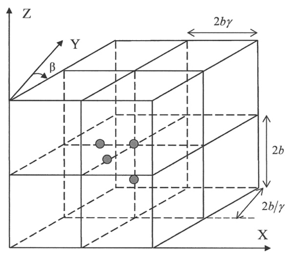
Figure 1 Regular mesh of twenty nodes hexahedral elements and unit cell with four nodes.

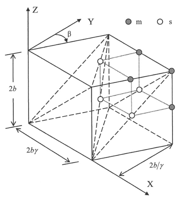
Figure 2 Regular mesh of ten nodes tetrahedral elements and unit cell with four master nodes (m) and four slave nodes (s).

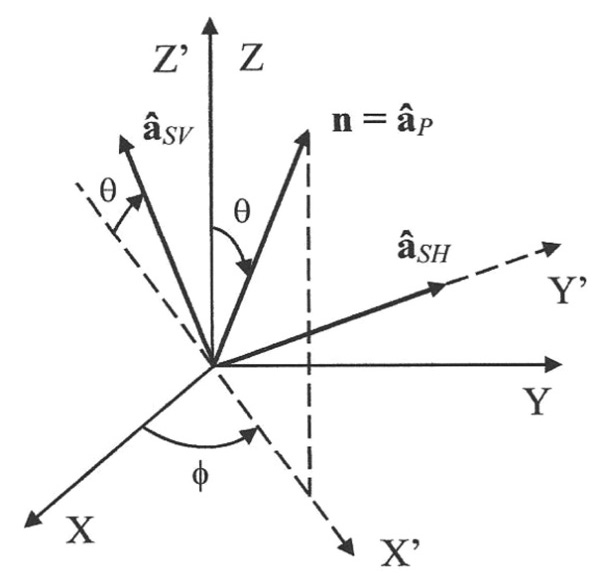
Figure 3 Wave normal and polarization vectors.

where: ũ (r), complex amplitude of the wave; A, amplitude of the wave; $\stackrel{^<!--\; ^\; -->}{\mathbf{a}}$, polarization vector, unit vector indicating the direction of the particle displacement; n, wave normal, unit vector indicating the direction of the wave propagation; κ = 2π/λ = ω/c, wave number; λ, wavelength; c, phase speed of the continuum.

The wave normal has the components

$$\mathbf{n}=(\cos <!--\; \; -->\mathrm{\varphi <!--\; \varphi \; -->}\sin <!--\; \; -->\mathrm{\theta <!--\; \theta \; -->},\sin <!--\; \; -->\mathrm{\varphi <!--\; \varphi \; -->}\sin <!--\; \; -->\mathrm{\theta <!--\; \theta \; -->},\cos <!--\; \; -->\mathrm{\theta <!--\; \theta \; -->})$$

(20)

where: ϕ, azimuthal angle, 0 ≤ ϕ ≤ 180^◦; θ, polar angle, 0 ≤ θ ≤ 180^◦, Figure 3.

For the longitudinal (P) waves the polarization vector will be $\stackrel{^<!--\; ^\; -->}{\mathbf{a}}$ P = n. Two different polarizations $\stackrel{^<!--\; ^\; -->}{\mathbf{a}}$ · n = 0 will be considered for the transverse (S) waves, Figure 3: SV-waves,

$${\stackrel{^<!--\; ^\; -->}{\mathbf{a}}}_{SV}=(-<!--\; -\; -->\cos <!--\; \; -->\mathrm{\varphi <!--\; \varphi \; -->}\cos <!--\; \; -->\mathrm{\theta <!--\; \theta \; -->},-<!--\; -\; -->\sin <!--\; \; -->\mathrm{\varphi <!--\; \varphi \; -->}\cos <!--\; \; -->\mathrm{\theta <!--\; \theta \; -->},\sin <!--\; \; -->\mathrm{\theta <!--\; \theta \; -->})$$

(21)

and SH-waves,

$${\stackrel{^<!--\; ^\; -->}{\mathbf{a}}}_{SH}=(-<!--\; -\; -->\sin <!--\; \; -->\mathrm{\varphi <!--\; \varphi \; -->},\cos <!--\; \; -->\mathrm{\varphi <!--\; \varphi \; -->},0)$$

(22)

For a plane elastic wave Equation (19) the density of period-averaged elastic energy can be computed by the equation [10]

$${\stackrel{¯<!--\; ¯\; -->}{E}}_0=\frac{1}{4}\mathrm{\rho <!--\; \rho \; -->}{\mathrm{\omega <!--\; \omega \; -->}}^2{A}^2$$

(23)

The characteristic equations can be found assuming harmonic waves Equation (19) with different amplitudes in each node of the unit cell,

$$\stackrel{~<!--\; ~\; -->}{\mathbf{u}}=A_j\stackrel{^<!--\; ^\; -->}{\mathbf{a}}\exp <!--\; \; -->(i\mathrm{\kappa <!--\; \kappa \; -->}\mathbf{n}\cdot <!--\; \cdot \; -->\mathbf{r}),j=1,\dots <!--\; \dots \; -->,N$$

(24)

where: N, number of nodes per unit cell.

Inserting the solutions Equation (24) into the homogeneous part of Equation (1), the characteristic equation for each node of the unit cell is yielded by equilibrium of nodal forces into the direction of the particle displacement [11],

$${\mathbf{F}}_K\cdot <!--\; \cdot \; -->\stackrel{^<!--\; ^\; -->}{\mathbf{a}}-<!--\; -\; -->{\mathrm{\omega <!--\; \omega \; -->}}^2{\mathbf{F}}_M\cdot <!--\; \cdot \; -->\stackrel{^<!--\; ^\; -->}{\mathbf{a}}=0$$

(25)

where: FK, nodal force associate to the global stiffness matrix; FM, nodal force associate to the global mass matrix.

By considering Equation (25) for each node of the unit cell, a homogeneous system of N algebraic equations is formed,

$\begin{array}{c}\mathbf{Z}\mathbf{A}=\mathbf{0}\\ z_{ij}{A}_j=0,i,j=1,\dots <!--\; \dots \; -->,N\end{array}$

(26)

$\begin{array}{c}{z}_{ij}=a_{ij}(m,\mathrm{\varphi <!--\; \varphi \; -->},\mathrm{\theta <!--\; \theta \; -->},\mathrm{\nu <!--\; \nu \; -->},\mathrm{\gamma <!--\; \gamma \; -->},\mathrm{\beta <!--\; \beta \; -->})+{\mathrm{\varpi <!--\; \varpi \; -->}}^2{b}_{ij}(m,\mathrm{\varphi <!--\; \varphi \; -->},\mathrm{\theta <!--\; \theta \; -->},\mathrm{\gamma <!--\; \gamma \; -->},\mathrm{\beta <!--\; \beta \; -->})\end{array}$

(27)

$m=b\mathrm{\kappa <!--\; \kappa \; -->}/\mathrm{\pi <!--\; \pi \; -->}=2b/\mathrm{\lambda <!--\; \lambda \; -->},\mathrm{\varpi <!--\; \varpi \; -->}=(2b/c)\mathrm{\omega <!--\; \omega \; -->}$

(28)

where: m, dimensionless wave number, 0 < m < 1; b, half of the element size; ϖ, dimensionless frequency of the discretized elastic domain.

In this procedure, by considering Equation (14) for P-waves and Equation (15) for S-waves, the global stiffness matrix has been expressed in the suitable form

$$\mathbf{K}=\mathrm{\rho <!--\; \rho \; -->}{c}^2(2b){\mathbf{K}}^0$$

(29)

Similarly, the global mass matrix has been suitably expressed as

$$\mathbf{M}=\mathrm{\rho <!--\; \rho \; -->}(2b{)}^3{\mathbf{M}}^0$$

(30)

2.2 Dispersion Equations

The system of homogeneous algebraic equations given in Equation (26) has a non-trivial solution only if the matrix Z is singular; that is, det [Z]= 0. Then it is yielded the following polynomial equation which is called the characteristic frequency equation for the plane wave propagation,

$$\underset{r=0}{\overset{N}{\sum <!--\; \sum \; -->}}{c}_r(m,\mathrm{\varphi <!--\; \varphi \; -->},\mathrm{\theta <!--\; \theta \; -->},\mathrm{\nu <!--\; \nu \; -->},\mathrm{\gamma <!--\; \gamma \; -->},\mathrm{\beta <!--\; \beta \; -->}){\mathrm{\varpi <!--\; \varpi \; -->}}^{2r}=0,c_N=1$$

(31)

It is an important fact that the N zeroes of a polynomial of degree N ≥ 1 with complex coefficients depend continuously upon the coefficients [12]. Thus, sufficiently small changes in the coefficients of a polynomial can lead only to small changes in any zero. However, if the zeros are numerically computed, there is no simple way to define a function which takes the N coefficients (all but the leading 1) of a monic polynomial of degree N to the N zeroes of the polynomial, since there is no natural way to define an ordering among the N zeroes. In the case of the HE20 mesh, for which the polynomial Equation (31) is quartic, the above difficulty has been overcome by computing the zeroes in closed form as functions of its coefficients. Then, the components

$${\mathrm{\varpi <!--\; \varpi \; -->}}_k={\mathrm{\varpi <!--\; \varpi \; -->}}_k(m,\mathrm{\varphi <!--\; \varphi \; -->},\mathrm{\theta <!--\; \theta \; -->},\mathrm{\nu <!--\; \nu \; -->},\mathrm{\gamma <!--\; \gamma \; -->},\mathrm{\beta <!--\; \beta \; -->}),k=1,\dots <!--\; \dots \; -->,4$$

(32)

will be continuous functions precisely defined. They are called the dispersion equations. Substituting Equation (32) into Equation (26), the wave amplitudes corresponding to the nodes of the unit cell for the HE20 mesh are yielded for each dispersion equation.

To find the zeros of a polynomial equation as functions of its coefficients beyond the quartic equation is a very difficult mathematical problem [13]. Then, for the mesh TE10 which has eight nodes per unit cell, if the zeros of Equation (31) are numerically computed, the above mentioned ordering difficulty could be a problem. In this case, by considering the initial condition,

$$\underset{m\to <!--\; \to \; -->0}{lim}{\mathrm{\varpi <!--\; \varpi \; -->}}_1(m,\mathrm{\varphi <!--\; \varphi \; -->},\mathrm{\theta <!--\; \theta \; -->},\mathrm{\nu <!--\; \nu \; -->},\mathrm{\gamma <!--\; \gamma \; -->},\mathrm{\beta <!--\; \beta \; -->})=0$$

(33)

it is proposed to compute the first dispersion equation by a reduced unit cell obtained by a procedure of exact dynamic condensation [14].

Assume that the total nodes at the unit cell are categorized as master nodes (m) and slave nodes (s), where the number of master nodes is four and the number of slave nodes is also four, Figure 2. With this arrangement, the system of characteristic equations Equation (26) may be partitioned as

$$\left(\begin{array}{cc}{\mathbf{Z}}_{mm}& {\mathbf{Z}}_{ms}\\ {\mathbf{Z}}_{sm}& {\mathbf{Z}}_{ss}\end{array}\right)\left(\begin{array}{c}{\mathbf{A}}_m\\ {\mathbf{A}}_s\end{array}\right)=\left(\begin{array}{c}\mathbf{0}\\ \mathbf{0}\end{array}\right)$$

(34)

where:

$$\begin{array}{cc}{\mathbf{Z}}_{mm}={\mathbf{a}}_{mm}+q{\mathbf{b}}_{mm},& {\mathbf{Z}}_{ms}={\mathbf{a}}_{ms}+q{\mathbf{b}}_{ms}\\ {\mathbf{Z}}_{sm}={\mathbf{a}}_{sm}+q{\mathbf{b}}_{sm},& {\mathbf{Z}}_{ss}={\mathbf{a}}_{ss}+q{\mathbf{b}}_{ss}\end{array},q={\mathrm{\varpi <!--\; \varpi \; -->}}^2$$

(35)

The relation of wave amplitudes between the master and slave nodes may be obtained from Equation (34) as

$${\mathbf{A}}_s=-<!--\; -\; -->{\mathbf{Z}}_{ss}^{-<!--\; -\; -->1}(q){\mathbf{Z}}_{sm}(q){\mathbf{A}}_m$$

(36)

Then, by back-substituting, the system of characteristic equations of the reduced unit cell is obtained as

$$\begin{array}{c}{\mathbf{Z}}_R(q){\mathbf{A}}_m=\mathbf{0}\\ [{\mathbf{K}}_R(q)+q{\mathbf{M}}_R(q)]{\mathbf{A}}_m=\mathbf{0}\end{array}$$

(37)

where:

$$\begin{array}{c}{\mathbf{K}}_R(q)={\mathbf{a}}_{mm}-<!--\; -\; -->{\mathbf{Z}}_{ms}{\mathbf{Z}}_{ss}^{-<!--\; -\; -->1}{\mathbf{a}}_{sm}+{\mathbf{Z}}_{ms}{\mathbf{Z}}_{ss}^{-<!--\; -\; -->1}{\mathbf{a}}_{ss}{\mathbf{Z}}_{ss}^{-<!--\; -\; -->1}{\mathbf{Z}}_{sm}-<!--\; -\; -->{\mathbf{a}}_{ms}{\mathbf{Z}}_{ss}^{-<!--\; -\; -->1}{\mathbf{Z}}_{sm}\\ {\mathbf{M}}_R(q)={\mathbf{b}}_{mm}-<!--\; -\; -->{\mathbf{Z}}_{ms}{\mathbf{Z}}_{ss}^{-<!--\; -\; -->1}{\mathbf{b}}_{sm}+{\mathbf{Z}}_{ms}{\mathbf{Z}}_{ss}^{-<!--\; -\; -->1}{\mathbf{b}}_{ss}{\mathbf{Z}}_{ss}^{-<!--\; -\; -->1}{\mathbf{Z}}_{sm}-<!--\; -\; -->{\mathbf{b}}_{ms}{\mathbf{Z}}_{ss}^{-<!--\; -\; -->1}{\mathbf{Z}}_{sm}\end{array}$$

(38)

Then, from Equation (37), the reduced form of the characteristic frequency equation is obtained

$$\begin{array}{c}{q}^4+c_{3R}{q}^3+c_{2R}{q}^2+c_{1R}q+c_{0R}=0\\ c_{rR}(m,\mathrm{\varphi <!--\; \varphi \; -->},\mathrm{\theta <!--\; \theta \; -->},\mathrm{\nu <!--\; \nu \; -->},\mathrm{\gamma <!--\; \gamma \; -->},\mathrm{\beta <!--\; \beta \; -->},q),r=0,\dots <!--\; \dots \; -->,3\end{array}$$

(39)

The first dispersion equation is computed by the following iterative procedure:

Set by Equation (33) the initial value q_i1 = 0.

Do for 0 < m < 1, step Δ m

1. Compute the coefficients c_rR (m, ϕ, θ, ν, γ, β, qi1) of Equation (39).
2. Compute the zero q₁ of the quartic polynomial Equation (39).

Do while (| (q₁ - q_i1)/q1|≥Δ)

1. Refresh initial value q_i1 = q₁.
2. Compute the coefficients c_rR(m, ϕ, θ, ν, γ, β, q_i1) of Equation (39).
3. Compute the zero q₁ of the quartic polynomial Equation (39).

End do

3. Substituting q₁ into Equation (37) to compute the wave amplitudes at the master nodes.
4. Substituting q₁ into Equation (36) to compute the wave amplitudes at the slave nodes.
5. Refresh initial value q_i1 = q₁ for the next step.

End do

The range of dimensionless wave number values where each dispersion equation represents the propagation of elastic waves in the discretized medium will be called the acoustical branch of the dispersion equation. In order to determine the acoustical branches, a preliminary constraint condition over the dimension of the null space of Z for the HE20 mesh, or ZR for the TE10 mesh, must be imposed,

$$\dim <!--\; \; -->[\mathbf{N}(\mathbf{Z})]=1\mathit{o}\mathit{r}\dim <!--\; \; -->[\mathbf{N}({\mathbf{Z}}_R)]=1$$

(40)

The constraint condition Equation (40) implies that the subspace of solutions to Equation (25) or Equation (37) must be one-dimensional. In this case the vector of wave amplitudes A or A_m is arbitrary to the extent that a scalar multiple of it is also a solution. Then the following constraint conditions are imposed,

$A_1=1;A_j(m,\mathrm{\varphi <!--\; \varphi \; -->},\mathrm{\theta <!--\; \theta \; -->},\mathrm{\nu <!--\; \nu \; -->},\mathrm{\gamma <!--\; \gamma \; -->},\mathrm{\beta <!--\; \beta \; -->})>0,j=2,3,4$	(41)
$(\mathrm{\partial <!--\; \partial \; -->}\mathrm{\varpi <!--\; \varpi \; -->}/\mathrm{\partial <!--\; \partial \; -->}m{)}_{\mathrm{\varphi <!--\; \varphi \; -->},\mathrm{\theta <!--\; \theta \; -->},\mathrm{\nu <!--\; \nu \; -->},\mathrm{\gamma <!--\; \gamma \; -->},\mathrm{\beta <!--\; \beta \; -->}}>0$	(42)

In molecular physics, condition Equation (41) is called the restriction of the lattice spectrum to the acoustical branch [15]. Obviously, if the constraint condition Equation (40) is not imposed, the constraint condition Equation (41) is meaningless.

From Equation (28) we obtain both the phase velocity and group velocity of the discretized medium,

$c_d=c(2\mathrm{\pi <!--\; \pi \; -->}{)}^{-<!--\; -\; -->1}\mathrm{\varpi <!--\; \varpi \; -->}/m$	(43)
$c_{g,d}=\mathrm{\partial <!--\; \partial \; -->}\mathrm{\omega <!--\; \omega \; -->}/\mathrm{\partial <!--\; \partial \; -->}\mathrm{\kappa <!--\; \kappa \; -->}=c_g(2\mathrm{\pi <!--\; \pi \; -->}{)}^{-<!--\; -\; -->1}\mathrm{\partial <!--\; \partial \; -->}\mathrm{\varpi <!--\; \varpi \; -->}/\mathrm{\partial <!--\; \partial \; -->}m$	(44)

where: c_g, group velocity of the continuum.

From Equation (44), the constraint condition Equation (42) is equivalent to

$$c_{g,d}>0$$

(45)

It can be proven that for general periodic motion the energy propagates with the group velocity [2]; therefore, the constraint condition Equation (45) imposes that the energy propagates into the wave direction. From this point, for each dispersion equation only the acoustical branch will be considered. This one represents the physically admissible solution for mechanical wave propagation.

It must be recall that the group velocity of the continuum will be equal to the phase velocity because the waves propagate non-dispersively. Nevertheless, for the dispersive discretized medium the group velocity will be different from the phase velocity; therefore, the velocity of energy transport will be different from the phase velocity. As a consequence, when the numerical dispersion associated with the finite element spatial discretization is considered, not only the effect over the phase velocity must be analyzed but also the effect over the group velocity or velocity of energy transport.

By considering Equations (43) and (44), the indicators of the dispersion associated with the spatial discretization that is introduced by the finite element model are defined as

$\begin{array}{rl}{e}_p& =c_d/c=(2\mathrm{\pi <!--\; \pi \; -->}{)}^{-<!--\; -\; -->1}\mathrm{\varpi <!--\; \varpi \; -->}/m,e_p=e_p(m,\mathrm{\varphi <!--\; \varphi \; -->},\mathrm{\theta <!--\; \theta \; -->},\mathrm{\nu <!--\; \nu \; -->},\mathrm{\gamma <!--\; \gamma \; -->},\mathrm{\beta <!--\; \beta \; -->})\end{array}$

(46)

$\begin{array}{rl}{e}_g& =c_{g,d}/c_g=(2\mathrm{\pi <!--\; \pi \; -->}{)}^{-<!--\; -\; -->1}\mathrm{\partial <!--\; \partial \; -->}\mathrm{\varpi <!--\; \varpi \; -->}/\mathrm{\partial <!--\; \partial \; -->}m,e_g=e_g(m,\mathrm{\varphi <!--\; \varphi \; -->},\mathrm{\theta <!--\; \theta \; -->},\mathrm{\nu <!--\; \nu \; -->},\mathrm{\gamma <!--\; \gamma \; -->},\mathrm{\beta <!--\; \beta \; -->})\end{array}$

(47)

These indicators consider the effect of the spatial discretization on the wave velocity and the velocity of energy transport, respectively.

2.3 Elastic Energy at the Unit Cell

From Equations (2), (28) and (29) the elastic energy at the unit cell over a period will be

$$E=\frac{1}{2}\mathrm{\rho <!--\; \rho \; -->}(\mathrm{\omega <!--\; \omega \; -->}/\mathrm{\varpi <!--\; \varpi \; -->}{)}^2(2b{)}^3\mathrm{R}\mathrm{e}[{\stackrel{~<!--\; ~\; -->}{\mathbf{x}}}^t\exp <!--\; \; -->(-<!--\; -\; -->i2\mathrm{\pi <!--\; \pi \; -->}\mathrm{\tau <!--\; \tau \; -->})]\mathrm{R}\mathrm{e}[{\stackrel{~<!--\; ~\; -->}{\mathbf{F}}}^0\exp <!--\; \; -->(-<!--\; -\; -->i2\mathrm{\pi <!--\; \pi \; -->}\mathrm{\tau <!--\; \tau \; -->})]$$

(48)

where: ${\mathbf{F}}^0={\stackrel{~<!--\; ~\; -->}{\mathbf{F}}}^0\exp <!--\; \; -->(-<!--\; -\; -->i2\mathrm{\pi <!--\; \pi \; -->}\mathrm{\tau <!--\; \tau \; -->})$, column matrix of forces at the nodes of the unit cell, obtained from the stiffness matrix K⁰ defined in Equation (29).

From Equation (48), the density of period-averaged elastic energy is computed,

$$\stackrel{¯<!--\; ¯\; -->}{E}=\frac{1}{2}\mathrm{\rho <!--\; \rho \; -->}(\mathrm{\omega <!--\; \omega \; -->}/\mathrm{\varpi <!--\; \varpi \; -->}{)}^2{\int <!--\; \int \; -->}_0^1\mathrm{R}\mathrm{e}[{\stackrel{~<!--\; ~\; -->}{\mathbf{x}}}^t\exp <!--\; \; -->(-<!--\; -\; -->i2\mathrm{\pi <!--\; \pi \; -->}\mathrm{\tau <!--\; \tau \; -->})]\mathrm{R}\mathrm{e}[{\stackrel{~<!--\; ~\; -->}{\mathbf{F}}}^0\exp <!--\; \; -->(-<!--\; -\; -->i2\mathrm{\pi <!--\; \pi \; -->}\mathrm{\tau <!--\; \tau \; -->})]d\mathrm{\tau <!--\; \tau \; -->}$$

(49)

From the decomposition in Equation (7), the above density of period-averaged elastic energy Equation (49) can be partitioned as addition of basic and higher order components. The latter component will be

$${\stackrel{¯<!--\; ¯\; -->}{E}}_h=\frac{1}{2}\mathrm{\rho <!--\; \rho \; -->}(\mathrm{\omega <!--\; \omega \; -->}/\mathrm{\varpi <!--\; \varpi \; -->}{)}^2{\int <!--\; \int \; -->}_0^1\mathrm{R}\mathrm{e}[{\stackrel{~<!--\; ~\; -->}{\mathbf{x}}}^t\exp <!--\; \; -->(-<!--\; -\; -->i2\mathrm{\pi <!--\; \pi \; -->}\mathrm{\tau <!--\; \tau \; -->})]\mathrm{R}\mathrm{e}[{\stackrel{~<!--\; ~\; -->}{\mathbf{F}}}_h^0\exp <!--\; \; -->(-<!--\; -\; -->i2\mathrm{\pi <!--\; \pi \; -->}\mathrm{\tau <!--\; \tau \; -->})]d\mathrm{\tau <!--\; \tau \; -->}$$

(50)

From Equations (50) and (49), the percentage of period-averaged higher order elastic energy can be defined as

$$e_h={\stackrel{¯<!--\; ¯\; -->}{E}}_h/\stackrel{¯<!--\; ¯\; -->}{E},e_h=e_h(m,\mathrm{\varphi <!--\; \varphi \; -->},\mathrm{\theta <!--\; \theta \; -->},\mathrm{\nu <!--\; \nu \; -->},\mathrm{\gamma <!--\; \gamma \; -->},\mathrm{\beta <!--\; \beta \; -->})$$

(51)

From Equations (49) and (23), the percentage indicator of elastic energy error associated with the spatial discretization that is introduced bythe finite element model is defined as

$$\mathrm{\epsilon <!--\; \epsilon \; -->}=(\stackrel{¯<!--\; ¯\; -->}{E}/{\stackrel{¯<!--\; ¯\; -->}{E}}_0)-<!--\; -\; -->1,\mathrm{\epsilon <!--\; \epsilon \; -->}=\mathrm{\epsilon <!--\; \epsilon \; -->}(m,\mathrm{\varphi <!--\; \varphi \; -->},\mathrm{\theta <!--\; \theta \; -->},\mathrm{\nu <!--\; \nu \; -->},\mathrm{\gamma <!--\; \gamma \; -->},\mathrm{\beta <!--\; \beta \; -->})$$

(52)

2.4 Numerical Research

Three different meshes having the same element volume will be considered for each of the elements analyzed. Specifically, Figures 1 and 2:

Q1: square section; γ = 1, β = 0.

Q2: rectangular section with aspect ratio 1:2; $\mathrm{\gamma <!--\; \gamma \; -->}=1/\surd <!--\; \surd \; -->2$, β = 0.

Q3: skewed section; γ = 1, β = 45^◦.

Given the mesh and the Poisson’s ratio, the dispersion analysis is numerically carried out by a step of π/36 for the azimuthal and polar angles, and a step of 1/10000 for the dimensionless wave number. As result the indicators Equations (46), (47), (51) and (52), are computed as finite sets of values.

For the mesh HE20-Q1 and SV-waves the indicators Equations (52) and (51) are plotted versus dimensionless wave number, Figures 4 and 5, for three directions of wave propagation. It is observed both indicators vanish as dimensionless wave number goes to zero; that is, as the mesh is refined and in the limit of long waves. Then, a mapping between the elastic energy error Equation (52) and the percentage of higher order elastic energy Equation (51) could be computed,

$$\mathrm{\epsilon <!--\; \epsilon \; -->}=\mathrm{\epsilon <!--\; \epsilon \; -->}(e_h,\mathrm{\varphi <!--\; \varphi \; -->},\mathrm{\theta <!--\; \theta \; -->},\mathrm{\nu <!--\; \nu \; -->},\mathrm{\gamma <!--\; \gamma \; -->},\mathrm{\beta <!--\; \beta \; -->})$$

(53)

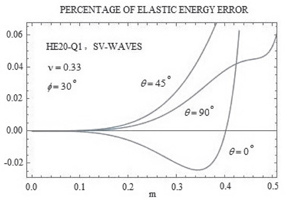
Figure 4 Indicator of elastic energy error versus dimensionless wave number.

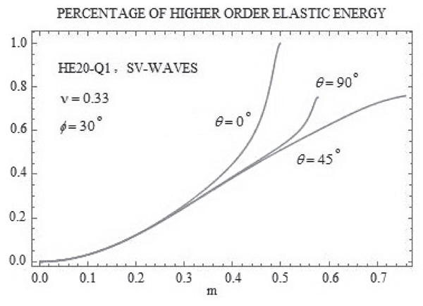
Figure 5 Percentage of higher order elastic energy versus dimensionless wave number.

It must be remarked that the behavior of the higher order elastic energy as dimensionless wave number goes to zero is a consequence that the strain field inside each element becomes uniform. That is, given the mesh, in the limit of long waves, the density of elastic energy approaches to zero more slowly than its higher order component; and, given the wavelength, as the solution converges on account of mesh refinement, the density of elastic energy is increasingly dominated by its basic component.

For the mesh HE20-Q1 and SV-waves, the mapping Equation (53) is plotted in Figure 6 for three directions of wave propagation. Similarly, for the mesh TE10-Q1 and SV-waves the mapping Equation (53) is plotted in Figure 7 for four directions of wave propagation. In both cases it is observed that, for moderate values of percentage of higher order elastic energy, this mapping could be approximated by the following cubic correlation,

$$\mathrm{\epsilon <!--\; \epsilon \; -->}=[A(\mathrm{\varphi <!--\; \varphi \; -->},\mathrm{\theta <!--\; \theta \; -->},\mathrm{\nu <!--\; \nu \; -->},\mathrm{\gamma <!--\; \gamma \; -->},\mathrm{\beta <!--\; \beta \; -->})\ast <!--\; \ast \; -->e_h+B(\mathrm{\varphi <!--\; \varphi \; -->},\mathrm{\theta <!--\; \theta \; -->},\mathrm{\nu <!--\; \nu \; -->},\mathrm{\gamma <!--\; \gamma \; -->},\mathrm{\beta <!--\; \beta \; -->})]\ast <!--\; \ast \; -->e_h^2$$

(54)

In this paper an averaged correlation between the elastic energy error and the percentage of higher order elastic energy with the Poisson’s ratio as parameter is sought by computing averaged values for the coefficients A and B.

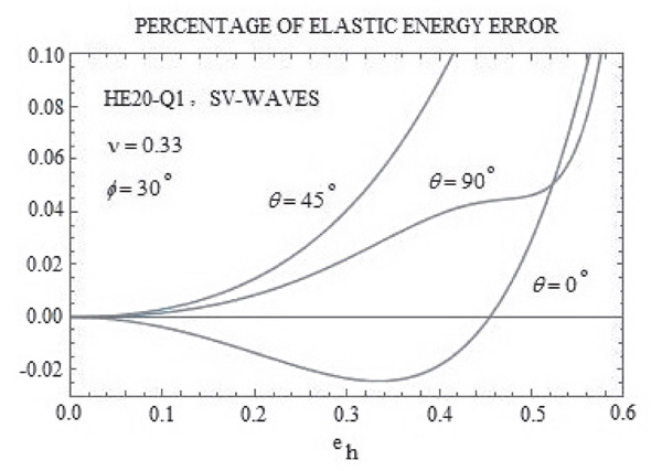
Figure 6 Percentage of elastic energy error versus percentage of higher order elastic energy for HE20 element.

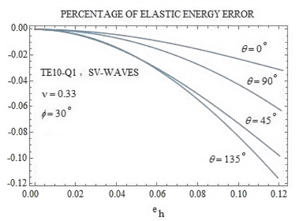
Figure 7 Percentage of elastic energy error versus percentage of higher order elastic energy for TE10 element.

First, two values of percentage of higher order elastic energy Equation (51) are selected as reference ones, for each of the elements considered,

$$\begin{gathered} e_{h1}^{HE20}=0.10e_{h2}^{HE20}=0.20 \\ {e}_{h1}^{TE10}=0.03e_{h2}^{TE10}=0.06 \end{gathered}$$

(55)

Then, by Equations (51) and (53), the related reference values of dimensionless wave number and percentage of elastic energy error are respectively computed,

$\begin{array}{rl}{m}_{1,2}& =f_{m1,2}(\mathrm{\varphi <!--\; \varphi \; -->},\mathrm{\theta <!--\; \theta \; -->},\mathrm{\nu <!--\; \nu \; -->},\mathrm{\gamma <!--\; \gamma \; -->},\mathrm{\beta <!--\; \beta \; -->})\end{array}$	(56)
$$\begin{array}{rl}{\mathrm{\epsilon <!--\; \epsilon \; -->}}_{1,2}& =f_{\mathrm{\epsilon <!--\; \epsilon \; -->}1,2}(\mathrm{\varphi <!--\; \varphi \; -->},\mathrm{\theta <!--\; \theta \; -->},\mathrm{\nu <!--\; \nu \; -->},\mathrm{\gamma <!--\; \gamma \; -->},\mathrm{\beta <!--\; \beta \; -->})\end{array}$$	(57)

where: |ɛ₁| = |ɛ(m)|_max,m∈ (0,m₁] and |ɛ₂| = |ɛ(m)|_max,m ∈ (0,m₂]. Next, the mean value of each reference dimensionless wave number and the root-mean-square value of each reference elastic energy error are computed on the range of propagation angle,

$$\begin{array}{rl}{m}_{1,2}^M(\mathrm{\nu <!--\; \nu \; -->},\mathrm{\gamma <!--\; \gamma \; -->},\mathrm{\beta <!--\; \beta \; -->})& =\frac{1}{{\mathrm{\pi <!--\; \pi \; -->}}^2}{\int <!--\; \int \; -->}_0^{\mathrm{\pi <!--\; \pi \; -->}}{\int <!--\; \int \; -->}_0^{\mathrm{\pi <!--\; \pi \; -->}}{m}_{1,2}d\mathrm{\varphi <!--\; \varphi \; -->}d\mathrm{\theta <!--\; \theta \; -->}\end{array}$$

(58)

$$\begin{array}{rl}{\mathrm{\epsilon <!--\; \epsilon \; -->}}_{1,2}^{RMS}(\mathrm{\nu <!--\; \nu \; -->},\mathrm{\gamma <!--\; \gamma \; -->},\mathrm{\beta <!--\; \beta \; -->})& =\sqrt{\frac{1}{{\mathrm{\pi <!--\; \pi \; -->}}^2}{\int <!--\; \int \; -->}_0^{\mathrm{\pi <!--\; \pi \; -->}}{\int <!--\; \int \; -->}_0^{\mathrm{\pi <!--\; \pi \; -->}}{\mathrm{\epsilon <!--\; \epsilon \; -->}}_{1,2}^{2}d\mathrm{\varphi <!--\; \varphi \; -->}d\mathrm{\theta <!--\; \theta \; -->}}\end{array}$$

(59)

Consistent with the discrete analysis carried out, the integrals in Equations (58) and (59) are numerically computed by the classical Trapezoidal rule. By similar procedure, mean reference values of the indicators of numerical dispersion for the phase velocity Equation (46) and the group velocity Equation (47) are also computed. Detailed values are presented in the Appendix attached to this manuscript.

In Tables A3 and A4, the mesh averaging of the root-mean-square values of the first and second reference percentage of elastic energy error Equation (59) are computed versus the Poisson’s ratio,

$$\stackrel{¯<!--\; ¯\; -->}{{\mathrm{\epsilon <!--\; \epsilon \; -->}}_{1,2}^{RMS}}(\mathrm{\nu <!--\; \nu \; -->})=\frac{1}{3}[{\mathrm{\epsilon <!--\; \epsilon \; -->}}_{1,2}^{RMS}(\mathrm{\nu <!--\; \nu \; -->},Q_1)+{\mathrm{\epsilon <!--\; \epsilon \; -->}}_{1,2}^{RMS}(\mathrm{\nu <!--\; \nu \; -->},Q_2)+{\mathrm{\epsilon <!--\; \epsilon \; -->}}_{1,2}^{RMS}(\mathrm{\nu <!--\; \nu \; -->},Q_3)]$$

(60)

The values for S-waves are obtained by considering both SV-waves and SH- waves. By linear interpolation, the above mesh-averaged values can also be computed for other values of Poisson’s ratio. By similar procedure, the mesh averaging of the mean values of the first and second reference dimensionless wave number have been computed versus the Poisson’s ratio in Tables A1 and A2. The mesh averaging of the mean values of the second reference value for the indicators of dispersion associated with the phase and group velocities have been also computed in Tables A5 and A6.

Finally, by the mesh-averaged reference values of elastic energy error Equation (60), the averaged values of the coefficients A and B for the cubic correlation Equation (54) are then computed versus the Poisson’s ratio,

$$\left(\begin{array}{c}A(\mathrm{\nu <!--\; \nu \; -->})\\ B(\mathrm{\nu <!--\; \nu \; -->})\end{array}\right)={\left(\begin{array}{cc}{e}_{h1}^3& e_{h1}^2\\ e_{h2}^3& e_{h2}^2\end{array}\right)}^{-<!--\; -\; -->1}\left(\begin{array}{c}\stackrel{¯<!--\; ¯\; -->}{{\mathrm{\epsilon <!--\; \epsilon \; -->}}_1^{RMS}}(\mathrm{\nu <!--\; \nu \; -->})\\ \stackrel{¯<!--\; ¯\; -->}{{\mathrm{\epsilon <!--\; \epsilon \; -->}}_2^{RMS}}(\mathrm{\nu <!--\; \nu \; -->})\end{array}\right)$$

(61)

By considering Equations (61) and (55), the P and S averaged correlations are obtained, both for the twenty nodes hexahedral element HE20 and for the ten nodes tetrahedral element TE10,

$\begin{array}{rl}{\mathrm{\epsilon <!--\; \epsilon \; -->}}_{P,S}^{HE20}& =[A_{P,S}^{HE20}(\mathrm{\nu <!--\; \nu \; -->})\ast <!--\; \ast \; -->e_h+B_{P,S}^{HE20}(\mathrm{\nu <!--\; \nu \; -->})]\ast <!--\; \ast \; -->e_h^2,0<e_h\le <!--\; \le \; -->e_{h2}^{HE20}\end{array}$	(62)
$$\begin{array}{rl}{\mathrm{\epsilon <!--\; \epsilon \; -->}}_{P,S}^{TE10}& =[A_{P,S}^{TE10}(\mathrm{\nu <!--\; \nu \; -->})\ast <!--\; \ast \; -->e_h+B_{P,S}^{TE10}(\mathrm{\nu <!--\; \nu \; -->})]\ast <!--\; \ast \; -->e_h^2,0<e_h\le <!--\; \le \; -->e_{h2}^{TE10}\end{array}$$	(63)

From Tables A3 and A4, the following inequalities can be deduced, both for the twenty nodes hexahedral element HE20 and the ten nodes tetrahedral element TE10,

$${\mathrm{\epsilon <!--\; \epsilon \; -->}}_P(e_h,{\mathrm{\nu <!--\; \nu \; -->}}_a)>{\mathrm{\epsilon <!--\; \epsilon \; -->}}_S(e_h,{\mathrm{\nu <!--\; \nu \; -->}}_a),0.05\le <!--\; \le \; -->{\mathrm{\nu <!--\; \nu \; -->}}_a\le <!--\; \le \; -->0.45$$

(64)

$$\begin{gathered} \mathrm{\Delta <!--\; \Delta \; -->}\mathrm{\epsilon <!--\; \epsilon \; -->}(e_h,{\mathrm{\nu <!--\; \nu \; -->}}_a)<\mathrm{\Delta <!--\; \Delta \; -->}\mathrm{\epsilon <!--\; \epsilon \; -->}(e_h,{\mathrm{\nu <!--\; \nu \; -->}}_b),0.05\le <!--\; \le \; -->{\mathrm{\nu <!--\; \nu \; -->}}_a<{\mathrm{\nu <!--\; \nu \; -->}}_b\le <!--\; \le \; -->0.45 \\ \mathrm{\Delta <!--\; \Delta \; -->}\mathrm{\epsilon <!--\; \epsilon \; -->}={\mathrm{\epsilon <!--\; \epsilon \; -->}}_P-<!--\; -\; -->{\mathrm{\epsilon <!--\; \epsilon \; -->}}_S \end{gathered}$$

(65)

From the mesh-averaged reference values in Tables A1 and A2, it can be deduced that the second reference value of percentage of higher order elastic energy, Equation (55), upper bounding the range of the P and S averaged correlations, Equations (62) and (63), roughly corresponds, in an averaged sense, to four and five elements per wavelength for the HE20 and TE10 elements, respectively. Similarly, the first reference value roughly corresponds, in an averaged sense, to six and seven elements per wavelength for the HE20 and TE10 elements, respectively. As a consequence, from the mesh- averaged reference values in Tables A3 and A4, it can be deduced that the TE10 mesh, despite having one more element per wavelength in an averaged sense, generates an elastic energy error higher than the one generated with the HE20 mesh. The higher performance of the HE20 element, from the elastic energy error standpoint, is clearly displayed. This behavior is related to the element internal degrees of freedom [16]. Both elements have 6 rigid body modes, 6 constant strain states and 18 linear strain states (the complete set of linear strain states); however, the HE20 element additionally has 21 quadratic strain states (30 needed for completeness) and 9 cubic strain states (42 needed for completeness).

2.5 Substitute Wave Field

It is clear that the harmonic elastic waves cannot be exactly captured by a regular mesh of finite elements HE20 or TE10. This fact is a consequence of the element interpolation which is quadratic. A substitute wave field [17] or alias field [16] has been obtained in the discretized unbounded medium by performing a dispersion analysis in terms of allowable polarizations of the continuum. The substitute wave field is obtained by collocating Equation (24) in each node of the unit cell. The assumption of different amplitudes is introduced because the equation of equilibrium is different for each node. The analysis yields the relative wave amplitudes and the dispersion relation under which the alias field may propagate in the discretized medium. The alias wave field will be

$${\stackrel{~<!--\; ~\; -->}{\mathbf{u}}}^a=\sum <!--\; \sum \; -->N_{S,i}{\stackrel{~<!--\; ~\; -->}{\mathbf{u}}}_i$$

(66)

where: ū_i, the values of Equation (24) at the nodes; N_S,i, the nodal shape functions.

By computing the wave amplitude distortion, the discretization error of the wave field Equation (66) can be decomposed as addition of interpolation and pollution errors [18].

2.6 Influence of the Poisson’s Ratio

For the longitudinal waves, which are dilatational waves, by considering the constitutive law Equation (10), the denominator in Equation (11) suggests that significant numerical errors in the stresses could be expected when the Poisson’s ratio approaches the one half value, which can happen for the so-called almost incompressible solids, because the Lamé constant λ increases indefinitely. The very small volumetric strain, approaching zero in the limit of total incompressibility, is determined from derivatives of displacements, which are not as accurately predicted as the displacements themselves. Any error in the predicted volumetric strain will appear as a large error in the stresses, and this error will in turn significantly increases the elastic energy error [7, 16]. Similarly, for the transverse waves, which are rotational waves, the alias wave field Equation (66), which has different amplitude in each node of the unit cell, could produce spurious volumetric strain that also would significantly increase the elastic energy error when the Poisson’s ratio approaches the one half value. This behaviour is the well-known dilatational locking and its effect on elastic energy error is clearly observed in the mesh- averaged values displayed in Tables A3 and A4. The volumetric strain error must have a prevailing effect on the elastic energy error, increasing the elastic energy error for the longitudinal waves versus the one for the transverse waves, Equation (64). The difference between them is all the greater as the Poisson’s ratio is greater, in accordance with the inequality Equation (65).

For the longitudinal waves, the system of characteristic Equation (26) is formed by the dimensionless elasticity matrix Equation (16). The non-constant coefficients in this matrix are weakly depended on the Poisson’s ratio, Figure 8. Then, it is expected that the characteristic frequency Equation (31) would be also weakly depended on the Poisson’s ratio and so the dimensionless frequencies computed would be. However, for the transverse waves, the system of characteristic Equation (26) is formed by the dimensionless elasticity matrix Equation (17). The non-constant coefficients in this matrix increase indefinitely when the Poisson’s ratio approaches the one half value, Figure 8. Then, by considering Equation (27), it would be expected a corresponding significant increase in the computed values of the coefficients associated to the global stiffness matrix and therefore a corresponding increase in the computed values of dimensionless frequency. The effect of this behavior on the indicators of dispersion is clearly observed in the mesh-averaged values displayed in Tables A5 and A6. The value of each indicator for the transverse waves is greater than the one for the longitudinal waves and the difference between them is all the greater as the Poisson’s ratio is greater, as it would be expected.

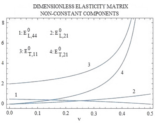
Figure 8 Dimensionless elasticity matrix. Non-constant components versus the Poisson’s ratio.

3 Finite Element Modal Analysis

As application it is explored the use of the averaged correlations Equations (62) and (63) as a reference to apply the higher order elastic energy as an error indicator for the finite element vibration eigenmodes. These ones are the solution of the eigenproblem [7],

$$(\mathbf{K}-<!--\; -\; -->{\mathrm{\omega <!--\; \omega \; -->}}_j^{2}M){\stackrel{~<!--\; ~\; -->}{\mathrm{\psi <!--\; \psi \; -->}}}_j=\mathbf{0},j=1,\dots <!--\; \dots \; -->,n$$

(67)

where ω_j and ${\stackrel{~<!--\; ~\; -->}{\psi <!--\; \psi \; -->}}_j$ are the finite element natural frequencies and eigenvectors, respectively.

By introducing the relation of K-orthogonality

$${\stackrel{~<!--\; ~\; -->}{\mathrm{\psi <!--\; \psi \; -->}}}_i^{T}K{\stackrel{~<!--\; ~\; -->}{\mathrm{\psi <!--\; \psi \; -->}}}_j={\mathrm{\delta <!--\; \delta \; -->}}_{ij}{\mathrm{\omega <!--\; \omega \; -->}}_j^2$$

(68)

into Equation (8), the following expression for the modal elastic energy is yielded,

$${\stackrel{¯<!--\; ¯\; -->}{E}}_j=\frac{1}{4}{\mathrm{\omega <!--\; \omega \; -->}}_j^2,j=1,\dots <!--\; \dots \; -->,n$$

(69)

The error for the modal elastic energy computed with the discretized elastic domain can be estimated by a more precise reference model obtained by mesh halving (that is, by dividing each element of the actual mesh into eight to the nth power elements). The modal elastic energies computed with the actual model and the ones computed with the reference model will be compared by

$$\mathit{\text{EEE}}=(\stackrel{¯<!--\; ¯\; -->}{E}/{\stackrel{¯<!--\; ¯\; -->}{E}}^{\mathit{\text{REF}}})-<!--\; -\; -->1,\mathit{\text{EEE}}=(\mathrm{\omega <!--\; \omega \; -->}/{\mathrm{\omega <!--\; \omega \; -->}}^{\mathit{\text{REF}}}{)}^2-<!--\; -\; -->1$$

(70)

where $\stackrel{¯<!--\; ¯\; -->}{E}$ and ${\stackrel{¯<!--\; ¯\; -->}{E}}^{\mathit{\text{REF}}}$ are defined by Equations (8) and (69) has been taking into account.

The modal elastic energy error computed by mesh halving Equation (70) will be compared with the so-defined as standard modal elastic energy error which is computed by the correlation Equations (62) or (63) for the S-waves,

$$\mathit{\text{SEEEs}}(\mathit{\text{PHE}},\mathrm{\nu <!--\; \nu \; -->})={\mathrm{\epsilon <!--\; \epsilon \; -->}}_S.0<\mathit{\text{PHE}}\le <!--\; \le \; -->e_{h2}$$

(71)

where: PHE, percentage of higher order elastic energy computed with the actual model by Equations (8) and (9), and upper bounded by the second reference value defined in Equation (55).

From the mesh-averaged reference values displayed in Tables A3 and A4, it can be deduced that the standard modal elastic energy error Equation (71) will be weakly dependent on the Poisson’s ratio.

In order to select the standard modal elastic energy error Equation (71), it has been taking into account the heuristic that given the natural frequency both the percentage of higher order elastic energy and the spatial discretization error should be mainly influenced by the slowest S-waves which have the shortest wavelengths.

In order to compare the standard modal elastic energy error Equation (71) with the modal elastic energy error Equation (70), three typical test problems will be analyzed: a pyramidal block fixed at its base discretized by a regular mesh of 512 TE10 elements, Figure 9; a tapered block fixed at its base discretized by a quasi-regular mesh of 128 HE20 elements, Figure 10; and a cantilever beam discretized by a regular mesh of 384 HE20 elements, Figure 11 [19]. The above solids are made of lead, aluminum and steel, respectively.

Since each solid has two planes of symmetry, XY and XZ, the modes have been computed by idealizing one quarter of it and applying four combinations of boundary conditions on the two planes for symmetric motion (S) and for antisymmetric motion (A), see details in reference [19]. The results of the analysis are displayed in Table 1, for the pyramidal block, in Tables 2a and 2b for the tapered block, and in Tables 3a to 3d for the cantilever beam.

In each case the reference model has been obtained by dividing each element of the actual mesh into eight elements. The rate of convergence of the elements TE10 and HE20, both of them have the complete set of linear strain states, and computational cost reasons have been taking into account in this selection.

It is deduced that, for each of the eigenmodes computed, the percentage of higher order energy decreases as the mesh is refined. Then, this energy component behaves as a modal error indicator, which is in accordance with the numerical dispersion analysis.

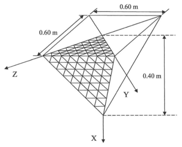
Figure 9 Lead pyramidal block. $\mathrm{E}=17\times <!--\; \times \; -->{10}^{9}Pa;\mathrm{\nu <!--\; \nu \; -->}=0.40;\mathrm{\rho <!--\; \rho \; -->}=11370kg/m{}^3$.

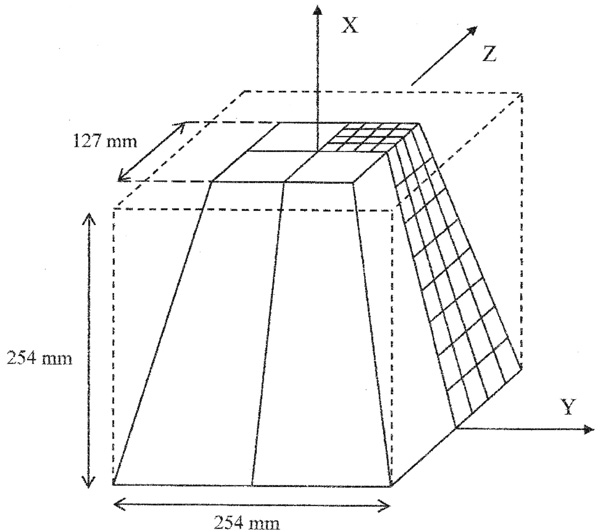
Figure 10 Aluminum tapered block. $\mathrm{E}=72\times <!--\; \times \; -->{10}^{9}Pa;\mathrm{\nu <!--\; \nu \; -->}=0.31;\mathrm{\rho <!--\; \rho \; -->}=2780kg/m{}^3$.

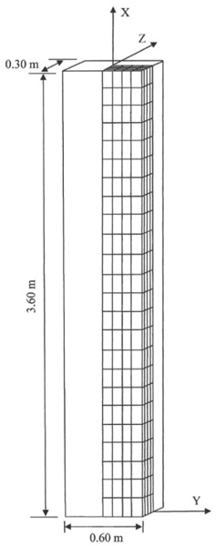
Figure 11 Steel cantilever beam. $\mathrm{E}=206.8\times <!--\; \times \; -->{10}^{9}Pa,\mathrm{\nu <!--\; \nu \; -->}=0.30,\mathrm{\rho <!--\; \rho \; -->}=8058kg/m{}^3$.

Table 1 Lead pyramidal block. Standard modal elastic energy error SEEEs versus modal elastic energy error computed by mesh halving EEE

MODE		FR (Hz)	PHE	EEE	SEEEs	PHE REF
1	SA	786.44	0.007562	0.000626	0.000421	0.002069
2	AA	1096.29	0.022623	0.003175	0.003670	0.006278
3	SS	1331.48	0.015905	0.002075	0.001836	0.004418
4	SA	1352.15	0.036275	0.004688	0.009208	0.010068
5	SS	1701.77	0.027239	0.004879	0.005278	0.007642
6	AA	1786.89	0.027171	0.004356	0.005252	0.007688
7	AA	1858.46	0.059875	0.013884	0.024005	0.017143
8	SA	1914.96	0.047425	0.010629	0.015418	0.013704
9	SA	2117.91	0.040341	0.009748	0.011303	0.012539
10	AA	2157.59	0.051531	0.012201	0.018063	0.014716
11	SA	2159.55	0.065810	0.010680	0.028671	0.018122
12	SS	2168.77	0.053274	0.012092	0.019243	0.015128
13	SA	2318.81	0.063315	0.017092	0.026666	0.018273
14	AA	2339.55	0.059458	0.020168	0.023690	0.017298
15	SS	2377.37	0.056629	0.014164	0.021605	0.016696

FR, natural frequency computed with the actual model; PHE, percentage of higher order elastic energy computed with the actual model; EEE, elastic energy error computed by mesh halving; SEEEs, standard elastic energy error; PHE REF, percentage of higher order elastic energy computed by mesh halving.

Table 2a Aluminum tapered block. Standard modal elastic energy error SEEEs versus modal elastic energy error computed by mesh halving EEE. Modes 1–27

MODE		FR (Hz)	PHE	EEE	SEEEs	PHE REF
1	AS	2878.85	0.018132	0.000813	0.000086	0.005230
2	AA	4552.87	0.040784	0.000478	0.000441	0.010864
3	SS	6381.21	0.010614	0.000488	0.000029	0.003100
4	AS	6735.84	0.038988	0.000759	0.000403	0.010463
5	AA	9357.29	0.069749	0.001114	0.001321	0.018948
6	AA	11530.20	0.048941	0.000648	0.000640	0.013042
7	AS	11817.84	0.059180	0.001504	0.000943	0.016156
8	SS	12271.50	0.047472	0.000801	0.000601	0.012674
9	AA	12326.57	0.052072	0.000475	0.000726	0.013880
10	AS	12539.56	0.061821	0.000784	0.001031	0.016426
11	AS	13175.85	0.072668	0.001792	0.001438	0.020030
12	SS	13885.66	0.054707	0.001123	0.000803	0.014696
13	SS	14009.28	0.064478	0.001346	0.001124	0.017591
14	AA	14602.80	0.125306	0.003293	0.004455	0.035078
15	SS	14692.37	0.101382	0.001081	0.002863	0.027148
16	AA	15463.61	0.098834	0.001468	0.002715	0.026757
17	AS	15701.96	0.085086	0.001344	0.001991	0.022867
18	SS	15991.34	0.097402	0.001555	0.002634	0.026108
19	SS	16207.91	0.070687	0.001305	0.001358	0.018780
20	AA	16680.95	0.060341	0.000827	0.000981	0.016028
21	AS	16789.52	0.109945	0.001763	0.003389	0.030133
22	AS	17512.27	0.104593	0.003809	0.003054	0.029812
23	SS	17590.95	0.127481	0.002035	0.004619	0.035191
24	SS	17619.26	0.060780	0.001129	0.000996	0.016396
25	AS	18001.57	0.130809	0.003422	0.004875	0.036611
26	SS	18772.67	0.159439	0.005305	0.007402	0.045002
27	AS	19234.45	0.110656	0.002202	0.003435	0.030609

Table 2b Aluminum tapered block. Standard modal elastic energy error SEEEs versus modal elastic energy error computed by mesh halving EEE. Modes 28–54

MODE		FR (Hz)	PHE	EEE	SEEEs	PHE REF
28	SS	19269.68	0.094310	0.001701	0.002463	0.025433
29	AA	19715.26	0.188921	0.006623	0.010622	0.055512
30	AA	19843.20	0.140976	0.003914	0.005707	0.039641
31	SS	19877.32	0.146878	0.004857	0.006222	0.040879
32	AA	20004.30	0.189790	0.006025	0.010727	0.053497
33	AS	20085.23	0.138993	0.004613	0.005539	0.038778
34	SS	20956.67	0.157458	0.003495	0.007208	0.045096
35	AS	20998.24	0.162628	0.004246	0.007719	0.046421
36	SS	21552.54	0.120903	0.003687	0.004133	0.033666
37	SS	21745.28	0.151424	0.003708	0.006636	0.042922
38	AS	21845.46	0.158090	0.003691	0.007270	0.044796
39	AS	22212.35	0.182449	0.006414	0.009860	0.052341
40	AA	22240.39	0.130683	0.002236	0.004865	0.035657
41	AA	22316.32	0.132273	0.003872	0.004991	0.036559
42	SS	22667.58	0.138788	0.002610	0.005522	0.038845
43	AS	22898.59	0.149927	0.004452	0.006498	0.044766
44	AS	23131.19	0.176521	0.008290	0.009189	0.050746
45	AA	23228.83	0.163903	0.004603	0.007848	0.046752
46	SS	23255.25	0.227663	0.013395	0.015863	0.068836
47	AA	23424.24	0.179223	0.004620	0.009491	0.052071
48	AS	24092.90	0.182118	0.006117	0.009822	0.052557
49	SS	24322.53	0.123192	0.004845	0.004299	0.039444
50	AS	24557.75	0.163373	0.005045	0.007795	0.045984
51	AA	24674.80	0.189047	0.005620	0.010637	0.057103
52	SS	24721.43	0.181880	0.010483	0.009794	0.049429
53	AA	24745.35	0.193329	0.008350	0.011159	0.056291
54	SS	25103.65	0.237622	0.009481	0.017404	0.071563

Table 3a Steel cantilever beam. Standard modal elastic energy error SEEEs versus modal elastic energy error computed by mesh halving EEE. Modes 1–28

MODE		FR (Hz)	PHE	EEE	SEEEs	PHE REF
1	AS	19.00	0.021824	0.001602	0.000124	0.006857
2	SA	37.30	0.022453	0.001471	0.000132	0.006964
3	AS	115.38	0.024825	0.001646	0.000161	0.007614
4	AA	164.60	0.041448	0.000827	0.000456	0.011228
5	SA	209.33	0.024675	0.001444	0.000159	0.007407
6	AS	308.89	0.030103	0.001720	0.000238	0.008912
7	SS	353.13	0.003579	0.000564	0.000003	0.001451
8	AA	495.07	0.044367	0.000852	0.000523	0.012004
9	SA	514.98	0.028862	0.001347	0.000219	0.008293
10	AS	571.48	0.037914	0.001870	0.000380	0.010842
11	AA	829.14	0.050136	0.000915	0.000672	0.013541
12	SA	878.35	0.035600	0.001268	0.000334	0.009839
13	AS	886.14	0.048001	0.002147	0.000614	0.013374
14	SS	1056.68	0.006456	0.000572	0.000011	0.002175
15	AA	1168.69	0.058622	0.001038	0.000925	0.015811
16	AS	1237.86	0.060306	0.002605	0.000980	0.016524
17	SA	1273.44	0.044960	0.001297	0.000538	0.012133
18	AA	1515.02	0.069636	0.001255	0.001317	0.018773
19	AS	1615.60	0.074732	0.003300	0.001523	0.020301
20	SA	1682.24	0.056663	0.001473	0.000862	0.015118
21	SS	1751.01	0.012242	0.000597	0.000039	0.003634
22	AA	1868.95	0.082962	0.001608	0.001889	0.022382
23	AS	2011.28	0.091098	0.004284	0.002293	0.024686
24	SA	2093.80	0.069749	0.001813	0.001321	0.018558
25	AA	2230.78	0.098382	0.002151	0.002690	0.026599
26	AS	2417.86	0.108629	0.005564	0.003306	0.029502
27	SS	2424.73	0.021106	0.000659	0.000116	0.005875
28	SA	2484.38	0.076321	0.002059	0.001590	0.020355

SS, longitudinal modes in the x-direction; SA, swaying modes in the y-direction; AS, swaying modes in the z-direction; AA, torsion modes about the x-axis.

Table 3b Steel cantilever beam. Standard modal elastic energy error SEEEs versus modal elastic energy error computed by mesh halving EEE. Modes 29–56

MODE		FR (Hz)	PHE	EEE	SEEEs	PHE REF
29	AA	2600.34	0.115686	0.002944	0.003771	0.031390
30	SA	2730.37	0.031141	0.000684	0.000255	0.008270
31	AS	2800.50	0.094057	0.004752	0.002450	0.026601
32	SA	2837.75	0.062974	0.001662	0.001071	0.016804
33	AS	2878.25	0.060954	0.002066	0.001002	0.015952
34	AS	2923.95	0.060971	0.001784	0.001002	0.015513
35	AA	2976.90	0.134642	0.004048	0.005184	0.036723
36	AS	3014.57	0.055440	0.000804	0.000825	0.014513
37	SS	3050.24	0.033938	0.000767	0.000304	0.009124
38	SA	3082.44	0.067814	0.002123	0.001247	0.018274
39	AS	3164.30	0.067277	0.000963	0.001226	0.017854
40	SA	3225.15	0.069782	0.002003	0.001322	0.018734
41	AS	3274.90	0.141352	0.008490	0.005743	0.039023
42	AA	3359.03	0.154881	0.005511	0.006968	0.042523
43	AS	3365.61	0.086639	0.001534	0.002066	0.022580
44	SA	3517.82	0.101315	0.003714	0.002859	0.027656
45	SS	3554.58	0.053981	0.000882	0.000781	0.014222
46	AS	3581.60	0.099185	0.001359	0.002736	0.026673
47	SA	3659.07	0.078387	0.002467	0.001680	0.021174
48	SS	3688.79	0.102379	0.000524	0.002922	0.026703
49	AS	3711.45	0.171512	0.011850	0.008653	0.047371
50	AA	3743.86	0.175501	0.007333	0.009088	0.048572
51	AS	3842.54	0.116890	0.001424	0.003853	0.031328
52	SS	3872.60	0.077968	0.001067	0.001662	0.020447
53	SA	3964.51	0.135077	0.005673	0.005219	0.037121
54	SS	4089.49	0.093261	0.001401	0.002407	0.024687
55	AS	4114.68	0.149714	0.007722	0.006485	0.048993
56	AA	4123.99	0.192998	0.009274	0.011135	0.053960

SS, longitudinal modes in the x-direction; SA, swaying modes in the y-direction; AS, swaying modes in the z-direction; AA, torsion modes about the x-axis.

Table 3c Steel cantilever beam. Standard modal elastic energy error SEEEs versus modal elastic energy error computed by mesh halving EEE. Modes 57–84

MODE		FR (Hz)	PHE	EEE	SEEEs	PHE REF
57	SA	4126.05	0.087634	0.003040	0.002116	0.024122
58	AS	4148.89	0.185132	0.009588	0.010186	0.043629
59	SS	4159.58	0.034426	0.000224	0.000312	0.008863
60	SS	4170.13	0.037371	0.000198	0.000369	0.009566
61	SS	4255.72	0.032258	0.000317	0.000274	0.008543
62	SS	4267.48	0.055686	0.000971	0.000832	0.015250
63	SS	4334.60	0.072413	0.001267	0.001427	0.018573
64	SS	4387.27	0.053300	0.000792	0.000761	0.014078
65	SA	4406.81	0.165384	0.007810	0.008009	0.045511
66	AS	4421.80	0.159264	0.002774	0.007392	0.043761
67	AA	4469.13	0.184670	0.009589	0.010132	0.052957
68	SS	4517.26	0.125334	0.003098	0.004459	0.033664
69	AS	4572.02	0.220196	0.018915	0.014788	0.062470
70	SA	4612.75	0.106311	0.004368	0.003161	0.030572
71	AA	4671.35	0.077924	0.003624	0.001660	0.026211
72	AA	4690.47	0.070867	0.002077	0.001365	0.017272
73	AA	4718.91	0.075459	0.002131	0.001553	0.019116
74	SS	4723.27	0.144856	0.004633	0.006048	0.040039
75	AS	4739.42	0.183074	0.003843	0.009945	0.050743
76	AA	4780.99	0.089299	0.002603	0.002200	0.023442
77	SS	4843.56	0.089357	0.002065	0.002203	0.023750
78	SA	4844.08	0.189009	0.009713	0.010648	0.051430
79	AA	4850.62	0.099945	0.003186	0.002779	0.027546
80	AA	4958.13	0.126025	0.005085	0.004511	0.036147
81	AS	4990.26	0.233249	0.021794	0.016751	0.067927
82	SS	5006.26	0.179307	0.007103	0.009513	0.049787
83	AA	5042.89	0.151015	0.006756	0.006604	0.040464
84	AS	5071.31	0.209324	0.005824	0.013258	0.058571

SS, longitudinal modes in the x-direction; SA, swaying modes in the y-direction; AS, swaying modes in the z-direction; AA, torsion modes about the x-axis.

Table 3d Steel cantilever beam. Standard modal elastic energy error SEEEs versus modal elastic energy error computed by mesh halving EEE. Modes 85–112

MODE		FR (Hz)	PHE	EEE	SEEEs	PHE REF
85	SA	5101.78	0.142067	0.007625	0.005805	0.044114
86	AA	5167.74	0.147786	0.005116	0.006309	0.039685
87	SS	5273.45	0.186227	0.008929	0.010315	0.053987
88	SA	5277.93	0.201402	0.010424	0.012202	0.052098
89	AS	5281.99	0.045776	0.005218	0.000558	0.026063
90	AA	5302.09	0.161602	0.006868	0.007624	0.046802
91	SS	5321.51	0.061694	0.001201	0.001027	0.016346
92	AS	5383.61	0.188002	0.013946	0.010527	0.044884
93	SS	5392.07	0.097446	0.002652	0.002637	0.026006
94	AS	5416.37	0.206188	0.009028	0.012834	0.065431
95	AA	5441.43	0.196061	0.010408	0.011517	0.055521
96	AS	5483.14	0.089137	0.006711	0.002192	0.019525
97	SS	5546.24	0.092520	0.003745	0.002368	0.030383
98	AA	5569.41	0.196272	0.008612	0.011544	0.053339
99	SA	5575.98	0.202704	0.014304	0.012372	0.066461
100	SS	5592.13	0.189559	0.010066	0.010714	0.050403
101	SA	5708.20	0.194546	0.008513	0.011327	0.045846
102	AS	5717.53	0.144336	0.012359	0.006002	0.045798
103	AA	5730.33	0.193464	0.009235	0.011193	0.056571
104	AS	5743.24	0.232562	0.008911	0.016644	0.070689
105	AS	5839.08	0.173224	0.017087	0.008838	0.046180
106	SS	5846.29	0.124721	0.006198	0.004414	0.037466
107	AA	5883.67	0.161919	0.012545	0.007656	0.068854
108	AA	5895.12	0.097432	0.001775	0.002636	0.009748
109	SS	5910.95	0.183678	0.011469	0.010016	0.055728
110	AS	5946.23	0.232427	0.006476	0.016623	0.070173
111	SS	5955.21	0.123823	0.004108	0.004347	0.030829
112	AA	5965.58	0.110628	0.006464	0.003434	0.035403

SS, longitudinal modes in the x-direction; SA, swaying modes in the y-direction; AS, swaying modes in the z-direction; AA, torsion modes about the x-axis.

It is deduced that the standard modal elastic energy error SEEEs and the modal elastic energy error computed by mesh halving EEE generally exhibit a similar evolution shape as the modal order increases. Moreover, the standard modal elastic energy error SEEEs generally overestimate the one computed by mesh halving EEE.

It is deduced that by the standard modal energy error SEEEs the accuracy of the finite element eigenmodes can be confidently verified in order to select a cutoff modal order for values of energy error up to a neighbourhood of one per cent, an optimum upper bound to properly capture the eigenmodes from the engineering standpoint. So, by considering an upper bound of one per cent for the modal energy error, the cutoff frequencies proposed by the standard modal energy error SEEEs would be 1786.89 Hz for the pyramidal block (mode #6 in Table 1), 19269.68 Hz for the tapered block (mode #28 in Table 2b) and 4114.68 Hz for the cantilever beam (mode #55 in Table 3b). For natural frequencies below and including these cutoff frequencies the values of modal energy error computed by mesh halving EEE clearly show that the eigenmodes are precisely captured with the only exception of the mode #49 in Table 3b. For the pyramidal block, discretized by the TE10 element, the accuracy of the solution computed deteriorates abruptly just beyond the proposed cutoff frequency, an event clearly captured by the standard modal elastic energy error SEEEs; nevertheless, for the tapered block and the cantilever beam, discretized by the more precise HE20 element, the accuracy of the solution deteriorates gradually beyond the proposed cutoff frequencies, which could be related to the internal degrees of freedom of the element having not only the complete set of linear strain states but also an incomplete set of quadratic and cubic strain states.

4 Conclusions

This paper studies the propagation of time-harmonic elastic waves in homo-geneous and isotropic solid media discretized by energy-orthogonal finite elements. In this formulation the element stiffness matrix is split into basic and higher order components which are related to the mean and deviatoric components of the element strain field, respectively. This decomposition is applied both to the stiffness matrix and to the elastic energy of the finite element assemblage. The research is focused on the properties of the higher order elastic energy as an error indicator. The noteworthy conclusions of this paper are:

• By a dispersion analysis of plane harmonic waves an averaged correlation between the percentage of higher order elastic energy and the elastic energy error is yielded versus the Poisson’s ratio for both the longitudinal (P) waves and the transverse (S) waves.
• The use of the transverse (S) wave correlation as reference to apply the higher order elastic energy as an error indicator for the finite element vibration eigenmodes is explored. For solids discretized by regular or quasi-regular meshes, the numerical research reveals that by the above correlation the accuracy of the finite element model can be confidently verified in order to select a cutoff modal order for moderate values of elastic energy error.

The application of the proposed procedure to more complex media is subject of research.

APPENDIX. Detailed Results of the Numerical Dispersion Analysis Carried Out for Selected Meshes and Selected Values of the Poisson’s Ratio

Table A1 Mean values of the first and second reference dimensionless wave number for HE20 element computed over the range of azimuthal and polar angles

	HE20
$m_1^{M^{\phantom{0}}}$		ν = 0. 45	ν = 0.33	ν = 0. 25	ν = 0. 05
MESH Q1	P	0.1789	0.1791	0.1792	0.1794
	SV	0.1800	0.1802	0.1801	0.1800
	SH	0.1798	0.1799	0.1799	0.1798
MESH Q2	P	0.1742	0.1745	0.1746	0.1748
	SV	0.1754	0.1756	0.1755	0.1754
	SH	0.1752	0.1753	0.1753	0.1753
MESH Q3	P	0.1704	0.1706	0.1707	0.1708
	SV	0.1712	0.1714	0.1714	0.1713
	SH	0.1702	0.1709	0.1710	0.1710
MESH-averaged values	P	0.1745	0.1747	0.1748	0.1750
	S	0.1753	0.1755	0.1755	0.1755
MESH Q1	P	0.2597	0.2606	0.2610	0.2615
	SV	0.2635	0.2641	0.2639	0.2636
	SH	0.2630	0.2632	0.2631	0.2630
MESH Q2	P	0.2525	0.2539	0.2543	0.2549
	SV	0.2568	0.2574	0.2572	0.2569
	SH	0.2562	0.2565	0.2565	0.2564
MESH Q3	P	0.2477	0.2486	0.2489	0.2492
	SV	0.2501	0.2510	0.2509	0.2507
	SH	0.2476	0.2494	0.2497	0.2499
MESH-averaged values	P	0.2533	0.2544	0.2547	0.2552
	S	0.2562	0.2569	0.2568	0.2567

Table A2 Mean values of the first and second reference dimensionless wave number for TE10 element computed over the range of azimuthal and polar angles

	TE10
$m_1^{M^{\phantom{0}}}$		ν = 0. 45	ν = 0.33	ν = 0. 25	ν = 0. 05
MESH Q1	P	0.1455	0.1455	0.1455	0.1454
	SV	0.1435	0.1449	0.1451	0.1452
	SH	0.1443	0.1451	0.1452	0.1453
MESH Q2	P	0.1425	0.1424	0.1424	0.1424
	SV	0.1408	0.1420	0.1421	0.1423
	SH	0.1415	0.1421	0.1422	0.1423
MESH Q3	P	0.1472	0.1471	0.1471	0.1471
	SV	0.1458	0.1468	0.1469	0.1470
	SH	0.1463	0.1469	0.1470	0.1470
MESH-averaged values	P	0.1451	0.1450	0.1450	0.1450
	S	0.1437	0.1446	0.1447	0.1448
	TE10
$m_2^{M^{\phantom{0}}}$		ν = 0. 45	ν = 0.33	ν = 0. 25	ν = 0. 05
MESH Q1	P	0.2105	0.2103	0.2103	0.2102
	SV	0.2049	0.2086	0.2091	0.2095
	SH	0.2073	0.2092	0.2095	0.2097
MESH Q2	P	0.2060	0.2058	0.2058	0.2057
	SV	0.2013	0.2046	0.2050	0.2053
	SH	0.2032	0.2050	0.2052	0.2054
MESH Q3	P	0.2129	0.2126	0.2126	0.2126
	SV	0.2089	0.2118	0.2121	0.2124
	SH	0.2104	0.2120	0.2122	0.2124
MESH-averaged values	P	0.2098	0.2096	0.2096	0.2095
	S	0.2060	0.2085	0.2088	0.2091

Table A3 Root-mean-square values of the first and second reference percentage of elastic energy error for HE20 element computed over the range of azimuthal and polar angles

	HE20
${\mathrm{\epsilon <!--\; \epsilon \; -->}}_1^{RMS}$		ν = 0. 45	ν = 0.33	ν = 0. 25	ν = 0.05
MESH Q1	P	0.006110	0.005092	0.004750	0.004279
	SV	0.003181	0.002722	0.002724	0.002816
	SH	0.002728	0.002798	0.002861	0.002970
MESH Q2	P	0.007200	0.005408	0.004904	0.004270
	SV	0.003299	0.002729	0.002688	0.002729
	SH	0.003028	0.002874	0.002867	0.002896
MESH Q3	P	0.005260	0.004284	0.004017	0.003677
	SV	0.003130	0.002699	0.002675	0.002714
	SH	0.002746	0.002863	0.002896	0.002940
MESH-averaged values	P	0.006190	0.004928	0.004557	0.004075
	S	0.003018	0.002781	0.002785	0.002844
	HE20
${\mathrm{\epsilon <!--\; \epsilon \; -->}}_2^{RMS}$		ν = 0. 45	ν = 0.33	ν = 0. 25	ν = 0.05
MESH Q1	P	0.030911	0.024913	0.022977	0.020377
	SV	0.013191	0.011674	0.011824	0.012441
	SH	0.011446	0.012339	0.012732	0.013349
MESH Q2	P	0.042977	0.027429	0.024117	0.020265
	SV	0.013320	0.011263	0.011213	0.011590
	SH	0.012551	0.012431	0.012485	0.012691
MESH Q3	P	0.026975	0.020922	0.019388	0.017477
	SV	0.012962	0.011657	0.011693	0.012052
	SH	0.011054	0.012418	0.012744	0.013139
MESH-averaged values	P	0.033621	0.024421	0.022161	0.019373
	S	0.012421	0.011963	0.012115	0.012544

Table A4 Root-mean-square values of the first and second reference percentage of elastic energy error for TE10 element computed over the range of azimuthal and polar angles

	TE10
${\mathrm{\epsilon <!--\; \epsilon \; -->}}_1^{RMS}$		ν = 0. 45	ν = 0.33	ν = 0. 25	ν = 0.05
MESH Q1	P	0.010437	0.007131	0.006600	0.006100
	SV	0.006183	0.005727	0.005640	0.005568
	SH	0.009217	0.006620	0.006233	0.005884
MESH Q2	P	0.012415	0.007906	0.007129	0.006362
	SV	0.006873	0.005946	0.005768	0.005596
	SH	0.006575	0.005498	0.005374	0.005303
MESH Q3	P	0.010317	0.006700	0.006109	0.005541
	SV	0.006075	0.005369	0.005214	0.005060
	SH	0.006107	0.005122	0.004995	0.004901
MESH-averaged values	P	0.011056	0.007246	0.006613	0.006001
	S	0.006838	0.005714	0.005537	0.005385
${\mathrm{\epsilon <!--\; \epsilon \; -->}}_1^{RMS}$		v = 0.45	v = 0.33	v = 0.25	v = 0.05
MESH Q1	P	0.041294	0.029104	0.027005	0.024957
	SV	0.022681	0.022228	0.022137	0.022115
	SH	0.033179	0.025752	0.024560	0.023470
MESH Q2	P	0.047657	0.031670	0.028729	0.025747
	SV	0.024814	0.022997	0.022592	0.022203
	SH	0.024843	0.021825	0.021484	0.021328
MESH Q3	P	0.041282	0.027600	0.025195	0.022835
	SV	0.022767	0.021259	0.020852	0.020435
	SH	0.023457	0.020536	0.020166	0.019915
MESH-averaged values	P	0.043411	0.029458	0.026976	0.024513
	S	0.025290	0.022432	0.021965	0.021577

Table A5 Mean values of the second reference value for the indicators of dispersion associated with the phase and group velocities for the HE20 element

	HE20
$e_{p2}^{M^{\phantom{0}}}$		v = 0.45	v = 0.33	v = 0.25	v = 0.05
MESH Q1	P	1.00191	1.00201	1.00205	1.00213
	SV	1.00548	1.00340	1.00309	1.00280
	SH	1.00370	1.00282	1.00269	1.00257
MESH Q2	P	1.00183	1.00195	1.00200	1.00209
	SV	1.00542	1.00336	1.00306	1.00277
	SH	1.00384	1.00285	1.00271	1.00257
MESH Q3	P	1.00208	1.00226	1.00234	1.00249
	SV	1.00616	1.00401	1.00370	1.00339
	SH	1.00709	1.00446	1.00403	1.00359
MESH-averaged values	P	1.00194	1.00207	1.00213	1.00224
	S	1.00528	1.00348	1.00321	1.00295
	HE20
$e_{g2}^{M^{\phantom{0}}}$		v = 0.45	v = 0.33	v = 0.25	v = 0.05
MESH Q1	P	1.00918	1.00971	1.00996	1.01037
	SV	1.02707	1.01677	1.01526	1.01377
	SH	1.01842	1.01392	1.01327	1.01264
MESH Q2	P	1.00874	1.00942	1.00970	1.01016
	SV	1.02682	1.01661	1.01511	1.01363
	SH	1.01902	1.01406	1.01333	1.01262
MESH Q3	P	1.01008	1.01102	1.01145	1.01219
	SV	1.03055	1.01989	1.01833	1.01679
	SH	1.03529	1.02214	1.01996	1.01776
MESH-averaged values	P	1.00933	1.01005	1.01037	1.01091
	S	1.02619	1.01723	1.01587	1.01453

Table A6 Mean values of the second reference value for the indicators of dispersion associated with the phase and group velocities for the TE10 element

	TE10
$e_{p2}^{M^{\phantom{0}}}$		v = 0.45	v = 0.33	v = 0.25	v = 0.05
MESH Q1	P	1.00127	1.00142	1.00149	1.00161
	SV	1.00467	1.00295	1.00267	1.00238
	SH	1.00477	1.00297	1.00268	1.00239
MESH Q2	P	1.00120	1.00134	1.00139	1.00149
	SV	1.00446	1.00275	1.00247	1.00219
	SH	1.00383	1.00251	1.00230	1.00209
MESH Q3	P	1.00119	1.00131	1.00136	1.00144
	SV	1.00430	1.00263	1.00237	1.00210
	SH	1.00344	1.00231	1.00214	1.00197
MESH-averaged values	P	1.00122	1.00136	1.00141	1.00151
	S	1.00424	1.00269	1.00243	1.00218
	TE10
$e_{g2}^{M^{\phantom{0}}}$		v = 0.45	v = 0.33	v = 0.25	v = 0.05
MESH Q1	P	1.00602	1.00681	1.00714	1.00770
	SV	1.02223	1.01411	1.01277	1.01143
	SH	1.02230	1.01414	1.01280	1.01145
MESH Q2	P	1.00568	1.00639	1.00667	1.00714
	SV	1.02121	1.01314	1.01183	1.01052
	SH	1.01821	1.01200	1.01102	1.01005
MESH Q3	P	1.00565	1.00626	1.00651	1.00693
	SV	1.02046	1.01260	1.01134	1.01007
	SH	1.01638	1.01109	1.01027	1.00945
MESH-averaged values	P	1.00578	1.00649	1.00677	1.00726
	S	1.02013	1.01284	1.01167	1.01049

References

1. F. J. Fahy, ‘Sound and Structural Vibration’, Academic Press, London, 1985.

2. J. D. Achenbach, ‘Wave Propagation in Elastic Solids’, Elsevier, Amsterdam, 1975.

3. H. L. Schreyer, ‘Dispersion of Semidiscretized and Fully Discretized Systems’, in T. Belytschko and T. J. R. Hughes (eds.), ‘Computational Methods for Transient Analysis’, Elsevier, Amsterdam, 1983.

4. P. Langer, M. Maeder, C. Guist, M. Krause, and S. Marburg, ‘More than Six Elements per Wavelength: the Practical Use of Structural Finite Element Models and their Accuracy in Comparison with Experimental Results’, J. Comput. Acoust., vol. 25, 2017.

5. F. J. Brito Castro, ‘An Error Indicator Based on a Wave Dispersion Analysis for the In-Plane Vibration Modes of Isotropic Elastic Solids Discretized by Energy-Orthogonal Finite Elements’, COMPDYN2017 VI ECCOMAS Thematic Conference on Computational Methods in Structural Dynamics and Earthquake Engineering, Rhodes Island, Greece, 2017.

6. C. A. Felippa, ‘A Survey of Parametrized Variational Principles and Applications to Computational Mechanics’, Comput. Meth. Appl. Mech. Eng., vol. 113, pp. 109–139, 1994.

7. K. J. Bathe, ‘Finite Element Procedures’, Prentice Hall, 1996.

8. C. A. Felippa, B. Haugen, and C. Militello, ‘From the Individual Element Test to Finite Element Templates: Evolution of the Patch Test’, Int. J. Num. Meth. Eng., vol. 38, pp. 199–229, 1995.

9. O. C. Zienkiewicz and R. L. Taylor, ‘Finite Element Method, Volume 1: the Basis’, Butterworth-Heinemann, Oxford MA, 2000.

10. S. I. Rokhlin, D. E. Chimenti, and P. B. Nagy, ‘Physical Ultrasonics of Composites’, Oxford University Press, New York, 2011.

11. M. Okrouhlík and C. Höschl, ‘A Contribution to the Study of Dispersive Properties of One-Dimensional Lagrangian and Hermitian Elements’, Computers and Structures, vol. 49, pp. 779–795, 1993.

12. R. A. Horn and C. R. Johnson, ‘Matrix Analysis’, Cambridge University Press, Cambridge, 1992.

13. R. B. King, ‘Beyond the Quartic Equation’, Birkhäuser, Boston, 1996.

14. Z.-Q. Qu, ‘Model Order Reduction Techniques: with Applications in Finite Element Analysis’, Springer, London, 2004.

15. L. Brillouin, ‘Wave Propagation in Periodic Structures’, Dover Publications, New York, 2003.

16. R. H. MacNeal, ‘Finite Elements: their Design and Performance’, Marcel Dekker, New York, 1994.

17. J. Barlow, ‘More on Optimal Stress Points-Reduced Integration, Element Distortions, and Error Estimation’, Int. J. Num. Meth. Eng., vol. 28, pp. 1487–1504, 1989.

18. M. Kaltenbacher, ‘Numerical Simulation of Mechatronic Sensors and Actuators’, Springer, Berlin, 2015.

19. M. Petyt, ‘Introduction to Finite Element Vibration Analysis’, Cambridge University Press, Cambridge, 2010.

Biography

Francisco José Brito Castro is permanent lecturer on Engineering Thermodynamics and Mechanics of Materials at the University of La Laguna. He received his Bachelor and Master degrees in Naval Machinery at the Maritime Academy of Santa Cruz de Tenerife (Escuela Superior de la Marina Civil) and PhD degree in Physics from the University of La Laguna. His research work has focused in the Computational Structural Dynamics and Acoustics topics.

European Journal of Computational Mechanics, Vol. 28_3, 171–206.
doi: 10.13052/ejcm1958-5829.2833
© 2019 River Publishers

Abstract

1 Introduction

1.1 Finite Element Formulation

1.2 Elasticity Matrix

2 Dispersion Analysis

2.1 Characteristic Equations

2.3 Elastic Energy at the Unit Cell

2.5 Substitute Wave Field

2.6 Influence of the Poisson’s Ratio

3 Finite Element Modal Analysis

4 Conclusions

APPENDIX. Detailed Results of the Numerical Dispersion Analysis Carried Out for Selected Meshes and Selected Values of the Poisson’s Ratio

References

Biography