Study the Effect of Air Pulsation on the Flame Characteristics

Mahmoud Magdy*, M. M. Kamal, Ashraf M. Hamed, Ahmed Eldein Hussin and Walid Aboelsoud Torky

Department of Mechanical Power Engineering, Faculty of Engineering, Ain Shams University, Abdo Basha, El Sarayat St., 1, Cairo, Egypt

E-mail: mahmoudtaha9080@yahoo.com

*Corresponding Author

Received 04 January 2021; Accepted 19 February 2021; Publication 13 March 2021

Abstract

Pulsating combustion is used in a lot of industrial applications like conveyer drying, spray, boilers of commercial scale because of great role in increasing combustion efficiency and producing environmentally friendly combustion products. This paper evaluates how different frequencies (100, 200, 300, 400 and 500) rad/s applied to air velocity view a lot of improvements in the combustion and flow variables (velocity, temperature, nitric oxide and turbulent kinetic energy) and the effect of adding cross excess air to air pulsation with 500 rad/s frequency on the same flow variables. The performance of pulsating flames was numerically modulated by using Ansys Fluent 16 commercial package with building a 2D combustion chamber of Harwell standard furnace boundary condition on Ansys geometry and dividing it into 61000 elements in Ansys meshing 16. Eddy Dissipation Model (EDM) is used to solve transient numerical combustion equations and Detached Eddy Simulation (DES) as viscous model. Converged numerical results have shown that increasing frequency from 100 to 500 rad/s increases average velocities of combustion products and turbulent kinetic energy by 22% and 80% respectively. The NO pollutant decreases by 60% and the time average temperature decrease from 1900 k to 1000 k.

Keywords: Pulsating combustion, CFD, Pulsating flames, Detached eddy simulation (DES).

1 Introduction

The demands for energy will grow by about 60% in the near future [1]. 81% of the world energy is produced by burning fossil energy [2]. The efficiency of the combustion processes is very important to decrease this demand and to save environment from harmful effects so that a lot of researches are applied to increase combustion efficiency. In such a way that increase combustion efficiency was pulsating combustion. The pulsating flames are obtained by controlling unsteady flow of both inlet air and the fuel in which there is a regular cyclic variation in the flow velocity superimposed on a constant time averaged flow rate [3]. There are two mechanisms to control the flow of the air or the fuel [4]. The first one, valve-less pulsating, is obtained by changing the combustion chamber geometry to produce a pressure drop which produces a back pressure to reduce the velocity of the inlet but in this way to change the frequency the dimensions must be changed so that this way is not preferred. The second one is using a mechanical system like valves to control the flow of air or fuel. There are two common types of valves (flapper or rotary valves), the flapper valves are preferred to rotary valves because it avoids back pressure. There are two main objectives in pulsating combustion. The first one is increasing the momentum, heat, mass transfer and combustion efficiency, especially in non-premixed combustion because pulsating leads to high mixing, smaller combustion chamber with less excess air. The second benefit of pulsating is to increase the rate of heat transfer which reduces the time of maximum temperature, then reduces the amount of pollutants (NOx and CO). A lot of research work has been applied to examine designs for pulsating combustors. Fureby [5] described a combustion process that occurs under oscillatory conditions, wherein the state variables (such as pressure, temperature and velocity) vary periodically with time. Tao gang [6] tested modelling of pulsating combustion and tried to compare pressure values of CFD with experimental data, and the results achieve a great similarity. Akulich [7] reported that pulsating combustion ensures heat and mass transfer rates severalfold higher with a greater turbulence intensity (by more than one order of magnitude in comparison to typical combustion systems). Yallina, E. V. et al. [8] examined the problem of noise in pulsating combustion by using a chamber with closed resonant circuit and show that the pulsation of fuel in the combustion chambers greatly accelerates heat dissipation to the walls of the combustion chamber and improve combustion efficiency as compared with a normal combustion mode and at a certain frequency the noise is eliminated. RAFI [9] and Avinash [10] tried to design a pulse jet engine by using CFD which can produce high power with low amount of fuel and high efficiency. Alshami [11] used a portable pulse combustor for heating with low air pollutant and introduced the great role of pulsating combustion in agricultural heating and frost protection. John scott [12] studied the difference between valve and valve-less pulsating combustor and stated that valve pulsating is efficient and tried to add augmenter to the combustor by modelling using CFX 14 and introduced the advantages of augmenter. Geng et al. [13] studied 50 cm overall length pulse combustor experimentally using laser doppler velocimetry and numerically using CFX and compared them to find the best effect of acoustic combustion. Schoen [14] examined Valve-less combustor experimentally and introduce the effect of changing the dimensions (inlet length, exit length and exit geometry) and fuel type on combustion self-sustained success and performance and stated that Tail pipe length is found to be a function of valve-less inlet length and may be further minimized by the addition of a diverging exit nozzle. The effect of the changing geometry of valve and valve-less U shape pulse jet was studied experimentally with a changing mass flow rate of air and fuel. Orden [15] and Paul [16] studied experimentally a mini pulse jet with 8 cm jet operating under three conditions conventual, rearward and perpendicular and investigated that decreasing tailpipe diameter increase thrust. Zheng, Fei [17] examined numerically the effect of pulse combustor at high speeds to optimize valve-less pulsejet geometries and the effect of ejector and shroud. Debnath [18] examined the effects of the different shape of nozzle like divergent nozzle, convergent nozzle, convergent-divergent nozzle and without-nozzle at the exhaust outlet the performance of pulse combustor and found that divergent nozzle introduces the highest thrust. Guan [19] examined the acoustic combustion using fluid-structure interaction (FSI) methodology and the results show that the average temperature in the combustion chamber increases 15% and the acoustic pressure increases 64.8% by increasing the air fuel ratio from 0.6 to 1.4. Yao [20] used detached eddy simulation model to validate numerical model of scramjet combustor based on skeletal kerosine mechanism with experimental date and find that the time average static pressure and heat flux are in generally good agreement with the experiment. Kamal [21–24] stated that safety of non-premixed combustion is the convenient selection but for maximization of power/weight ratio and combustion efficiency premixed combustion is superior so that these researches tried to increase mixing of non-premixed combustion. The main objective of this research is to determine the best numerical model parameters to obtain good validation with experimental data and use this model to introduce a clear justification about pulsating inlet boundary conditions effect on combustion variables (V, T, NOx, turbulent kinetic energy and flame shape).

2 Methodology

ANSYS-fluent 16 was used to model the pulsation flow inside Harwell standard furnace [25] with inlet boundary conditions as in Table 1.

Table 1 Harwell furnace boundary condition

Inlet Boundary Conditions	Methane	Air
Axial velocity (m/s)	15.0	12.8
Re (Reynolds number)	10909	18059
Air-fuel ratio	1	20.07
crossing velocity (m/s)	$-$	10
Turbulent kinetic energy (m2/s2)	2.26	1.63
Turbulent dissipation rate (m2/s3)	1131.8	692
Temperature (K)	295	295
Oxygen mass fraction	0	0.2315
Nitrogen mass fraction	0	0.7685
Methane mass fraction	1	0

2.1 Computational Domain

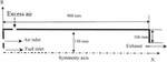
A 2D computational domain was constructed and built using Ansys design modeler. Harwell standard furnace described in [25] is a cylinder with 150 mm radius and 900 mm length connected from the left side with two tubes inside each other as the inner one is fuel inlet with 6 mm radius and the other is the air inlet with a ring shape 27.5 mm in outer radius and 16.5 mm inner radius. The excess air is injected from sides of cylinder perpendicular to jet flow with 30 mm from the jet wall with width 10 mm. The other side of the combustion cylinder is the exhaust as shown in Figure 1. The combustion chamber cylinder in Ansys’s geometry must be divided into parts to be easier to have structured mesh in Ansys meshing.

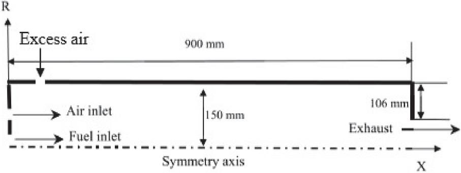
Figure 1 2D computational domain of combustor.

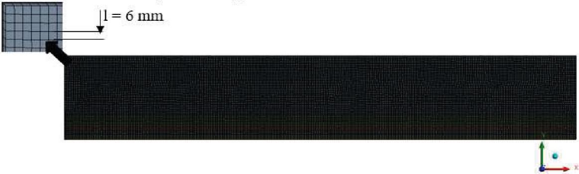
Figure 2 Meshed geometry.

2.2 Computational Grid Details and Test

Meshing is not a supplementary program, but it is a very sensitive to obtain a very good numerical result. There are two types of grid (structured and unstructured mesh. Structured mesh is preferred to make numerical results faster and accurate as shown in Figure 2. The case of turbulent flow combustion is very complicated and need a highly intensive grid and better quality to obtain a stable numerical solution. The most important areas in numerical calculations nearest the wall and the start of flame, the distance from the wall is made dimensionless [28]:

$$y^{+}=\frac{y{u}_{\tau }}{v},$$

(1)

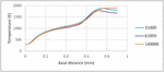
So that it should typically have a $y^{+}$ value lower than 1. If $y^{+}>1$ the mesh must be reconstructed narrower nearest the walls in the $y$ direction also the start of combustion the grid must be intensified so that this high number of grids produce the highest number of calculations. In Ansys meshing also the surfaces are defined (walls, air inlet, fuel inlet, outlet, computation domain). grid test is done 32000, 61959, 140000 cell grids at the same boundary conditions. The 140000-cell grid adds finer detail and resolves smaller scales than the courser grid thus this test showed that adding (or removing) more grid elements effects resolution but does not significantly change the general physical simulation results as shown on Figure 3 high similarity on axial temperatures on the contrary, the time required to calculate the same simulations with high number of grids will be doubled so that 61959 will be selected.

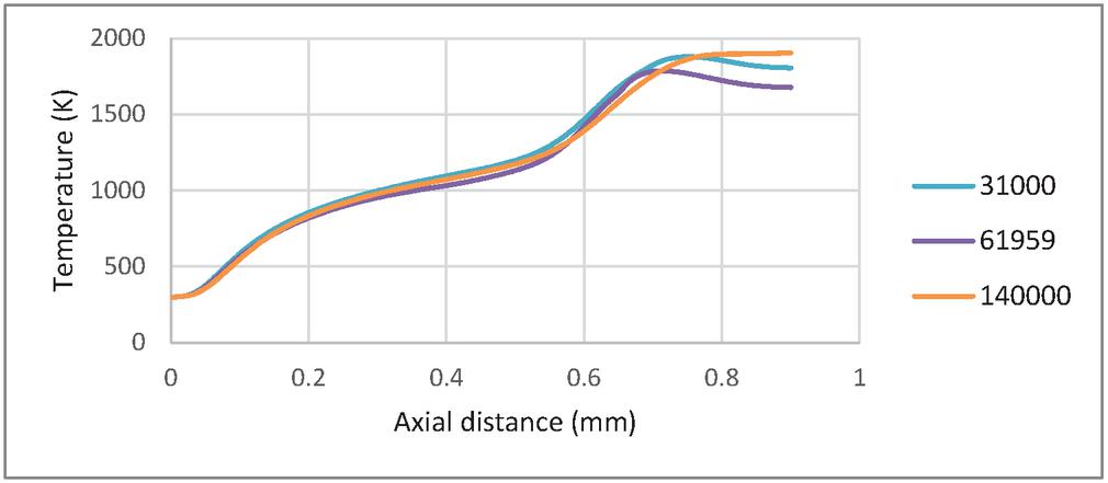
Figure 3 Temperature at centre line at grid independency test.

Ansys meshing details was applied as following use advanced size function On curvature, Relevance centre fine, Smoothing high, Min size 0.1332 mm, Max Face size 1.5 mm, Max size 3 mm, Growth rate 1.2, Minimum edge length 6 mm, Nodes 62661, Elements 61959, Average Aspect Ratio 1.31, Average skewness 1.93 e-002, Orthogonal quality 0.9967 as shown in Figure 2.

2.3 Governing Equations

The main governing equations is used in solving the problem [28].

The equation for conservation of mass, or continuity equation, can be written as follows:

$$\frac{\partial \rho }{\rho t}=\nabla \cdot (\rho \overrightarrow{v})$$

(2)

Conservation of momentum in an inertial (non-accelerating) reference frame is described by

$$\frac{\partial }{\partial t}(\rho \overrightarrow{v})+\nabla \cdot (\rho \overrightarrow{v}\overrightarrow{v})=-\nabla p+\nabla \cdot (\overline{\overline{\tau }})+\rho \overrightarrow{g}+\overrightarrow{F}$$

(3)

In the Eddy dissipation model, the reaction rate could be calculated by

$R_{i_r}$	$=MIN(R_{i_{r_{(React)}}},R_{i_{r_{(Prod)}}})$	(4)
$R_{i_{r_{(React)}}}$	$=v_{i_r}{M}_{w_i}A\rho {\displaystyle \frac{\epsilon }{K}}min\left({\displaystyle \frac{Y_i}{v_{i_r}{M}_{w_i}}}\right)$	(5)
$R_{i_{r_{(Prod)}}}$	$=v_{i_r}{M}_{w_i}AB\rho {\displaystyle \frac{\epsilon }{K}}min\left({\displaystyle \frac{{\sum }_p(Y_p)}{{\sum }_j^N{v}_{i_r}{M}_{w_j}}}\right)$	(6)

A and B are constants A $=$ 4.0 and B $=$ 0.5 suggested by Magnussen [29].

For Detached Eddy Simulation spalart-Allmaras model-based DES [30], it is modeled as

${\displaystyle \frac{D\tilde{v}}{Dt}}=C_{b1}\tilde{v}\tilde{S}-C_{w1}{f}_w{\left({\displaystyle \frac{\tilde{v}}{\overline{d}}}\right)}^2+{\displaystyle \frac{1}{{\sigma }_{\tilde{v}}}}\left[{\displaystyle \frac{\partial }{\partial x_j}}\left\{(\mu +\rho \tilde{v}){\displaystyle \frac{\partial \tilde{v}}{\partial x_j}}\right\}+\mathrm{\cdots }\right]$

(7)

2.4 Numerical Details

Using finite volume solver Ansys fluent a lot of steps must be presented; it can be explained briefly as follows:

• General setup energizes pressure-based solver because density-based is normally only used for higher Mach numbers and un-steady state simulation.

• DES is used which combining the benefits of Realizable k-epsilon and LES while minimizing their disadvantages

• Activate energy equation

• Eddy dissipation model with methane-air mixture fraction [29]. The first assumption suggested by Magnussen is being one-step chemistry and irreversible. Along with high computing speed, the EDM model is straightforward and provides convergence and reasonable accuracy [31].

Solution method for pressure velocity coupling, spatial Discretization and transient formulation is selected as following Pressure velocity coupling Scheme PISO which provides faster convergence for unsteady flows than the standard SIMPLE approach [28], Skewness correction $=$ 1, Neighbor correction $=$ 1, Spatial Discretization (Gradient $=$ Least Squares cell Based, Pressure $=$ PRESTO, Momentum $=$ Bounded central Differencing, Sub grid kinetic energy $=$ Second order upwind, Pollutant no $=$ Second order upwind, Energy $=$ Second order upwind, Mean mixture fraction $=$ Second order upwind), Transient formulation $=$ Bounded second order implicit and convergence criteria is assumed when the residual values are less than ${10}^{-6}$.

Solution control, relaxation factors in default equal 1 and it could be very aggressive for the DES model so that should be less than 0.7 to stabilize the solution as following pressure $=$ 0.5, density $=$ 0.75, energy $=$ 0.75.

2.5 Boundary Conditions

Inlet air velocity is changed sinusoidal with time, so that this equation must be written in c code and then interrupted with Ansys using UDF as shown in Figure 4.

$$v=12.8+12.8\times \sin (f\times t)$$

(8)

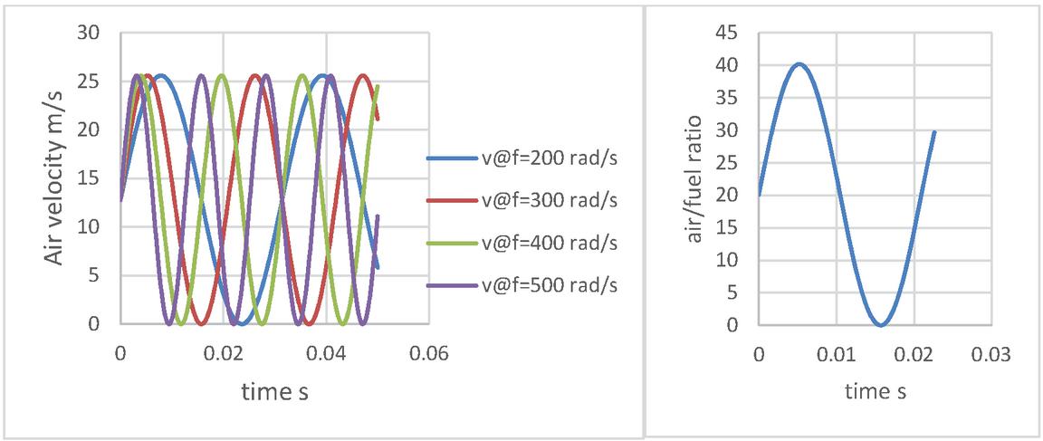
Figure 4 Inlet air velocity profile at different frequencies and its effect on air/fuel ratio.

Define the velocity equation of air as an unsteady velocity function and fuel velocity $=$ 15 m/s.

five frequencies are used with following cycle time and Strouhal number are calculated at air inlet hydraulic diameter $=$ 22 mm and air mean velocity $=$ 12.8 m/s as in Table 2.

Table 2 Cycle time and Strouhal number at different frequencies

Frequencies	f $=$ 100 rad/s	f $=$ 200 rad/s	f $=$ 300 rad/s	f $=$ 400 rad/s	f $=$ 500 rad/s
Cycle time	0.06 s	0.03 s	0.02 s	0.0157 s	0.0125s
St $=$ fD/U	0.02	0.05	0.08	0.1	0.13

Wall of combustion chamber is defined as a stationary wall with no slip. Exhaust outlet is defined as an outlet with the gauge pressure outlet=0 pascals, also adding cross excess air with velocity 10 m/s perpendicular to pulsation air inlet with frequency 500 rad/s to study improvements could be obtained.

2.6 Post Processing

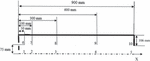
Monitors are used to save the results of T, v, NO and turbulent kinetic energy at different axial positions measured from fuel nozzle (50, 100, 300, 600, 900) mm at y $=$ 0 and 75 mm as shown in Figure 5 and to monitor residual changes with time.

Calculation activities are used to save contours of temperature with time to produce solution animation.

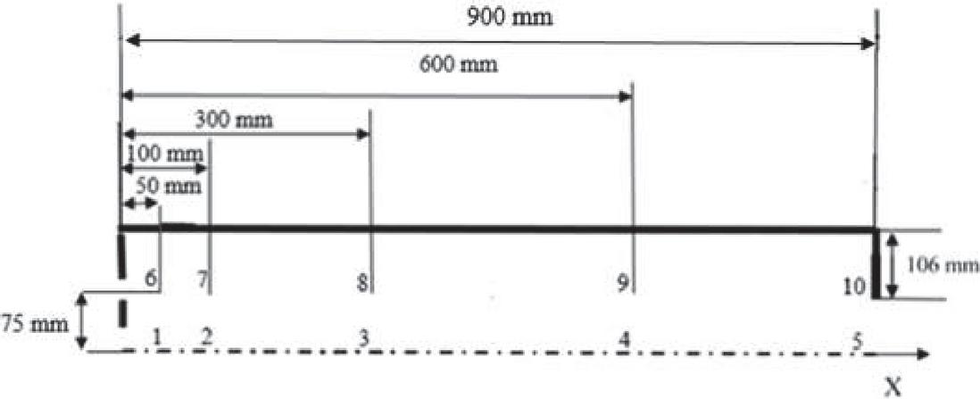
Figure 5 Calculations are done at 10 points [dimensions in mm].

2.7 Time Step Test

Run calculation is used to define time step size, time steps number and number of iterations per time step. Time step selection for large eddy simulation must be very small to provide an adequate temporal resolution of the flow as it passes through the cell so that it is selected equal 0.0005 seconds after timestep test and achieving that courant number $<$ 1 [28] to be sure that the general combustion characteristics are approximately constant as in Figure 6.

$\mathrm{\Delta }t$	$={\displaystyle \frac{\mathrm{\Delta }x}{2U}}={\displaystyle \frac{15}{2\times 12.8\times 1000}}\le 0.000585s$
$\mathrm{courant}\mathrm{number}$	$={\displaystyle \frac{\mathrm{characteristic}\mathrm{flow}\mathrm{velocity}\times \mathrm{\Delta }\mathrm{t}}{\mathrm{Tybical}\mathrm{cell}\mathrm{size}}}$
	$={\displaystyle \frac{12.8\times 0.0005}{0.015}}=0.426\le 1$

The time step test was done at three values (0.0001-0.0003-0.0005) second at the same time $=$ 3.2e-2 s which is the end of one cycle of pulsating with 500 rad/s frequency without any changes either timesteps. Obtained results show that 0.0001 s is the best as it shows more details but also 0.0005 s is acceptable also but with smaller time calculations.

Figure 6 Temperature contour of time step test (a) $\mathrm{\Delta }t=0.0001$ s, (b) $\mathrm{\Delta }t=0.0003$ s, (c) $\mathrm{\Delta }t=0.0005$ s.

Every case is applied on workstation z800 with dual processors Intel Xeon X5675, 3.1 GHz cache, and 32 GB ram for 24 hours approximately using Ain shams licenses at 61959 element and 0.0005-time step. The same case with 140000 element and 0.0001-timestep will take a week.

3 Validation of Numerical Model

Experimental study of pulsation combustion is very difficult due to high turbulent combustion and difficulty in tracking instantaneously the flame shape, temperature and variables changes. Experimental studies need high dynamic response characteristic thermocouples which can measure one thousand reading per second or high-speed camera and this is very expensive therefore computational fluid dynamics (CFD) is a good option to overcome all of these difficulties. CFD has a great difficulty because the high turbulent combustion needs extensive calculation which need large computational power, workstations having high number of cores and large number of iterations. Numerical modelling of the turbulent reacting flow in Harwell standard furnace [25] was carried out using Ansys Fluent 16. This methodology is getting increasingly popular among researchers. It was validated in a lot of researches to simulate diffusion Harwell furnace combustion. YILMAZ [25] used the same methodology to examine the effect of swirl number on combustion flow characteristics which was compared with the same experimental conditions in the study of Wilkes [26]. Figure 7 shows the great similarity between experimental [26] and numerical data. In addition, Chen [27] used the same configuration to study the effect acoustic fluctuations on combustion. So that in current study the same models are used with same furnace dimensions, time step test, grid test and converged residual values are less than ${10}^{-6}$ as shown in Figure 8 could be a very accurate investigation for pulsation combustion.

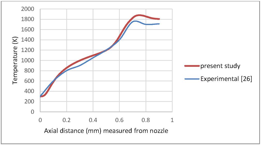
Figure 7 Validation of present study with previous work and experimental data.

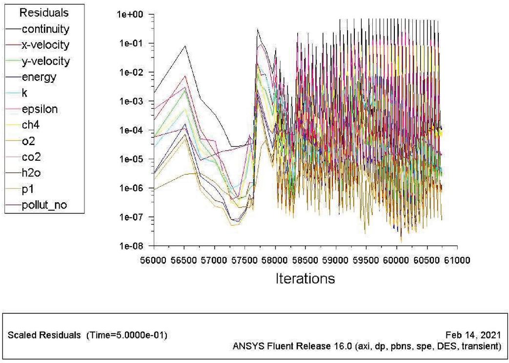
Figure 8 Variation of the residual plot.

4 Results and Discussion

4.1 Time Trace of Air Pulsation

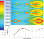
The following temperature contours shown in Figure 9 represents 12 cycles of (air-methane) mixture pulsation combustion with air frequency $=$ 500 rad/s so cycle time $=$ 0.0125 s and operation time $=$ 12 * 0.0125 $=$ 0.15 s every cycle was divided into 25-time step which help to track what happened in Harwell furnace [25]. As shown in Figure 9 that the end of first cycle (b) the changes of air velocity effect on the start of flame shape (a) by producing a small swirl in front of air jet then start the second cycle begin to push the first cycle swirls but with bigger size swirls (c). At the start of fourth cycle (d) there are a lot of swirls in sides of combustion chamber then in the start of six cycle (e) could see approximately the final shape of flame which still repeated for the end of 12 cycles (h) in this shape the flame length is decreased than the start shape (a) by 25% approximately so that pulsation of air made a great effect to increase swirls and shearing between combustion layers to produce a complete combustion in shorter distance also the area with maximum temperature decreased which decrease NO${}_{\mathrm{X}}$ formation.

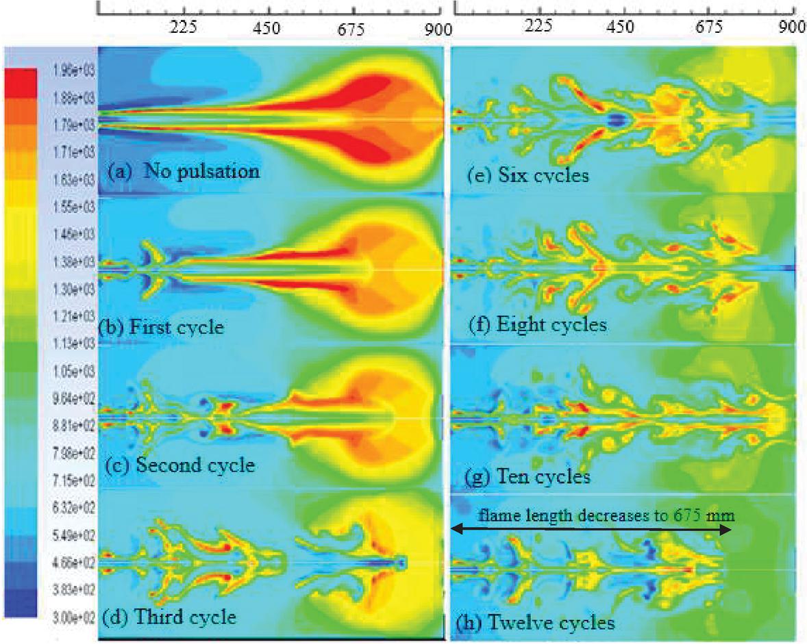
Figure 9 Temperature contour of time step test (a)$\mathrm{\Delta }t$ $=$ 0 s, (b) $\mathrm{\Delta }t$ $=$ 0.0125 s, (c) $\mathrm{\Delta }t$ $=$ 0.025 s, (d) $\mathrm{\Delta }t$ $=$ 0.0376 s (e) $\mathrm{\Delta }t$ $=$ 0.0753 s (f) $\mathrm{\Delta }t$ $=$ 0.1005s (g) $\mathrm{\Delta }t$ $=$ 0.125 s (h) $\mathrm{\Delta }t$ $=$ 0.1507 s.

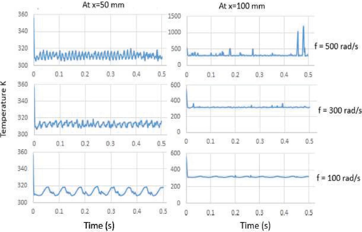
Figure 10 Effect of air frequency on temperature with time at $x=50$ mm, $x=100$ mm.

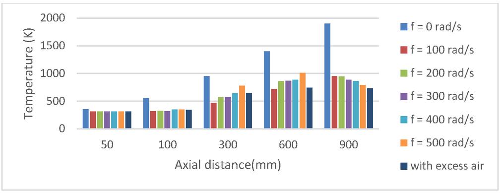
Figure 11 Effect of air frequency of average temperature at $y=0$ mm.

4.2 Effect of Frequency on Temperature

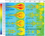
In fact, increasing air inlet frequency from 100 to 500 rad/s increase number of swirls between flow layers as shown in Figure 13. The reason for these swirls production is that when the air velocity decreased to 0 m/s the pressure in the air inlet drops which suck the fuel tangentially and when the air velocity increases again the air velocity redirect fuel axially producing a new swirl every pulse cycle time as shown in Figure 16. These swirls firstly change flow velocity direction from axial to tangential. The second role of these swirls is to increase turbulent kinetic energy and improve air-fuel mixing [25]. Tangential velocity decrease diffusion flame length and increase the average temperature near the inlet of the furnace. The flame doesn’t concentrate in the final part of combustion chamber which help to design smaller furnace dimensions. The sinusoidal air velocity magnitude change air fuel ratio from stochiometric ratio as shown in Figure 4 which in role increase cooling of the combustion furnace. This cooling decreases the time average temperature from 1900 k to 1000 k as shown in Figure 11. The temperature distribution became more uniform in all the furnace also due to shrinking of flame length make the temperature at the exhaust decreased. It could be seen at Figure 10 that increasing air frequency increase temperature frequency near the inlet which increase number of cycles during combustion time. Figure 12 shows that pulsation combustion increase radial temperature only this for $x<300$ mm but there is decrease in radial temperature at $900>x>300$ which help to distribute combustion radial and doesn’t concentrate on the middle due to shearing effect of flow. Also adding excess air perpendicular to jet nozzle increase cooling and the temperatures axial and radial decrease.

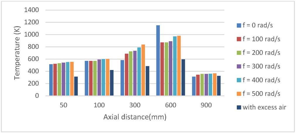
Figure 12 Effect of air frequency of average temperature at radial distance at $y=75$ mm.

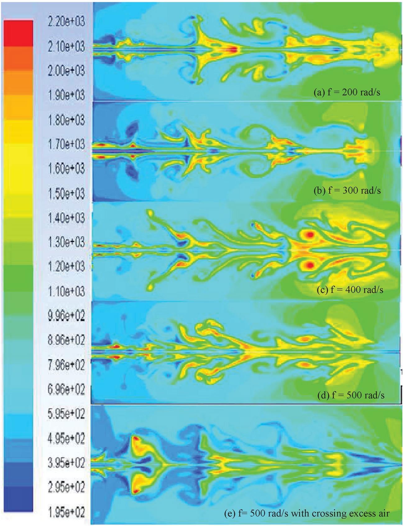
Figure 13 Temperature contour at $t$ $=$ 0.105 s for (a) $f$ $=$ 200 rad/s, (b) $f$ $=$ 300 rad/s, (c) $f$ $=$ 400 rad/s, (d)f $=$ 500 rad/s, (e) f $=$ 500 rad/s with crossing excess air.

4.3 Effect of Air Frequency on Velocity Magnitude of Combustion Products

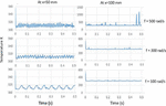
As shown on contours of temperature and Figure 16 air pulsation produce a lot of swirls produce a tangential velocity so that velocity increased in radial. Radial velocity increase shear between layers of flow and this shear produces a strongly effect on mixing between fuel and air. These fluctuations involves hot spots (entropy fluctuations) or vorticity perturbations produced by temporal variations in combustion, which generate waves as they accelerate through any restriction at the exit of the combustor. All of this made the maximum velocity values along the axis of the combustion chamber and radial increased by increasing frequency as shown in Figures 14 and 15. High velocity combustion products generated by pulse combustors can directly atomize and dry material with no need for nozzle and atomizers which require expensive pumps [32]. Adding excess air increase velocity axial but doesn’t have the same effect radial.

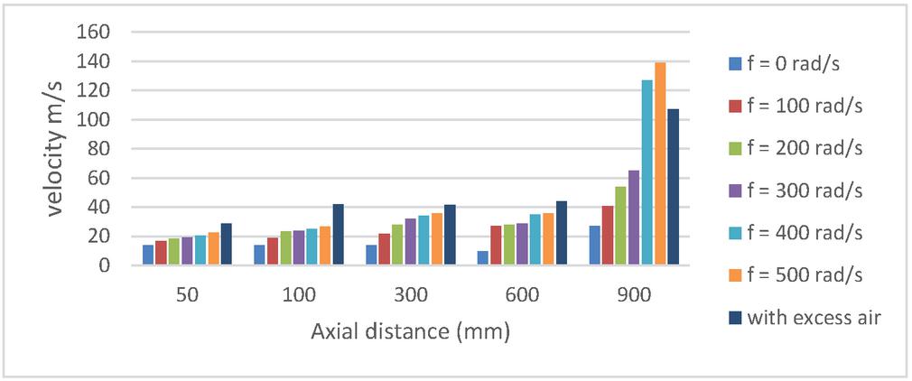
Figure 14 Air Frequency and maximum velocity during Operation at $y=0$ mm.

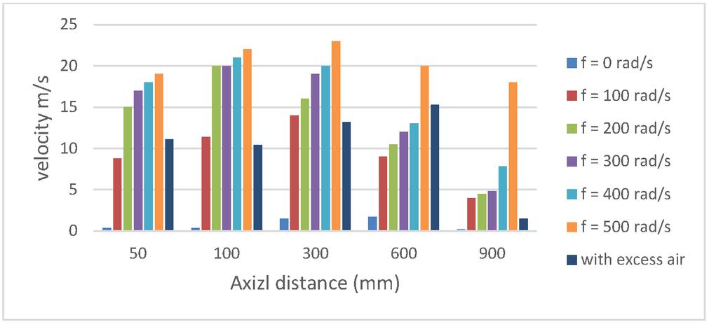
Figure 15 Air Frequency and maximum velocity during Operation radial at $y=75$ mm.

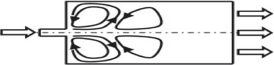
Figure 16 Velocity directions.

4.4 Effect of Air Frequency on Turbulent Kinetic Energy (TKE)

The air flow pulsation causes the flame to spread tangentially and increase shear between layers of flow which increase air fuel mixing which increase velocity as explained before which in role increase turbulent kinetic energy axial and radial by 80% as show in Figures 17 and 18 also this high turbulence leads to thickening the flame [33], reducing temperature gradients in reaction zone. Adding excess air increase turbulent kinetic energy by 10%.

Figure 17 Effect of air frequency on average TKE during Operation at $x=900$ mm, $y$ $=$ 0 mm.

Figure 18 Effect of air frequency on average TKE during operation at $x=900$ mm, $y=75$ mm.

4.5 Effect of Air Frequency on NO

NOx is a generic term for the nitrogen oxides that are most relevant to air pollution, namely nitric oxide (NO) and nitrogen dioxide (NO2). These gases contribute to the formation of smog and acid rain, as well as affecting tropospheric ozone. Figure 19 show the average mass fraction of NO along the axis of the furnace. The increasing air turbulence intensity results in decreasing NO formation [34]. NOx formation is directly related to nitrogen residence time in reaction zone, flame temperature and maximum temperature position [31]. Pulsating combustion increase turbulent kinetic energy by 80% and decrease the average temperature from 1800k to 1000k so that the amount of NO decrease by 60%. As the mass fraction of No location affected by maximum temperature position. The maximum NO produced between 600 mm and 900 mm where the maximum average temperature occurred. Pulsating combustion decreases flame length by 25% which shift the maximum combustion temperature towards the jet nozzle. The maximum mass fraction of NO at non-pulsation at 900 mm axial distance $=$ 2.5E-6. By increasing frequency, the maximum mass fraction of NO decrease and move towards the jet nozzle which is the main reason at 900 mm axial distance the pattern got reversed. The other reason for decreasing mass fraction of NO is that the flame length decreased and time of air injection decreased which decrease the reaction time between nitrogen and oxygen. Also adding excess air increase cooling which in role decrease the amount of NO.

Figure 19 Effect of air frequency of average Mass fraction of NO at axial distance.

5 Conclusion and Future Recommendations

The current research presents a numerical model of reacting flow in transient with fluctuating air inlet velocity to examine the effect of these fluctuations on combustion variables (T, v, NO, K). The obtained numerical results show that:

• Increasing flow frequency help to change both temperature and velocity direction radially and decrease flame length by 25%.

• Change the flame shape to be wider and shorter with increasing flow frequency.

• Increase mixing, uniform temperature distribution radial direction and decrease maximum temperature help to eliminate pollutant NO from 0.0001 to 0.00002.

• Increasing flow frequency increase the average kinetic energy from 0.002 to 0.05 m${}^2$/s${}^2$

• Increase maximum velocities of combustion products from 12.8 m/s to 140 m/s.

• Adding excess air increase cooling and increase velocities and decrease NO

• The findings of this research could be useful and easier application to increase furnace temperature homogeneity on surface and reduce emissions.

The most important benefit in numerical modelling is the powerful tool having a higher number of processors and more RAM (Random Access Memory) to obtain the following investigations without need of repeating experimental work.

Recommendations for future work as follows:

• Could obtain more time steps to obtain longer time of combustion.

• Could obtain the results for different combustion chamber dimensions.

• Examine the effect of pulsation combustion at different fuel types.

• Change the sinusoidal user defined function used by another type of equations.

• Change air fuel ratio by changing the velocities of air and fuel and investigate this effect with pulsation.

• Could put the air in the middle tube and the fuel in the outer one (inverse combustion).

• Try another combustion model such as non-premixed combustion model pdf.

Nomenclature

Re	$=$	Reynolds number $\equiv$ ratio of inertial forces to viscous forces
		(dimensionless)
$\nabla$	$=$	Gradient Operator
$y^{+}$	$=$	dimensionless distance from the wall
$\mu$	$=$	Dynamic viscosity (cP, Pa-s, lbm /ft-s)
$\overrightarrow{v}$	$=$	Overall velocity vector (m/s, ft/s)
f	$=$	frequency (rad/sec)
$\rho$	$=$	Density (kg/m${}^3$)
$\overrightarrow{F}$	$=$	Force vector $(N)$
H	$=$	Total enthalpy (joules/mole)
S	$=$	Total entropy (J/K)
$\overrightarrow{g}$	$=$	Gravitational acceleration (m/s2, ft/s2);
		standard values $=$ 9.80665 m/s2.
$\mathrm{\ell }$, l, L	$=$	Length scale (m, cm, ft, in)
K	$=$	Equilibrium constant
K	$=$	Turbulent kinetic energy
T	$=$	Temperature (K, o C, o R, o F)
t	$=$	Time (s)
$\sigma$	$=$	Surface tension (kg/m, dyn/cm, lbf/ft)
$C_P$	$=$	Heat capacity at constant pressure, volume (J/kg-K)
P	$=$	Pressure (Pa, atm, mm Hg)
St	$=$	Strouhal number

Subscripts

DES	$=$	Detached Eddy Simulation
TKE	$=$	Turbulent Kinetic Energy
EDM	$=$	Eddy Dissipation Model

References

[1] Shell, Royal Dutch. Shell Energy Scenarios 2050, Shell International BV. 2008.

[2] Seyboth, Kristin, et al. Recognising the potential for renewable energy heating and cooling. Energy Policy. 2008; 36.7: 2460–2463.

[3] Scotti, Alberto; Piomelli, Ugo. Turbulence models in pulsating flows. AIAA journal. 2002; 40.3: 537–544.

[4] Valaev, Alexandr Alexandrovich, Dmitry Georgievich Zhimerin, Eduard Alexandrovich Mironov, and Vladimir Andreevich Popov. “Method and apparatus for intermittent combustion.” U.S. Patent 3,954,380, issued May 4, 1976.

[5] Fureby, C., Lundgren, E. One-dimensional models for pulsating combustion. Combustion science and technology. 1993; 94.1–6: 337–351.

[6] Geng, T., Zheng, F., Kuznetsov, A. V., Roberts, W. L., and Paxson, D. E.. Comparison between numerically simulated and experimentally measured flow field quantities behind a pulsejet. Flow, turbulence and combustion. 2010; 84.4: 653–667.

[7] Akulich, P. V., Kuts, P. S., Samsonyuk, V. K., Severyanin, V. S., and Slizhuk, V. D.. Investigation of a pulsating-combustion chamber. Journal of engineering physics and thermophysics. 2000; 73.3: 477–480.

[8] Yallina, E. V., Larionov, V. M., Iovleva, O. V. Pulsating combustion of gas fuel in the combustion chamber with closed resonant circuit. In: Journal of Physics: Conference Series. IOP Publishing. 2013; p. 012017.

[9] Rafi, Shaik, Kumar, B. Kishore. Design and CFD Analysis of Pulse Jet Engine. 2016.

[10] Avinash, T., Reddy, B. Design and CFD Analysis of Pulse Jet Propulsion Engine. International Journal of Professional Engineering Studies. 2016; 7.

[11] Evans, R. G., Alshami, A. S. Pulse jet orchard heater system development: Part I. Design, construction, and optimization. Transactions of the ASABE. 2009; 52.2: 331–343.

[12] Sayres, John. Computational Fluid Dynamics for Pulsejets and Pulsejet Related Technologies. 2010.

[13] Geng, T., Kiker Jr, A., Ordon, R., Kuznetsov, A.V., Zeng, T.F. and Roberts. Combined numerical and experimental investigation of a hobby-scale pulsejet. Journal of propulsion and power. 2007; 23.1: 186–193.

[14] Schoen, Michael Alexander. Experimental investigations in 15 centimeter class pulsejet engines. 2005.

[15] Ordon, Robert Lewis. Experimental Investigations into the operational parameters of a 50 Centimeter Class Pulsejet Engine. 2006.

[16] Kiker, Adam Paul. Experimental investigations of mini-pulsejet engines. 2005.

[17] Zheng, Fei. Computational Investigation of High-Speed Pulsejets. 2009.

[18] Debnath, Pinku, Pandey, K. M. Numerical investigation of detonation combustion wave propagation in pulse detonation combustor with nozzle. Advances in aircraft and spacecraft science. 2020; 7.3: 187–202.

[19] Guan, Peng, Yanting, A. I. Study on thermal-acoustic-structural performance of Aeroengine Combustor based on Coupled-Field Technology.

[20] Yao, Wei, Ging Wang, Yang Lu. Full-scale Detached Eddy Simulation of kerosene fuelled scramjet combustor based on skeletal mechanism. In: 20th AIAA International Space Planes and Hypersonic Systems and Technologies Conference. 2015; p. 3579.

[21] Kamal, M. M. NOx emission performance of triple flames. Proceedings of the Institution of Mechanical Engineers, Part A: Journal of Power and Energy. 2007; 221.8: 1193–1208.

[22] Kamal, Mahmoud M. Development of a multiple opposing jets’ burner for premixed flames. Proceedings of the Institution of Mechanical Engineers, Part A: Journal of Power and Energy. 2012; 226.8: 1032–1049.

[23] Kamal, M. M. Development of a cylindrical burner comprising multiple pairs of opposing partially premixed or inverse diffusion flames. Proceedings of the Institution of Mechanical Engineers, Part A: Journal of Power and Energy. 2015; 229.8: 992–1006.

[24] Kamal, M. M. Combustion via multiple pairs of opposing premixed flames with a cross-flow. Proceedings of the Institution of Mechanical Engineers, Part A: Journal of Power and Energy. 2017; 231.1: 39–58.

[25] Yilmaz, Ilker. Effect of swirl number on combustion characteristics in a natural gas diffusion flame. Journal of Energy Resources Technology. 2013; 135.4.

[26] N. Wilkes, P. Guilbert, C. Shepherd, S. Simcox, UKAEA Atomic Energy Research Establishment, H. C. S., Div, S., UKAEA Atomic Energy Research Establishment. E. S. D., The Application of HARWELL-Flow3d to Combustion Problems, UKAEA Atomic Energy Research Establishment Computer Science and Systems Division, 1989.

[27] Chen, Song. Numerical study of a methane jet diffusion flame in a longitudinal tube with a standing wave. Energy Procedia, 2017; 105: 1539–1544.

[28] Fluent, A.N.S.Y.S. Theory Guide 15. Fluent Incorporated. 2013.

[29] Magnussen BF, Hjertager BH. On mathematical modelling of turbulent combustion with special emphasis on soot formation and combustion. In Symposium (international) on Combustion 1977 Jan 1 (Vol. 16, No. 1, pp. 719–729). Elsevier.

[30] Spalart PR, Shur M. On the sensitization of turbulence models to rotation and curvature. Aerospace Science and Technology. 1997 Jul 1;1(5):297–302.

[31] Hosseini AA, Ghodrat M, Moghiman M, Pourhoseini SH. Numerical study of inlet air swirl intensity effect of a Methane-Air Diffusion Flame on its combustion characteristics. Case Studies in Thermal Engineering. 2020 Apr 1;18:100610.

[32] Gray RR, Lindahl TG, Inventors; Hosokawa Micron International Inc 780 Third Avenue New York New York 10017 A Corp of, Sonodyne Industries Inc 11135 SW Capitol HWY Portland or 97219 A Corp of or, Sonodyne Industries Inc A Corp of or, Hosokawa Micron International Inc, assignee. Elevated temperature dehydration section for particle drying pulse jet combustion systems. United States patent US 4,701,126. 1987 Oct 20.

[33] Hamed AM, Moustafa AM, Kamal MM, Hussin AE. Single and Double Flow Pulsations of Normal and Inverse Partially Premixed Methane-Air Flames. Combustion Science and Technology. 2020 Dec 12:1–31.

[34] Guessab A, Aris A, Baki T, Bounif A. The Effects Turbulence Intensity on NOx Formation in Turbulent Diffusion Piloted Flame (Sandia Flame D). Recent Advances in Mechanical Engineering and Mechanics. 2011:144–50.

Biographies

Mahmoud Magdy received the bachelor’s degree in mechanical engineering from military technical college in 2012, the master’s degree in mechanical power department from Ain shams University in 2018,

European Journal of Computational Mechanics, Vol. 29_2-3, 279–302.
doi: 10.13052/ejcm2642-2085.29235
© 2021 River Publishers

Abstract

1 Introduction

2 Methodology

2.1 Computational Domain

2.2 Computational Grid Details and Test

2.3 Governing Equations

2.4 Numerical Details

2.5 Boundary Conditions

2.6 Post Processing

2.7 Time Step Test

3 Validation of Numerical Model

4 Results and Discussion

4.1 Time Trace of Air Pulsation

4.2 Effect of Frequency on Temperature

4.3 Effect of Air Frequency on Velocity Magnitude of Combustion Products

4.4 Effect of Air Frequency on Turbulent Kinetic Energy (TKE)

4.5 Effect of Air Frequency on NO

5 Conclusion and Future Recommendations

References

Biographies