A Parameter-Uniform Finite Difference Scheme for Singularly Perturbed Parabolic Problem with Two Small Parameters

Tesfaye Aga Bullo^1,*, Guy Aymard Degla² and Gemechis File Duressa¹

¹Department of Mathematics, Jimma University, Jimma, P. O. Box 378, Ethiopia

²Institut De Mathematiques et de sciences physiques, Universit D’Abomey Calavi, Benin

E-mail: tesfayeaga2@gmail.com

${}^{*}$Corresponding Author

Received 13 May 2021; Accepted 03 September 2021; Publication 06 October 2021

Abstract

A parameter-uniform finite difference scheme is constructed and analyzed for solving singularly perturbed parabolic problems with two parameters. The solution involves boundary layers at both left and right ends of the solution domain. A numerical algorithm is formulated based on uniform mesh finite difference approximation for time variable and appropriate piecewise uniform mesh for the spatial variable. Parameter-uniform error bounds are established for both theoretical and experimental results and observed that the scheme is second-order convergent. Furthermore, the present method produces a more accurate solution than some methods existing in the literature.

Keywords: Parameter-uniform, singularly perturbed, parabolic problems, two-parameters, finite difference scheme, error bounds, and accurate solution.

1 Introduction

Singular perturbation problems emerged as a result of modeling real-life applications and their solutions exhibit boundary layer phenomena. The best example to mention is the Navier-Stokes equations with large Reynolds number in fluid dynamics, the convective heat transport problems with large Péclet number, [1–3]. Based on the number of perturbation parameters, continuity or discontinuity of the coefficient; and source function or initial and/or boundary conditions throughout the considered domain, singularly perturbed parabolic problems can be categorized in various types [4–18]. From these problems singularly perturbed two-parameter parabolic problems are parabolic problems whose two highest-order derivatives are multiplied by perturbation parameters. Generally, singularly perturbed one-dimensional parabolic problems have boundary or interior or both boundary and interior layers depending on the defined data. Hence, in this work, we consider a class of singularly perturbed parabolic problems with two-parameters whose solution exhibit boundary layers. These types of problems arise in various areas of applications such as fluid dynamics (linear Navier-Stokes Equation), chemical reactor theory, heat, and mass transfer process in composite materials with small heat conduction. Classes of singularly perturbed parabolic problems involving single perturbation parameter and sub-divided into convection-diffusion and reaction-diffusion problems are recently studied [1–7].

Besides the books given by Miller et al. [8] and Roos et al. [9], few researchers tried to develop different numerical schemes to solve singularly perturbed parabolic problems with two-parameter. These literatures served us as a landmark to get a priori knowledge about the nature of the solution of these problems and helped us to get insight on how to develop the present numerical method. To mention some, spline difference scheme [10], a robust finite difference method [11], a robust layer adapted difference method [12], a parameter-uniform higher-order finite difference scheme [13–16] have been developed for solving singularly perturbed parabolic problem with two-parameters. In most of these works, fitted mesh finite difference methods have been adopted, but they gave numerical solutions with less accuracy and low rate convergence. Further, some numerical methods have been developed recently for solving different types of singularly perturbed differential-difference and differential equations aroused from modeling of real-life application [18–27].

Singular perturbed parabolic problems are recent and active research area in engineering and applied science. As a result, most numerical methods such as finite difference methods, finite element methods, and finite volume methods have been developed so far, but these methods produce satisfactory result only when the mesh length of the solution domain is less than the value of perturbation parameter [13]. Moreover, these methods are not uniformly convergent. This difficulty is occurred due to the existence of the perturbation parameter(s) that induces the boundary layer where the solutions vary rapidly and behave smoothly away from the layer.

Hence, it is necessary to develop stable, convergent, and methods that produce more accurate numerical solution for reasonable mesh length compared to perturbation parameter with higher order rate of convergence. Thus, in this work, we presented a more accurate numerical method that fulfill the criteria mentioned above for solving singularly perturbed parabolic problems with two parameters.

2 Statement of the Problem

Consider the following singularly perturbed two-parameter parabolic initial-boundary value problem on the solution domain $(x,t)\in D:=\mathrm{\Omega }\times (0,T],\mathrm{\Omega }=(0,1)$

$L_{x,t}u$

$\equiv \epsilon {\displaystyle \frac{{\partial }^{2}u}{\partial x^2}}+\mu a(x,t){\displaystyle \frac{\partial u}{\partial x}}-b(x,t)u(x,t)-{\displaystyle \frac{\partial u}{\partial t}}=f(x,t),$

subject to the initial and boundary conditions

$u(x,0)$	$=s(x),x\in \overline{\mathrm{\Omega }},u(0,t)=q_0(t),$
$u(1,t)$	$=q_1(t),t\in [0,T].$	(2)

The two perturbation parameters $\epsilon$ and $\mu$ that satisfy $0<\epsilon ,\mu \ll 1$. Coefficient functions $a(x,t),b(x,t)$ and source function $f(x,t)$ are sufficiently regular on $\overline{D}$ and content $a(x,t)\ge \alpha >0$, $b(x,t)\ge \beta >0$; $\alpha$ and $\beta$ are real numbers. Also, we assume that sufficient regularity and compatibility conditions are imposed on the functions $s(x),q_0(t),q_1(t)$, and $f(x,t)$, so that a unique solution exists. Moreover, sufficiently regularity and compatibility at the corners with the purpose of the solution and its regular component are sufficiently smooth for our analysis.

Problem given in Equations (1) and (2) exhibits two boundary layers with different width depending on the relation between the two parameters $\epsilon$ and $\mu$. For chosen $\gamma \approx {\min }_{(x,t)\in \overline{D}}\frac{b(x,t)}{a(x,t)}$ if $\alpha {\mu }^2\le \gamma \epsilon$, then the reduced problem of Equation (1) is

$$-b(x,t)u_0(x,t)-\frac{\partial u_0}{\partial t}=f(x,t),u_0(x,0)=s(x).$$

(3)

Thus, boundary layers of width $O(\sqrt{\epsilon })$ is expected in both neighborhood of $x=0$ and $x=1$ if $u_0(0,t)\ne q_0(t)$ and $u_0(1,t)\ne q_1(t)$.

If $\alpha {\mu }^2\ge \gamma \epsilon$, then reduced problem

$$\{\begin{array}{c}\mu a(x,t)\frac{\partial u_{\mu }}{\partial x}-b(x,t)u_{\mu }(x,t)-\frac{\partial u_{\mu }}{\partial t}=f(x,t),\hfill \\ u_{\mu }(x,0)=s(x)\hspace{1em}\mathrm{and}\hspace{1em}{u}_{\mu }(0,t)=q_0(t).\hfill \end{array}$$

(4)

is again singularly perturbed problem with perturbation parameter, $\mu$. This is a first-order hyperbolic equation with initial data specified along two sides $t=0$ and $x=0$ of the domain $\overline{D}$. A boundary layer of width $O(\epsilon /\mu )$ is predictable in the right neighborhood of $x=0$ if $u_{\mu }(0,t)\ne q_0(t)$, and a boundary layer of width $O(\mu )$ is expected in a left neighborhood of $x=1$ if $u_{\mu }(1,t)\ne q_1(t)$, [8, 9, 12, 15]. When the parameter $\mu =1$, the problem is the well-studied parabolic convection-diffusion problem in [1, 4] with the boundary layer of width $O(\epsilon )$ appears in the neighborhood of $x=0$ or $x=1$. While the parameter $\mu =0$, the problem is parabolic reaction-diffusion problem, [6, 16] which have two boundary layers of width $O(\sqrt{\epsilon })$ appears near $x=0$ and $x=1$. Herein this paper, we consider the problem in Equations (1) and (2), when the two perturbation parameter satisfies $0<\epsilon \ll 1$ and $0<\mu \ll 1$, for which the problem has different layer width on the opposite side of the space domain depending on the value of two perturbation parameters, $\epsilon$ and $\mu$.

3 Properties of Continuous Solution

In this section, a priori estimate for the solution $u(x,t)$ of Equations (1) and (2) on the solution domain $\overline{D}$ is established. These estimates contains continuous minimum principle bounds of the solution and its derivatives, and then parameter uniform bounds on the regular and singular components to analyze the proposed scheme. The detail proofs of both Lemma 3.1 and 3.2 below are provided in [11–17].

Lemma 3.1: (Minimum principle): Let $\phi \in C^{2,1}(\overline{D})$. If $\phi (x,t)\ge 0$, $\forall (x,t)\in \partial D$ and $L_{x,t}\phi (x,t)\le 0$, $\forall (x,t)\in D$, then $\phi (x,t)\ge 0$, $\forall (x,t)\in \overline{D}$.

A direct importance of this minimum principle is the following stability estimate

Lemma 3.2: (Uniform stability estimate). Let $u(x,t)$ be the solution of Equations (1) and (2). Then, we have

$${\parallel u\parallel }_{\overline{D}}\le C({\beta }^{-1}\parallel f(x,t)\parallel +\max (|q_0(t)|+|q_1(t)|)),\forall (x,t)\in \overline{D}.$$

where $\parallel .\parallel$ denotes the maximum norm on the domain $\overline{D}$, and $\beta$ is a positive constant specified under Section 2.

The solution $u(x,t)$and its derivatives satisfy the following bounds.

Lemma 3.3: For any non-negative integers $i,j$ such that $0\le i+3j\le 4$, the solution $u(x,t)$ satisfies

$${\parallel \frac{{\partial }^{i+j}u}{\partial x^{{}^i}\partial t^{{}^j}}\parallel }_{\overline{D}}\le C\{\begin{array}{cc}\frac{1}{{\left(\sqrt{\epsilon }\right)}^i},\hfill & \mathit{if}\alpha {\mu }^2\le \gamma \epsilon ,\hfill \\ {\left(\frac{\mu }{\epsilon }\right)}^i,\hfill & \mathit{if}\alpha {\mu }^2\ge \gamma \epsilon .\hfill \end{array}$$

where the constant C is independent of $\epsilon ,\mu$ and is dependent only on

$${\parallel \frac{{\partial }^{(p)}a}{\partial x^{{}^p}}\parallel }_{\overline{D}},{\parallel \frac{{\partial }^{(p)}b}{\partial x^{{}^p}}\parallel }_{\overline{D}}\mathit{\hspace{1em}}\text{and}\mathit{\hspace{1em}}{\parallel \frac{{\partial }^{(p)}f}{\partial x^{{}^p}}\parallel }_{\overline{D}},\text{for }p=0,1,2.$$

Proof. See [13].

Further to fix more firm error analysis for the proposed finite difference scheme; the solution $u(x,t)$ can be split as

$$u(x,t)=v(x,t)+w_L(x,t)+w_R(x,t),\forall (x,t)\in \overline{D}.$$

(5)

where, $v(x,t)$ is the smooth or regular component,$w_L(x,t)$ and $w_R(x,t)$ are the left and right singular components of the solution respectively.

Theorem 3.1: For all non-negative integers $i,j$ such that $0\le i+3j\le 4$, the regular component $v(x,t)$ satisfies the bounds

$${\parallel \frac{{\partial }^{i+j}v}{\partial x^{{}^i}\partial t^{{}^j}}\parallel }_{\overline{D}}\le C\{\begin{array}{cc}1+\frac{1}{{(\sqrt{\epsilon })}^{i-3}},\hfill & \text{for }\alpha {\mu }^2\le \gamma \epsilon ,\hfill \\ 1+{\left(\frac{\epsilon }{\mu }\right)}^{3-i},\hfill & \text{for }\alpha {\mu }^2\ge \gamma \epsilon \hfill \end{array}$$

where, constant C is independent of both the perturbation parameters $\epsilon$ and $\mu$. Detail proof of this theorem is given by Gupta et al. [13].

Lemma 3.4: When the solution to the problem in Equations (1) and (2) is decomposed as Equation (5), the layer component $w_L(x,t)$ and $w_R(x,t)$ satisfy the following bounds and its proof is given by O’Riordan et al. [14].

$$|w_L(x,t)|\le C\exp (-{\theta }_{1}x),|w_R(x,t)|\le C\exp (-{\theta }_2(1-x)),$$

where,

$${\theta }_1=\{\begin{array}{cc}\sqrt{\frac{\gamma \alpha }{\epsilon }},\hfill & \alpha {\mu }^2\le \gamma \epsilon ,\hfill \\ \frac{\alpha \mu }{\epsilon },\hfill & \alpha {\mu }^2\ge \gamma \epsilon ,\hfill \end{array}\mathit{\hspace{1em}}\mathrm{and}\mathit{\hspace{1em}}{\theta }_2=\{\begin{array}{cc}\frac{1}{2}\sqrt{\frac{\gamma \alpha }{\epsilon }},\hfill & \alpha {\mu }^2\le \gamma \epsilon ,\hfill \\ \frac{\gamma }{2\mu },\hfill & \alpha {\mu }^2\ge \gamma \epsilon .\hfill \end{array}$$

4 Description of the Scheme

To describe the scheme, the argument splits into two steps; the time variable is discretized on uniform mesh and then the discretization of space variable on the piecewise uniform mesh will obtain the required scheme as follow:

4.1 Temporal Discretization

To discretize the time variable with uniform mesh size k, the interval $[0,T]$ is partitioned into N equal sub-intervals and each nodal point satisfies $0=t_0<t_1<\mathrm{\cdots }<t_N=T$, for $t_n=nk$, $k=\frac{T}{N},$ $n=0,1,2,\mathrm{\dots },N$. Now, at the point $(x,t_{n+\frac{1}{2}})$, Equation (1) can be written as

$$\left(\epsilon \frac{{\partial }^{2}u}{\partial x^2}+\mu a\frac{\partial u}{\partial x}-bu-\frac{\partial u}{\partial t}\right)(x,t_{n+\frac{1}{2}})=f(x,t_{n+\frac{1}{2}}).$$

(6)

By Taylor’s series expansion about the point $(x,t_{n+\frac{1}{2}})$, we have

$$\{\begin{array}{ccc}\hfill u(x,t_{n+1})& \hfill =\hfill & u(x,t_{n+\frac{1}{2}})+\frac{k}{2}\frac{\partial u}{\partial t}u(x,t_{n+\frac{1}{2}})\hfill \\ & & +\frac{k^2}{8}\frac{{\partial }^{2}u}{\partial t^2}u(x,t_{n+\frac{1}{2}})+\frac{k^3}{48}\frac{{\partial }^{3}u}{\partial t^3}u(x,t_{n+\frac{1}{2}})+\mathrm{\cdots }\hfill \\ \hfill u(x,t_n)& \hfill =\hfill & u(x,t_{n+\frac{1}{2}})-\frac{k}{2}\frac{\partial u}{\partial t}u(x,t_{n+\frac{1}{2}})\hfill \\ & & +\frac{k^2}{8}\frac{{\partial }^{2}u}{\partial t^2}u(x,t_{n+\frac{1}{2}})-\frac{k^3}{48}\frac{{\partial }^{3}u}{\partial t^3}u(x,t_{n+\frac{1}{2}})+\mathrm{\cdots }\hfill \end{array}$$

which gives

$$\frac{\partial u}{\partial t}(x,t_{n+\frac{1}{2}})=\frac{u(x,t_{n+1})-u(x,t_n)}{k}+{\tau }_T,$$

(7)

where

$${\tau }_T=-\frac{k^2}{24}\frac{{\partial }^{3}u}{\partial t^3}u(x,t_{n+\frac{1}{2}})+\mathrm{\cdots }\equiv O(k^2).$$

This indicates, the local error estimate of time discretization is given by

$${\parallel T_{n+1}\parallel }_{\mathrm{\infty }}\le C_1{k}^3,$$

(8)

where $C_1=\frac{1}{48}\parallel \frac{{\partial }^{3}u}{\partial t^3}u(x,t_{n+\frac{1}{2}})\parallel$, is a positive constant independent of parameters $\epsilon ,\mu$ and k.

Lemma 4.1: (Global error estimate for temporal discretization). With the help of Equation (8), we have

$$\parallel E_n\parallel \le C{k}^2.$$

(9)

Proof: Using the local error estimate given in Equation (8), we get the following global error estimate at $(n+1)th$ time step

${\parallel E_{n+1}\parallel }_{\mathrm{\infty }}$	$={\parallel {\displaystyle \sum _{i=1}^N}{T}_i\parallel }_{\mathrm{\infty }},N\le {\displaystyle \frac{T}{k}}$
	$\le {\parallel T_1\parallel }_{\mathrm{\infty }}+{\parallel T_2\parallel }_{\mathrm{\infty }}+\mathrm{\cdots }+{\parallel T_N\parallel }_{\mathrm{\infty }}\le C_1(nk)k^2,$
	$\mathrm{\hspace{1em}\hspace{1em}}nk\le N,\mathrm{using}\mathrm{Equation}(8)$
	$\le N{C}_1{k}^2,\mathrm{But}C=N{C}_1$
	$\le C{k}^2,$

where $C$ is a constant independent of perturbation parameters and mesh size k.

From Equation (6), let take the average of all terms except the term involve time derivative written as

$\epsilon u_{xx}(x,t_{n+\frac{1}{2}})+\mu a(x,t_{n+\frac{1}{2}})u_x(x,t_{n+\frac{1}{2}})$
$\mathrm{\hspace{1em}\hspace{1em}}\mathit{\hspace{1em}}-b(x,t_{n+\frac{1}{2}})u(x,t_{n+\frac{1}{2}})-f(x,t_{n+\frac{1}{2}})$
$\mathrm{\hspace{1em}\hspace{1em}}={\displaystyle \frac{1}{2}}(L_{x,f}^{*}u(x,t_{n+1})+L_{x,f}^{*}u(x,t_n)),$	(10)

where $L_{x,f}^{*}u(x,t_n)=L_x^{*}u(x,t_n)-f(x,t_n),$

$$L_x^{*}u(x,t_n)=\epsilon u_{xx}(x,t_n)+\mu a(x,t_n)u_x(x,t_n)-b(x,t_n)u(x,t_n).$$

Substituting both Equation (7) and (10) into Equation (6) yields

$\left(L_x^{*}-{\displaystyle \frac{2}{k}}I\right)u(x,t_{n+1})$	$=f(x,t_{n+1})+f(x,t_n)$
	$\mathrm{\hspace{1em}}-\left(L_x^{*}+{\displaystyle \frac{2}{k}}I\right)u(x,t_n),$	(11)

subject to the initial and boundary conditions

$u(0,t_{n+1})$	$=q_0(t_{n+1}),u(1,t_{n+1})=q_1(t_{n+1}),$
$u(x,0)$	$=s(x),\forall x\in (0,1).$	(12)

This semi-discrete approximation $u(x,t_{n+1})$ of Equations (11) and (12) to the exact solution $u(x,t)$ of Equations (1) and (2) at the time levels $t_{n+1}=(n+1)k$.

4.2 Space Mesh Generation and Numerical Discretization

Consider the solution has large gradients in both a narrow region near $x=0$ and $x=1$, then the mesh in this region will be fine and coarse everywhere else. Let $M$ be a positive integer such that $M=2^r$ with $r\ge 3$. The piecewise uniform Shishkin mesh type on the domain ${\overline{\mathrm{\Omega }}}^M$ is defined by partitioning the domain $\overline{\mathrm{\Omega }}=[0,1]$ into three sub-intervals ${\overline{\mathrm{\Omega }}}_1=[0,{\tau }_1]$, ${\overline{\mathrm{\Omega }}}_2=[{\tau }_1,1-{\tau }_2]$ and ${\overline{\mathrm{\Omega }}}_3=[1-{\tau }_2,1]$ which are subdivided uniformly to contain $\frac{M}{4},\frac{M}{2}$ and $\frac{M}{4}$ mesh elements respectively such that $\overline{\mathrm{\Omega }}={\overline{\mathrm{\Omega }}}_1\bigcup {\overline{\mathrm{\Omega }}}_2\bigcup {\overline{\mathrm{\Omega }}}_3$. Transition parameters ${\tau }_1$ and ${\tau }_2$ are chosen to be

${\tau }_1$	$=\{\begin{array}{cc}\min \{{\displaystyle \frac{1}{4}},2\sqrt{{\displaystyle \frac{\epsilon }{\gamma \alpha }}}\ln (M)\},\hfill & \alpha {\mu }^2\le \gamma \epsilon ,\hfill \\ \min \{{\displaystyle \frac{1}{4}},2{\displaystyle \frac{\epsilon }{\alpha \mu }}\ln (M)\},\hfill & \alpha {\mu }^2\ge \gamma \epsilon ,\hfill \end{array}$
${\tau }_2$	$=\{\begin{array}{cc}\min \{{\displaystyle \frac{1}{4}},4\sqrt{{\displaystyle \frac{\epsilon }{\gamma \alpha }}}\ln (M)\},\hfill & \alpha {\mu }^2\le \gamma \epsilon ,\hfill \\ \min \{{\displaystyle \frac{1}{4}},4{\displaystyle \frac{\mu }{\gamma }}\ln (M)\},\hfill & \alpha {\mu }^2\ge \gamma \epsilon .\hfill \end{array}.$

Moreover, the set of mesh points determined by

$$x_m=m{h}_m,m=1,2,\mathrm{\dots },M-1,\mathrm{for}{x}_0=0\mathit{\hspace{1em}}\mathrm{and}\mathit{\hspace{1em}}{x}_M=1.$$

The mesh spacing $h_m=x_m-x_{m-1}$ is given by

$$h_m=\{\begin{array}{cc}\frac{4{\tau }_1}{M},\hfill & \mathrm{if}m=1,2,\mathrm{\dots },\frac{M}{4},\hfill \\ \frac{2(1-{\tau }_2-{\tau }_1)}{M},\hfill & \mathrm{if}m=\frac{M}{4}+1,\frac{M}{4}+2,\mathrm{\dots },\frac{3M}{4},\hfill \\ \frac{4{\tau }_2}{M},\hfill & \mathrm{if}m=\frac{3M}{4}+1,\mathrm{\dots },M.\hfill \end{array}$$

(13)

We represent the full discretization mesh by $D_M^N$ and for the rest of the paper, any function $F(x,t)$ adopts the notation $F(x_m,t_n)=F_m^n$. We discretize the problem in Equation (12) on $D_M^N$ as:

$L_M^N{U}_m^n$	$:\equiv L_{M,N}^{*}{U}_m^{n+1}-{\displaystyle \frac{2}{k}}{U}_m^{n+1}$
	$\mathrm{ }=f_m^{n+1}+f_m^n-L_{M,N}^{*}{U}_m^n-{\displaystyle \frac{2}{k}}{U}_m^n,$	(14)

for $m=1,2,\mathrm{\dots },M-1$ and $n=0,1,2,\mathrm{\dots },N$. subject to the boundary and initial conditions

$$U_0^{n+1}=q_0(t_{n+1}),U_M^{n+1}=q_1(t_{n+1})\mathit{\hspace{1em}}\mathrm{and}\mathit{\hspace{1em}}{U}_m^0=u_0(x_m),$$

(15)

where

$L_{M,N}^{*}{U}_m^{n+1}$	$=\epsilon {\delta }_x^2{U}_m^{n+1}+\mu a_m^{n+1}{\delta }_x^0{U}_m^{n+1}-b_m^{n+1}{U}_m^{n+1}.$
$L_{M,N}^{*}{U}_m^n$	$=\epsilon {\delta }_x^2{U}_m^n+\mu a_m^n{\delta }_x^0{U}_m^n-b_m^n{U}_m^n.$
${\delta }_x^2{U}_m^n$	$={\displaystyle \frac{2}{h_m+h_{m+1}}}\left({\delta }_x^{+}{U}_m^n-{\delta }_x^{-}{U}_m^n\right),$
${\delta }^0{U}_m^n$	$={\displaystyle \frac{U_{m+1}^n-U_{m-1}^n}{h_m+h_{m+1}}},$
${\delta }_x^{+}{U}_m^n$	$={\displaystyle \frac{U_{m+1}^n-U_m^n}{h_{m+1}}},$
${\delta }_x^{{}^{-}}{U}_m^n$	$={\displaystyle \frac{U_m^n-U_{m-1}^n}{h_m}}.$

The obtained scheme in Equation (14) can be written in the form:

$$E_m{U}_{m-1}^{n+1}-F_m{U}_m^{n+1}+G_m{U}_{m+1}^{n+1}=H_m^{n+1},$$

(16)

where

$E_m$	$={\displaystyle \frac{2\epsilon }{h_m(h_m+h_{m+1})}}-{\displaystyle \frac{\mu a_m^{n+1}}{h_m+h_{m+1}}},$
$F_m$	$={\displaystyle \frac{2\epsilon }{h_m{h}_{m+1}}}+b_m^{n+1}+{\displaystyle \frac{2}{k}},$
$G_m$	$={\displaystyle \frac{2\epsilon }{h_m(h_m+h_{m+1})}}+{\displaystyle \frac{\mu a_m^{n+1}}{h_m+h_{m+1}}},$
$H_m^{n+1}$	$=\left({\displaystyle \frac{-2\epsilon }{h_m(h_m+h_{m+1})}}+{\displaystyle \frac{\mu a_m^{n+1}}{h_m+h_{m+1}}}\right)U_{m-1}^n$
	$\mathrm{\hspace{1em}}+\left({\displaystyle \frac{2\epsilon }{h_m{h}_{m+1}}}+b_m^n-{\displaystyle \frac{2}{k}}\right)U_m^n$
	$\mathrm{\hspace{1em}}-\left({\displaystyle \frac{2\epsilon }{h_{m+1}(h_m+h_{m+1})}}+{\displaystyle \frac{\mu a_m^{n+1}}{h_m+h_{m+1}}}\right)U_{m+1}^n+f_m^{n+1}+f_m^n$

5 Stability and Convergence Analysis

In this section, we study the stability and consistency estimate for the presented finite difference scheme of Equations (14) and (15) and establish the parameter uniform error estimate.

Lemma 5.1: Let $M_0$ be the smallest positive integer such that

$$\max \{\frac{{\parallel a\parallel }_{\overline{D}}}{\alpha },\frac{{\parallel b\parallel }_{\overline{D}}+k^{-1}}{\alpha \gamma }\}<\frac{M_0}{\ln M_0},$$

(17)

then for any $M\ge M_0$ the discretization in Equation (14) satisfies a discrete minimum principle stated as, for any mesh function ${\varphi }_m^n$ defined on ${\overline{D}}_M^N$ such that if $\varphi (x_m,t_n)$, $\forall (x_m,t_n)\in \partial D_M^N$ and $L_M^N\varphi (x_m,t_n)=L_M^N{\varphi }_m^n\le 0$, $\forall (x_m,t_n)\in \partial D_M^N$, then $\varphi (x_m,t_n)={\varphi }_m^n\ge 0$, $\forall (x_m,t_n)\in {\overline{D}}_M^N$.

Proof. Under the assumption of Equation (17), entries of the matrix related to the operator $L_M^N$ satisfies the criteria for M-matrix and associated matrix is the negative of an M-matrix.

Let $(s,y)$ be such that ${\varphi }_s^y={\min }_{(m,n)\in \overline{D}}{\varphi }_m^n<0$. Hence, $(x_s,t_y)\notin \partial D$ or $(x_s,t_y)\in D$, it follows from the definition of the point $(x_s,t_y)$, ${\varphi }_{ss}(x_s,t_y)\ge 0$, ${\varphi }_s(x_s,t_y)=0={\varphi }_y(x_s,t_y)$. Thus, $L_M^N{\varphi }_s^y>0$, which is a contradiction. Therefore, ${\varphi }_s^y\ge 0$ which implies ${\varphi }_m^n\ge 0$, $\forall (x_m,t_n)\in {\overline{D}}_M^N$.

Discrete minimum principle ensures the uniform stability of the difference operator $L_M^N$ in maximum norm.

Lemma 5.2: (Uniform stability estimate) Let $U_m^{n+1}$ be a mesh function at $(n+1)th$ a time level such that $U_0^{n+1}=U_M^{n+1}=0$. Then

$|U_m^{n+1}|$	$\le {\displaystyle \frac{1}{b_0}}\underset{1\le i\le M-1}{\max }|L_M^N{U}_i^{n+1}|,\mathrm{for}\mathit{\hspace{1em}}1\le m\le M-1,$
	$\mathrm{\hspace{1em}\hspace{1em}}\mathit{\hspace{1em}}\mathrm{and}\mathit{\hspace{1em}}0\le n\le N.$

Proof. Consider the mesh function

${({\xi }^{\pm })}_m^{n+1}$	$={\displaystyle \frac{1}{b_0}}\underset{1\le i\le M-1}{\max }|L_M^N{U}_i^{n+1}|\pm U_m^{n+1},1\le m\le M-1,$
	$\mathrm{\hspace{1em}\hspace{1em}}\mathit{\hspace{1em}}\mathrm{and}\mathit{\hspace{1em}}0\le n\le N,$

with $b_m^{n+1}\ge b_0>0$ to guarantee the uniqueness of the solution to Equation (14).

Also assume that ${({\xi }^{\pm })}_0^{n+1}\ge 0$ and ${({\xi }^{\pm })}_M^{n+1}\ge 0$, for $0\le n\le N$, then

$$L_M^N{({\xi }^{\pm })}_m^{n+1}=\frac{-b_m^{n+1}}{b_0}\underset{1\le i\le M-1}{\max }|L_M^N{U}_i^{n+1}|\pm L_M^N{U}_m^{n+1},$$

$$1\le m\le M-1,\mathrm{and}\mathit{\hspace{1em}}0\le n\le N$$

On behalf of $0\le m\le M-1$, $\frac{-b_m^{n+1}}{b_0}\le -1$. This leads to $L_M^N{({\xi }^{\pm })}_m^{n+1}\le 0$.

By the discrete minimum principle (Lemma 5.1), we conclude that $L_M^N{({\xi }^{\pm })}_m^{n+1}\ge 0$, and ${({\xi }^{\pm })}_m^{n+1}\ge 0$, $\forall 0\le m\le M$, $0\le n\le N$, and this finishes the proof.

The consistency result estimation of the truncation error bound for different operator given in Equation (14) and the convergence of the scheme will be analyzed on piecewise uniform meshes of the space variable and then using the error estimated for time discretization in Equation (9), we will conclude its order of convergence. Let $u$ be the solution to the continuous problem of Equations (1) and (2), and U be the solution to the corresponding discrete problem of Equations (14) and (15). Then at each point, the local truncation error $T_m^n$ corresponding to the operator L for an arbitrary spatial mesh with mesh size $h_m$ is given by

$T_m^n$	$=L_M^N(u-U)$
	$=\epsilon {\displaystyle \frac{d^2{u}_m^{n+1}}{d{x}^2}}+\mu a_m^{n+1}{\displaystyle \frac{d{u}_m^{n+1}}{dx}}-\epsilon {\delta }_x^2{U}_m^{n+1}-\mu a_m^{n+1}{\delta }_x^0{U}_m^{n+1}.$	(18)

Taking Taylor series expansion to $U_m^{n+1}$ around $x_m$, we get the approximations for $U_{m-1}^{n+1}$ and $U_{m+1}^{n+1}$ as

$U_{m+1}^{n+1}$	$=U_m^{n+1}+h_{m+1}{(U_m^{n+1})}^{\prime }+{\displaystyle \frac{1}{2}}{h}_{m+1}^2{(U_m^{n+1})}^{\prime \prime }+{\displaystyle \frac{1}{6}}{h}_{m+1}^3{(U_m^{n+1})}^{\prime \prime \prime }$
	$\mathrm{\hspace{1em}}+O(h_{m+1}^4).$
$U_{m-1}^{n+1}$	$=U_m^{n+1}-h_m{(U_m^{n+1})}^{\prime }+{\displaystyle \frac{1}{2}}{h}_m^2{(U_m^{n+1})}^{\prime \prime }-{\displaystyle \frac{1}{6}}{h}_m^3{(U_m^{n+1})}^{\prime \prime \prime }+O(h_m^4).$

From these two equations, we obtain

${\displaystyle \frac{U_{m+1}^{n+1}-U_m^{n+1}}{h_{m+1}}}$	$={(U_m^{n+1})}^{\prime }+{\displaystyle \frac{1}{2}}{h}_{m+1}{(U_m^{n+1})}^{\prime \prime }+{\displaystyle \frac{1}{6}}{h}_{m+1}^2{(U_m^{n+1})}^{\prime \prime \prime }$
	$\mathrm{\hspace{1em}}+O(h_{m+1}^3).$	(19)
${\displaystyle \frac{U_m^{n+1}-U_{m-1}^{n+1}}{h_m}}$	$={(U_m^{n+1})}^{\prime }-{\displaystyle \frac{1}{2}}{h}_m{(U_m^{n+1})}^{\prime \prime }+{\displaystyle \frac{1}{6}}{h}_m^2{(U_m^{n+1})}^{\prime \prime \prime }+O(h_m^3).$	(20)
${\displaystyle \frac{U_{m+1}^{n+1}-U_{m-1}^{n+1}}{h_m+h_{m+1}}}$	$={(U_m^{n+1})}^{\prime }+{\displaystyle \frac{h_{m+1}-h_m}{2}}{(U_m^{n+1})}^{\prime \prime }$
	$\mathrm{\hspace{1em}}+{\displaystyle \frac{h_m^3+h_{m+1}^3}{6(h_m+h_{m+1})}}{(U_m^{n+1})}^{\prime \prime \prime }+\mathrm{\cdots }.$	(21)

Substituting Equations (19)–(21) into Equation (18) and after small algebraic manipulation yields

$T_m^n$	$=-(h_{m+1}-h_m){\displaystyle \frac{\mu a_m^{n+1}}{2}}{(U_m^{n+1})}^{\prime \prime }$
	$\mathrm{\hspace{1em}}-\left({\displaystyle \frac{\epsilon }{3}}(h_{m+1}-h_m)+{\displaystyle \frac{\mu a_m^{n+1}(h_m^3+h_{m+1}^3)}{6(h_m+h_{m+1})}}\right){(U_m^{n+1})}^{\prime \prime \prime }+\mathrm{\cdots }$	(22)

The solution $U_m^{n+1}$ of the discrete problem in Equations (14) and (15) is decomposed into regular part V and singular part W analogously to the decomposition of continuous solution in Equation (5) as:

$$U_m^{n+1}=V_m^{n+1}+{\left(W_L\right)}_m^{n+1}+{\left(W_R\right)}_m^{n+1}.$$

where V is the solution of the nonhomogeneous problem

$$L_M^N{V}_m^{n+1}=f_m^{n+1},\forall (x_m,t_{n+1})\in D_M^N,$$
$$V_m^{n+1}=v_m^{n+1},\forall (x_m,t_{n+1})\in \partial D_M^N.$$	(23)

where W is the solution of the homogeneous problem given by

$L_M^N{(W_L)}_m^{n+1}$	$=0,\forall (x_m,t_{n+1})\in D_M^N,$
${(W_L)}_m^{n+1}$	$={(w_L)}_m^{n+1},\forall (x_m,t_{n+1})\in \partial D_M^N.$	(24)
$L_M^N{(W_R)}_m^{n+1}$	$=0,\forall (x_m,t_{n+1})\in D_M^N,$
${(W_R)}_m^{n+1}$	$={(w_R)}_m^{n+1},\forall (x_m,t_{n+1})\in \partial D_M^N.$	(25)

Therefore, the error in discrete solution can be decomposed into

$${(u-U)}_m^{n+1}={(v-V)}_m^{n+1}+{(w_L-W_L)}_m^{n+1}+{(w_R-W_R)}_m^{n+1},$$

$$\forall (x_m,t_{n+1})\in {\overline{D}}_M^N.$$

Following the procedures given in [13, 14], to establish the parameter – uniform error estimate for singular component, we define the following barrier functions

${\psi }_m^L$	$=\{\begin{array}{cc}{\displaystyle \prod _{i=1}^m}{(1+{\theta }_1{h}_m)}^{-1},\hfill & 1\le m\le M,\hfill \\ 1,\hfill & m=0\hfill \end{array}$
${\psi }_m^R$	$=\{\begin{array}{cc}{\displaystyle \prod _{i=m+1}^m}{(1+{\theta }_2{h}_m)}^{-1},\hfill & 0\le m\le M-1,\hfill \\ 1,\hfill & m=M.\hfill \end{array}$	(26)

which satisfies the inequality

$$L_M^N{\psi }_m^L\le 0\mathit{\hspace{1em}}\mathrm{and}\mathit{\hspace{1em}}{L}_M^N{\psi }_m^R\le 0,\forall 0\le m\le M.$$

(27)

Lemma 5.3: The layer components $W_L(x_m,t_n)$ and $W_R(x_m,t_n)$ satisfy the bounds

$|W_L(x_m,t_n)|$	$\le |W_L(x_0,t_n)|{\psi }_m^L,$
$|W_R(x_m,t_n)|$	$\le |W_R(x_M,t_n)|{\psi }_m^R,\forall (x_m,t_n)\in {\overline{D}}_M^N.$

Moreover, layer components $W_L(x_m,t_n)$ and $W_R(x_m,t_n)$ satisfy the following estimates in their respective no layer regions

$|W_L(x_m,t_n)|\le C{M}^{-2},\forall M/4\le m\le M,nk\le T,$

$|W_R(x_m,t_n)|\le C{M}^{-2},\forall \mathrm{\hspace{0.25em}0}\le m\le 3M/4,nk\le T.$

Proof. For layer component $W_L(x_m,t_n)$, we construct the barrier functions

$${\mathrm{\Phi }}_L^{\pm }(x_m,t_n)=|W_L(x_0,t_n)|{\psi }_m^L\pm W_L(x_m,t_n).$$

Consider that ${\mathrm{\Phi }}_L^{\pm }(x_m,t_n)\ge 0$, $\forall (x_m,t_n)\in \partial D_M^N$ and using Equation (27), we have

$$L_M^N{\mathrm{\Phi }}_L^{\pm }(x_m,t_n)\le 0,\forall (x_m,t_n)\in D_M^N.$$

Using the discrete minimum principle in Lemma 5.1, we obtain the essential result.

Besides, for $m\ge \frac{M}{4}$ we have

$${\psi }_m^L\le {\psi }_{\frac{M}{4}}^L={\left(1+{\theta }_1\frac{4{\tau }_1}{M}\right)}^{\frac{-M}{4}},$$

where ${\theta }_1$ and ${\tau }_1$ depends on the ratio of parameters ${\mu }^2$ to $\epsilon$ are given in the previous section respectively. Using both these choices of ${\theta }_1$ and ${\tau }_1$, we can show that

${\left(1+{\theta }_1{\displaystyle \frac{4{\tau }_1}{M}}\right)}^{\frac{-M}{4}}$	$={({(1+8M^{-1}\ln (M))}^{\frac{-M}{8}})}^2$
	$\le {(C{M}^{-1})}^2=C{M}^{-2}.$

Therefore, for $m\ge \frac{M}{4}$, we have $|W_L(x_m,t_n)|\le C{M}^{-2}$.

Similarly, we get the required bounds for the right layer component $W_R(x_m,t_n)$.

Lemma 5.4: (Error in the Left Singular Region) For $N\ge N_0$ assume Equation (17). Then left layer error component at each mesh point $(x_m,t_n)\in {\overline{D}}_M^N$ satisfies the following error estimate

$$|(w_L-W_L)(x_m,t_n)|\le \{\begin{array}{cc}C(M^{-2}{(\ln M)}^2),\hfill & \mathit{for}\alpha {\mu }^2\le \gamma \epsilon \hfill \\ C(M^{-2}{(\ln M)}^3),\hfill & \mathit{for}\alpha {\mu }^2\le \gamma \epsilon .\hfill \end{array}$$

Proof. The argument depends on the value of ${\tau }_1$. Assume that the transition parameter ${\tau }_1=\frac{1}{4}$, the mesh is uniform or $h_m=h_{m+1}=h$. If $\alpha {\mu }^2\le \gamma \epsilon$, then using Equation (22), $\frac{1}{\sqrt{\epsilon }}\le C\ln M$ and $\parallel \frac{{\partial }^j{w}_L}{\partial x^j}\parallel \le C$, ${\epsilon }^{-j/2}$ from Lemma 3.3 and 3.4, we obtain

$|L_M^N(w_L-W_L)(x_m,t_n)|$

$\mathrm{\hspace{1em}\hspace{1em}}\le C(M^{-2}\mu |{(W_m^{n+1})}_L^{\prime \prime \prime }|)\le C(M^{-2}\mu C{\epsilon }^{\frac{-3}{2}})$

$\mathrm{\hspace{1em}\hspace{1em}}\le C(k^2+M^{-2}{\displaystyle \frac{\mu }{\epsilon }}C\ln M),\le C(M^{-2}\ln M),$

$\mathrm{\hspace{1em}\hspace{1em}}\mathit{\hspace{1em}}\mathrm{Since},{\displaystyle \frac{\mu }{\epsilon }}\le {\displaystyle \frac{{\mu }^2}{\epsilon }}\le {\displaystyle \frac{\gamma }{\alpha }}=C.$

Hence, $|L_M^N(w_L-W_L)(x_m,t_n)|\le C(M^{-2}\ln M)$.

If $\alpha {\mu }^2\ge \gamma \epsilon$, then using Equation (23), $\frac{\mu }{\epsilon }\le C\ln M$ and $\parallel \frac{{\partial }^j{w}_L}{\partial x^j}\parallel \le C{(\frac{\mu }{\epsilon })}^j$ (Lemma 3.3 and 3.4), we obtain

$|L_M^N(w_L-W_L)(x_m,t_n)|$	$\le C(M^{-2}\mu |{(W_m^{n+1})}_L^{\prime \prime \prime }|)$
	$\le C\left(M^{-2}\mu C{\left({\displaystyle \frac{\mu }{\epsilon }}\right)}^3\right)$
	$\le C(M^{-2}\mu C{(\ln M)}^3),$
	$\le C(M^{-2}{(\ln M)}^3).$

Thus, $|L_M^N(w_L-W_L)(x_m,t_n)|\le C(M^{-2}{(\ln M)}^3)$.

Note that, in this case, the arbitrary constant C is independent of $\epsilon$ and h.

For the case, ${\tau }_1<\frac{1}{4}$ the mesh is a piecewise uniform. First, let us analyze the error in the outside from the left layer region, and then we proceed to analyze it in the left layer region. In the outer region, both $w_L$ and $W_L$ are small. As a result applying triangle inequality, and using Lemma 3.4, Lemma 5.3, we have

$|(w_L-W_L)(x_m,t_n)|$	$\le |w_L(x_m,t_n)|+|W_L(x_m,t_n)|,$
	$\le C(M^{-2}+\exp (-{\theta }_1{x}_m))$
	$\le C(M^{-2}+\exp (-{\theta }_1{\tau }_1)).$

Using the fact ${\theta }_1{\tau }_1=2\ln (M)$, we conclude that

$|(w_L-W_L)(x_m,t_n)|$	$\le C(M^{-2}+\exp (-2\ln (M)))$
	$=C(M^{-2}+M^{-2})=C{M}^{-2}.$

In the layer region, the truncation error estimate is given in Equation (23) leads to

$$|L_M^N(w_L-W_L)(x_m,t_n)|\le C(M^{-2}\mu |{(W_m^{n+1})}_L^{\prime \prime \prime }|.$$

If $\alpha {\mu }^2\le \gamma \epsilon$, then from $\parallel \frac{{\partial }^j{w}_L}{\partial x^j}\parallel \le C{\epsilon }^{\frac{-j}{2}}$, $\frac{1}{\sqrt{\epsilon }}\le C\ln M$ and using Lemma 5.2, we obtain

$$|L_M^N(w_L-W_L)(x_m,t_n)|\le C(M^{-2}\ln M).$$

In a similar manner for the case, $\alpha {\mu }^2\ge \gamma \epsilon$ use $\frac{\mu }{\epsilon }\le C\ln M$ and $\parallel \frac{{\partial }^j{w}_L}{\partial x^j}\parallel \le C{(\frac{\mu }{\epsilon })}^j$ one can get the required result.

Lemma 5.5: (Error in the Regular component) Assume that $N\ge N_0$ satisfies the assumption in Equation (17). Then the error in the regular component $V(x_m,t_n)$ satisfies the error estimate

$$|(v-V)(x_m,t_n)|\le C(M^{-2}).$$

Lemma 5.6: (Error in the Right Singular Component) With $N\ge N_0$ an assumption given in Equation (17), the right singular component $W_R(x_m,t_n)$ satisfies the error estimate

$$|(w_R-W_R)(x_m,t_n)|\le C(M^{-2}{(\ln M)}^2),\forall (x_m,t_n)\in {\overline{D}}_M^N$$

Proof: For the detail proves of both Lemmas 5.5 and 5.6, any interested reader can follow using the procedures in [13, 14].

Theorem 5.1: Assume that $N\ge N_0$ satisfies the assumption in Equation (17). Let $u(x,t)$ be the continuous solution of the problem Equations (1) and (2), and also $U(x_m,t_n)$ be the solution of the corresponding discrete problem of Equations (14) and (15), then at each mesh point $(x_m,t_n)\in {\overline{D}}_M^N$, the maximum pointwise error satisfies the parameter-uniform error bounds

$$|(u-U)(x_m,t_n)|\le \{\begin{array}{cc}C(M^{-2}{(\ln M)}^2+k^2),\hfill & \mathit{for}\alpha {\mu }^2\le \gamma \epsilon ,\hfill \\ C(M^{-2}{(\ln M)}^3+k^2),\hfill & \mathit{for}\alpha {\mu }^2\le \gamma \epsilon .\hfill \end{array}$$

where C is a positive constant independent of perturbation and mesh parameters.

Proof. Combining the estimates in Equation (9), Lemmas 5.4, 5.5 and 5.6 gives the required result.

6 Numerical Illustrations

In this section, two test examples are considered and numerical results are computed to demonstrate the effectiveness of the present scheme. Since the exact solution for such type of problems is not available, the maximum absolute errors at all the mesh points are evaluated using the formula

$$E_{\epsilon ,\mu }^{M,N}=\underset{0\le m\le M;\mathrm{\hspace{0.17em}0}\le n\le N}{\max }|U_m^n-U_{2m}^{2n}|.$$

where $U_m^n$ is an approximate solution obtained using a constant space mash size $h_m$ and time step k and $U_{2m}^{2n}$ is also an approximate solution produced using space step $\frac{h_m}{2}$ with time step, $\frac{k}{2}$. Likewise, we compute the numerical rates of convergence by $R=\frac{\log E_{\epsilon ,\mu }^{M,N}-\log E_{\epsilon ,\mu }^{2M,2N}}{\log 2}$.

Example 1: Consider the parabolic initial-boundary value problem

$$\epsilon \frac{{\partial }^{2}u}{\partial x^2}+\mu (1+x)\frac{\partial u}{\partial x}-u(x,t)-\frac{\partial u}{\partial t}=16x^2{\left(1-x\right)}^2,(x,t)\in (0,1)\times (0,T],$$

subject to the conditions

$$u(x,0)=0,x\in [0,1]\mathrm{and}u(0,t)=0=u(1,t),t\in [0,T].$$

Example 2: This example corresponds to the following initial boundary value problem

$$\epsilon \frac{{\partial }^{2}u}{\partial x^2}+\mu (1+x(1-x)+t^2)\frac{\partial u}{\partial x}-(1+5xt)u(x,t)-\frac{\partial u}{\partial t}=x(1-x)(e^t-1),$$

subject to the conditions: $u(x,0)=0,x\in [0,1]$ and $u(0,t)=0=u(1,t)$, $t\in [0,1]$.

Computed maximum absolute errors, rate of convergence and graphical results are provided in tabular form and in Figures as follow:

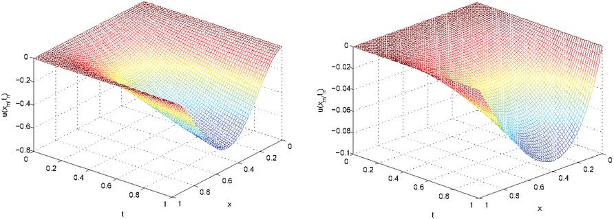
Figure 1 Solution profile for Examples 1 and 2 respectively, when $M=N=64$, $\epsilon ={10}^{-2}$ and $\mu =0.5\epsilon$.

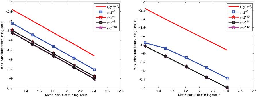
Figure 2 Log-log plot of maximum absolute errors correspond to the values of $\epsilon =2^{-5}$ for Example 1 and $\epsilon =2^{-10}$ Example 2, when $M=2N,$ $N=\{16,32,64,128,256\}$.

Table 1 Comparison of maximum absolute errors for Example 1 at $M=64$ and $k=\frac{0.125}{4}$

$\mu \downarrow$	$\epsilon ={10}^{-2}$	$\epsilon ={10}^{-4}$	$\epsilon ={10}^{-6}$	$\epsilon ={10}^{-8}$	$\epsilon ={10}^{-10}$	$\epsilon ={10}^{-12}$
Present method
${10}^{-2}$	1.5728e-05	4.2691e-03	3.6774e-05	1.2473e-05	1.2477e-05	1.2477e-05
${10}^{-4}$	1.5531e-05	6.1635e-03	1.0582e-03	1.5111e-04	1.5903e-04	1.5912e-04
${10}^{-6}$	1.5529e-05	6.1633e-03	1.0582e-03	1.0086e-04	8.5427e-06	6.7906e-06
${10}^{-8}$	1.5529e-05	6.1633e-03	1.0582e-03	1.0086e-04	8.5430e-06	6.7341e-06
${10}^{-10}$	1.5529e-05	6.1633e-03	1.0582e-03	1.0086e-04	8.5430e-06	6.7341e-06
Results in [13]
${10}^{-2}$	5.7836e-03	5.8089e-03	1.5931e-02	9.1885e-03	9.1894e-03	9.1894e-03
${10}^{-4}$	1.1314e-02	1.1271e-02	1.1273e-02	1.1290e-02	1.1291e-02	1.1291e-02
${10}^{-6}$	1.1313e-02	1.1270e-02	1.1272e-02	1.1264e-02	1.1264e-02	1.1264e-02
${10}^{-8}$	1.1313e-02	1.1270e-02	1.1272e-02	1.1264e-02	1.1263e-02	1.1263e-02
${10}^{-10}$	1.1313e-02	1.1270e-02	1.1272e-02	1.1264e-02	1.1263e-02	1.1263e-02

Table 2 Comparison of maximum absolute errors at $\epsilon =2^{-5}$, $M=2N$ and $T=1$ for Example 1

$\mu \downarrow N\to$	16	32	64	128	256
Present method
$2^{-2}$	7.4036e-04	1.8444e-04	4.6115e-05	1.1526e-05	2.8814e-06
$2^{-4}$	3.1887e-04	7.9649e-05	1.9918e-05	4.9791e-06	1.2448e-06
$2^{-6}$	2.4622e-04	6.1550e-05	1.5392e-05	3.8477e-06	9.6196e-07
$2^{-8}$	2.3900e-04	5.9701e-05	1.4927e-05	3.7318e-06	9.3297e-07
$2^{-10}$	2.3799e-04	5.9449e-05	1.4859e-05	3.7146e-06	9.2865e-07
$\mathrm{⋮}$	$\mathrm{⋮}$	$\mathrm{⋮}$	$\mathrm{⋮}$	$\mathrm{⋮}$	$\mathrm{⋮}$
$2^{-40}$	2.3770e-04	5.9375e-05	1.4841e-05	3.7100e-06	9.2748e-07
Results in [11]
$2^{-2}$	8.63e-3	3.95e-3	1.88e-3	9.20e-4	4.54e-4
$2^{-4}$	7.52e-3	3.29e-3	1.53e-3	7.35e-4	3.61e-4
$2^{-6}$	7.44e-3	3.23e-3	1.49e-3	7.18e-4	3.51e-4
$2^{-8}$	7.43e-3	3.23e-3	1.49e-3	7.16e-4	3.51e-4
$2^{-10}$	7.43e-3	3.22e-3	1.49e-3	7.16e-4	3.50e-4
$\mathrm{⋮}$	$\mathrm{⋮}$	$\mathrm{⋮}$	$\mathrm{⋮}$	$\mathrm{⋮}$	$\mathrm{⋮}$
$2^{-40}$	7.43e-3	3.22e-3	1.49e-3	7.16e-4	3.50e-4

Table 3 Rate of convergence when $\epsilon =2^{-5}$, $M=2N$ and $T=1$ for Example 1

$\mu \downarrow$	$M=32$	$M=64$	$M=128$	$M=256$
$2^{-2}$	2.0051	1.9998	2.0003	2.0001
$2^{-4}$	2.0012	1.9996	2.0001	2.0000
$2^{-6}$	2.0001	1.9996	2.0001	1.9999
$2^{-8}$	2.0012	1.9998	2.0000	2.0000
$2^{-10}$	2.0012	2.0003	2.0001	2.0000
$\mathrm{⋮}$	$\mathrm{⋮}$	$\mathrm{⋮}$	$\mathrm{⋮}$	$\mathrm{⋮}$
$2^{-40}$	2.0012	2.0003	2.0001	2.0000

Table 4 Maximum absolute errors and rate of convergence, $\epsilon =2^{-10}$ and $M=2N$ for Example 2

$\mu \downarrow N\to$	16	32	64	128	256
$2^{-6}$	4.0333e-05 1.0427	1.9579e-05 1.8152	5.5635e-06 1.9431	1.4468e-06 1.9734	3.6843e-07
$2^{-10}$	2.6269e-05 1.9994	6.5702e-06 1.9993	1.6433e-06 2.0001	4.1080e-07 2.0000	1.0270e-07
$2^{-14}$	2.6256e-05 1.9995	6.5664e-06 1.9994	1.6423e-06 2.0001	4.1055e-07 2.0000	1.0264e-07
$2^{-18}$	2.6255e-05 1.9995	6.5661e-06 1.9993	1.6423e-06 2.0001	4.1054e-07 1.9999	1.0264e-07
$2^{-22}$	2.6255e-05 1.9995	6.5661e-06 1.9993	1.6423e-06 2.0001	4.1054e-07 1.9999	1.0264e-07
$2^{-26}$	2.6255e-05 1.9995	6.5661e-06 1.9993	1.6423e-06 2.0001	4.1054e-07 1.9999	1.0264e-07
$\mathrm{⋮}$	$\mathrm{⋮}$	$\mathrm{⋮}$	$\mathrm{⋮}$	$\mathrm{⋮}$	$\mathrm{⋮}$
$2^{-40}$	2.6255e-05 1.9995	6.5661e-06 1.9993	1.6423e-06 2.0001	4.1054e-07 1.9999	1.0264e-07

Table 5 Maximum absolute errors for Example 2 when $M=64=N$

$\mu \downarrow$	$\epsilon ={10}^{-2}$	$\epsilon ={10}^{-4}$	$\epsilon ={10}^{-6}$	$\epsilon ={10}^{-8}$	$\epsilon ={10}^{-10}$	$\epsilon ={10}^{-12}$
${10}^{-2}$	2.8972e-06	5.0287e-03	1.1803e-04	9.7890e-05	9.7887e-05	9.7886e-05
${10}^{-4}$	5.6589e-06	6.0059e-03	1.0114e-03	1.3414e-04	1.3414e-04	1.3414e-04
${10}^{-6}$	5.6880e-06	6.0070e-03	1.0110e-03	1.0593e-04	1.0647e-05	1.7813e-06
${10}^{-8}$	5.6883e-06	6.0070e-03	1.0110e-03	1.0592e-04	1.0641e-05	1.7170e-06
${10}^{-10}$	5.6883e-06	6.0070e-03	1.0110e-03	1.0592e-04	1.0641e-05	1.7170e-06

7 Discussions and Conclusion

Computed maximum absolute errors and the corresponding order of convergence for Example 1 and Example 2 are tabulated in Tables 1–5, for various values of perturbation and mesh parameters. We considered different values of the perturbation parameters for the test examples for the sake of comparison to the existing results in the literature. Specifically, Tables 1 and 2 show the comparison of maximum absolute errors that demonstrates the advancement of the present method. Results in Tables 2 and 4 demonstrate that the maximum absolute error has monotonically decreasing behavior with increasing number of mesh points and this confirm the convergence of the present method. Further, Tables 3 and 4 validate the parametric uniform convergence of the present method and show that order of convergence is in agreement with Theorem 5.1. Solution profiles in Figure 1, visualize the physical behavior of the solution for the examples under consideration. Figures 2 provides the log-log plot for numerical results given in Tables 2 and 4, and shows that the order of convergence for the discrete scheme is in support to our theoretical error estimates. Hence, we can conclude that the present method is parametric uniform, second-order convergent and gives a more accurate solution than some existing numerical methods.

References

[1] S. Gowrisankar, N. Srinivasan, Robust numerical scheme for singularly perturbed convection-diffusion parabolic initial–boundary-value problems on equidistributed grids, Computer Physics Communications, vol. 185 (2014) pp. 2008–2019.

[2] Y.S. Suayip, Sahin N., Numerical solutions of singularly perturbed one-dimensional parabolic convection-diffusion problems by the Bessel collocation method, Applied Mathematics and Computation, vol. 220 (2013) pp. 305–315.

[3] K. Vivek , B. Srinivasan, A novel adaptive mesh strategy for singularly perturbed parabolic convection-diffusion problems, Differ Equ Dyn Syst, (2017), DOI 10.1007/s12591-017-0394-2.

[4] C. Yanping, L. Li-Bin, An adaptive grid method for singularly perturbed time-dependent convection-diffusion problems, Commun. Comput. Phys, vol. 20 (2016), pp. 1340–1358,

[5] Tesfaye Aga, Gemechis File, Guy Degla, Fitted operator average finite difference method for solving singularly perturbed parabolic convection-diffusion problems, International Journal of Engineering & Applied Sciences (IJEAS), vol. 11 (2019), pp. 414–427.

[6] C. Clavero and J.L. Gracia, A higher-order uniformly convergent method with Richardson extrapolation in time for singularly perturbed reaction-diffusion parabolic problems, Journal of Computational and Applied Mathematics, vol. 252 (2013) pp. 75–85.

[7] J.B. Munyakazi, K.C. Patidar, A fitted numerical method for singularly perturbed parabolic reaction-diffusion problems, Computational and applied mathematics, vol. 32 (2013) pp. 509–519.

[8] J.J.H. Miller, E. O’Riordan, G.I., Shishkin Fitted numerical methods for singular perturbation problems, Error estimate in the maximum norm for linear problems in one and two dimensions, World Scientific, Singapore,1996.

[9] H.G. Roos, M. Stynes, L. Tobiska, Robust numerical methods for singularly perturbed differential equations, Convection-diffusion-reaction and flow problems, Springer-Verlag Berlin Heidelberg, Second Edition, 2008.

[10] W.K. Zahra, M.S. El-Azab, A.M. El Mhlawy, Spline difference scheme for two-parameter singularly perturbed partial differential equations, J. Appl. Math. & Informatics vol. 32 (2014) pp. 185–201.

[11] J.B. Munyakazi, A Robust Finite Difference Method for Two-Parameter Parabolic Convection-Diffusion Problems, An International Journal of Applied Mathematics & Information Sciences, vol. 9 (2015) pp. 2877–2883.

[12] A. Jha, M.K. Kadalbajoo, A robust layer adapted difference method for singularly perturbed two-parameter parabolic problems, International Journal of Computer Mathematics, Taylor and Frances Group, 92 (2015) pp. 1204–1221.

[13] V. Gupta, M.K. Kadalbajoo, R.K. Dubey, A parameter uniform higher-order finite difference scheme for singularly perturbed time-dependent parabolic problem with two small parameters, International Journal of Computer Mathematics, (2018), DOI: 10.1080/00207160.2018.1432856.

[14] E. O’riordan, M.L. Pickett, G.I. Shishkin, Parameter-uniform finite difference schemes for singularly perturbed parabolic diffusion-convection-reaction problems, Mathematics of Computation, vol. 75 (2006) pp. 1135–1154.

[15] M.K. Kadalbajoo, S.A. Yadaw, Parameter-uniform finite element method for two-parameter singularly perturbed parabolic reaction-diffusion problems, International Journal of computational methods, 9: (2012), 1250047.

[16] L.J. Gracia, E. O’Riordan, Numerical approximation of solution derivatives in the case of singularly perturbed time-dependent reaction-diffusion problems, Journal of Computational and Applied Mathematics, 273 (2015) pp. 13–24.

[17] T.A. Bullo, G.F. Duressa, G.A. Degla, Robust Finite Difference Method for Singularly Perturbed Two-Parameter Parabolic Convection-Diffusion Problems, International Journal of Computational Methods, (2020), DOI: 10.1142/S0219876220500346.

[18] M. Chandru, T. Prabha, V. Shanthi, A parameter robust higher order numerical method for singularly perturbed two-parameter problems with non-smooth data, Journal of Computational and Applied Mathematics 309, (2017), 11–27.

[19] T. Prabha, M. Chandru, V. Shanthi, Hybrid difference scheme for singularly perturbed reaction-convection-diffusion problem with boundary and interior layers, Applied Mathematics and Computation, 314 (2017), 237–256.

[20] M. Chandru, T. Prabha, P. Das, V. Shanthi, A Numerical Method for Solving Boundary and Interior Layers Dominated Parabolic Problems with Discontinuous Convection Coefficient and Source Terms, Differential Equations and Dynamical Systems, 2017, 1–22.

[21] M. Chandru, P. Das, Higinio Ramos, Numerical Treatment of Two-parameterSingularly Perturbed Parabolic Convection-Diffusion Problems with Non-Smooth Data, Mathematical Methods in the Applied Sciences, 2018, 1–29.

[22] T. Dugassa, G. File and T. Aga, Stable Numerical Method for Singularly Perturbed Boundary Value Problems with Two Small Parameters, Ethiopian Journal of Education and Sciences. Vol. 14(2), 2019, 9–27.

[23] M.K. Siraj, G.F. Duressa and T.A. Bullo, Fourth-order stable central difference with Richardson extrapolation method for second-order self-adjoint singularly perturbed boundary value problems, Journal of the Egyptian Mathematical Society, (2019) 27:50. https://doi.org/10.1186/s42787-019-0047-4.

[24] T. Aga, G. File, G. Degla, Fitted Operator Average Finite Difference Method for Solving Singularly Perturbed Parabolic Convection- Diffusion Problems, International Journal of Engineering & Applied Sciences (IJEAS) Vol. 11(3), 2019, 414–427.

[25] M.M. Woldaregay, G.F. Duressa, Uniformly convergent numerical method forsingularly perturbed delay parabolic differential equations arising in computational neuroscience, Kragujevac journal of mathematics, Vol. 46(1), 2022, 65–84.

[26] T.A. Bullo, G.F. Duressa, and G.A. Degla, Accelerated fitted operator finite difference method for singularly perturbed parabolic reaction-diffusion problems. Computational Methods for Differential Equations, 2021, DOI: 10.22034/cmde.2020.39685.1737.

[27] T.A. Bullo, G.A. Degla, and G.F. Duressa, Uniformly convergent higher-order finite difference scheme for singularly perturbed parabolic problems with non-smooth data. Journal of Applied Mathematics and Computational Mechanics, 20(1), 2021, 5–16.

Biographies

Tesfaya Aga Bullo received B.Sc. degree from Addis Ababa University, M.Sc. from Bahr Dar University, and Ph.D. degree of Mathematics in Numerical Analysis from Jimma University, Ethiopia. Currently, he is an assistant professor of Mathematics at Jimma University, Ethiopia. His research interests are computational mathematics, numerical solution of singularly perturbed boundary value problems. He has published more than 25 research articles in reputable journals.

Guy Aymard Degla is a senor Mathematics professor in the Institute De Mathematiques et de sciences physiques, (IMSP), Universit D’Abomey Calavi, Benin.

Gemechis File Duressa received his M.Sc. degree from Addis Ababa University, Ethiopia and Ph.D. degree from National Institute of Technology, Warangal, India. He is currently working as a full professor of Mathematics at Jimma University. His research interests include Numerical Methods for Singularly Perturbed Differential Equations (both ODE and PDE). As far as this, he has published more than 90 research articles in reputable journals.

European Journal of Computational Mechanics, Vol. 30_2–3, 197–222.
doi: 10.13052/ejcm2642-2085.30233
© 2021 River Publishers