Numerical Simulation of Laminar Boundary Layer Flow Over a Horizontal Flat Plate in External Incompressible Viscous Fluid

Ali Belhocine^1,*, Nadica Stojanovic² and Oday Ibraheem Abdullah³

¹Department of Mechanical Engineering, University of Sciences and the Technology of Oran, L.P 1505 El-MNAOUER, USTO 31000 ORAN (Algeria)
²University of Kragujevac, Faculty of Engineering, Department for Motor Vehicles and Motors, 6 Sestre Janjić STR., 34000 Kragujevac, Serbia
³System Technologies and Mechanical Design Methodology, Hamburg University of Technology, Hamburg, Germany
E-mail: belhocine.2018@gmail.com
${}^{*}$Corresponding Author

Received 15 May 2021; Accepted 04 November 2021; Publication 26 November 2021

Abstract

In this paper, steady laminar boundary layer flow of a Newtonian fluid over a flat plate in a uniform free stream was investigated numerically when the surface plate is heated by forced convection from the hot fluid. This flow is a good model of many situations involving flow over fins that are relatively widely spaced. All the solutions given here were with constant fluid properties and negligible viscous dissipation for two-dimensional, steady, incompressible laminar flow with zero pressure gradient. The similarity solution has shown its efficiency here to transform the governing equations of the thermal boundary layer into a nonlinear, third-order ordinary differential equation and solved numerically by using 4th-order Runge-Kutta method which in turn was programmed in FORTRAN language. The dimensionless temperature, velocity, and all boundary layer functions profiles were obtained and plotted in figures for different parameters entering into the problem. Several results of best approximations and expressions of important correlations relating to heat transfer rates were drawn in this study of which Prandtl’s number to the plate for physical interest was also discussed across the tables. The same case of solution procedure was made for a plane plate subjected to other thermal boundary conditions in a laminar flow. Finally, for the validation of the treated numerical model, the results obtained are in good agreement with those of the specialized literature, and comparison with available results in certain cases is excellent.

Keywords: Similarity solution, boundary layer flow, isothermal flat plate, dimensionless temperature, heat transfer rate, thermal boundary layer thickness, Runge-Kutta method.

Nomenclature

C${}_p$	specific heat at constant pressure, [J kg${}^{-1}$K${}^{-1}$]
D	diameter, [ms${}^{-1}$]
f ${}^e$	external force, [N]
g	gravitational acceleration, [ms${}^{-1}$]
h	heat transfer coefficient, [Wm${}^{-2}$K${}^{-1}$]
$\overline{h}$	average heat transfer coefficient, [Wm${}^{-2}$K${}^{-1}$]
k	thermal conductivity, [Wm${}^{-1}$K${}^{-1}$]
L	length, [m]
Nu	Nusselt number
Nu${}_x$	local Nusselt number
P	dimensionless pressure
p	pressure [kg m s${}^{-2}$]
Pe	Peclet number
Pr	Prandtl number
Q	heat transfer rate, [W]
q	heat transfer rate per unit area, [Wm${}^{-2}$]
Re	Reynolds number
T	temperature, [K]
T${}_{\omega }$	temperature, [K]
t	time, [s]
u	velocity component, [ms${}^{-1}$]
u${}_{\mathrm{1}}$	free-stream velocity, [ms${}^{-1}$]
v	velocity component, [ms${}^{-1}$]
w	velocity component, [ms${}^{-1}$]
x	coordinate direction, [m]
y	coordinate direction, [m]
z	coordinate direction, [m]
Greek letters
$\alpha$	thermal diffusivity, [m${}^2$s${}^{-1}$]
$\delta$	velocity boundary layer thickness, [m]
${\delta }_T$	thermal boundary layer thickness, [m]
$\theta$	dimensionless temperature
$\mu$	dynamic viscosity, [kgm${}^{-1}$s${}^{-1}$]
$\upsilon$	kinematic viscosity, [m${}^2$s${}^{-1}$]
$\rho$	density, [kgm${}^{-3}$]
$\eta$	similarity variable, [m]
$\sigma$	normal stress, [Nm${}^{-2}$]
$\tau$	shear stress, [Nm${}^{-2}$]

1 Introduction

The difficulty of mathematical modeling of the phenomenon of heat transfer by convection is really due to the coupling of thermal and flow fields and also the existence of non-linear Navier-Stokes equations of motion. In this context, the investigations were focused on the problem of calculating the rates of heat and mass transfer to or from an external flow surface. In such a situation, the boundary layers develop freely, without constraints imposed by adjacent surfaces. We know in the field of fluid mechanics, the classic problem of the flow on a flat plate which generates a boundary layer structure in various engineering processes. Blasius [1] was the first to approach in 1908 the concept of the steady laminar boundary layer of viscous flow on a flat plate. The flow problem of the latter had been solved numerically by Howarth [2]. After that, many researchers have analyzed this mechanism analytically and numerically using the similarity transformation which has been done in articles [3–11]. Similarity solutions have recently been adopted by several authors in the field of heat transfer and in particular in the study of boundary layers of flows [12–19]. Yevtushenko and Koniechny [20] obtained an exact solution of a boundary value problem using the similarity procedure. Similarity solutions have been established by Soong and Hwang [21] to analyze mixed convection in rotating channels. Filipovic et al. [22] have analytically investigated a boundary layer problem of laminar film using a similarity solution. Several analytical and numerical investigations have been carried out by many authors whose solution similarity procedure has been omnipresent [23–51]. Belhocine and Wan Omar [52, 53] have solved analytically and numerically the problem of convective heat transfer in fully developed laminar flow through a circular tube. Belhocine and Abdullah [54] conducted numerically the heat transfer case of fully developed turbulent flow in a circular tube with constant wall temperature and heat flow conditions using the finite difference method. More recently, Belhocine and Wan Omar [55] discussed analytically and numerically the similarity solution of the thermal boundary layer for laminar flow heat transfer using the fourth-order Runge–Kutta method (RK4).

The aim of the investigation is to find out complete similarity solutions for forced convective boundary layer flow over a flat plate. In this analysis, we considered that the flow was assumed steady, two-dimensional, and laminar flow of an incompressible fluid with zero pressure gradients under the absence of body forces. These hypotheses allowed us of course to simplify our thermal problem by reducing it firstly in the case of a flat plate and to easily solve the governing Navier–Stokes equations for two dimensions flow field. By adopting here the similarity transformation technique, the governing equations together with the boundary conditions have been converted into the ordinary differential equations which have been solved by the numerical procedure of Runge-Kutta of the fourth-order that we have them programmed on FORTRAN. After that, all the numerical results obtained in the simulations are plotted and the different characteristics of the flow field are analyzed. Pertinent results of correlations of several parameters of heat transfer rate are displayed analytically and discussed quantitatively. The same similarity method was then exploited for the study of a flat plate has a uniform surface temperature from which several results were drawn and discussed. Finally, we found some results of previous work in which we were able to verify and validate the numerical model that we approached while finding that it is in excellent agreement with the results of the literature.

2 Navier-Stokes Equations

The set coupled nonlinear partial differential equations describing the motion of a fluid are commonly called the Navier-Stokes equations. Generally, these equations do not have exact analytical solutions except in the case of boundary conditions for certain flowing fluids.

We can define the Navier-Stokes equations as follows:

${\displaystyle \frac{\partial \rho }{\partial t}}+{\displaystyle \frac{\partial (\rho u)}{\partial x}}+{\displaystyle \frac{\partial (\rho v)}{\partial y}}+{\displaystyle \frac{\partial (\rho w)}{\partial z}}=0$	(1)
${\displaystyle \frac{\partial (\rho u)}{\partial t}}+{\displaystyle \frac{\partial (\rho uu)}{\partial x}}+{\displaystyle \frac{\partial (\rho vu)}{\partial y}}+{\displaystyle \frac{\partial (\rho wu)}{\partial z}}$
$\mathrm{\hspace{1em}\hspace{1em}}=-{\displaystyle \frac{\partial P}{\partial x}}+{\displaystyle \frac{\partial {\tau }_{xx}}{\partial x}}+{\displaystyle \frac{\partial {\tau }_{yx}}{\partial y}}+{\displaystyle \frac{\partial {\tau }_{zx}}{\partial z}}+\rho {\rho }_x+f_x^e$	(2)
${\displaystyle \frac{\partial (\rho v)}{\partial t}}+{\displaystyle \frac{\partial (\rho uv)}{\partial x}}+{\displaystyle \frac{\partial (\rho vv)}{\partial y}}+{\displaystyle \frac{\partial (\rho wv)}{\partial z}}$
$\mathrm{\hspace{1em}\hspace{1em}}=-{\displaystyle \frac{\partial P}{\partial y}}+{\displaystyle \frac{\partial {\tau }_{xy}}{\partial x}}+{\displaystyle \frac{\partial {\tau }_{yy}}{\partial y}}+{\displaystyle \frac{\partial {\tau }_{zy}}{\partial z}}+\rho {\rho }_y+f_y^e$	(3)
${\displaystyle \frac{\partial (\rho w)}{\partial t}}+{\displaystyle \frac{\partial (\rho uw)}{\partial x}}+{\displaystyle \frac{\partial (\rho vw)}{\partial y}}+{\displaystyle \frac{\partial (\rho ww)}{\partial z}}$
$\mathrm{\hspace{1em}\hspace{1em}}=-{\displaystyle \frac{\partial P}{\partial z}}+{\displaystyle \frac{\partial {\tau }_{xz}}{\partial x}}+{\displaystyle \frac{\partial {\tau }_{yz}}{\partial y}}+{\displaystyle \frac{\partial {\tau }_{zz}}{\partial z}}+\rho {\rho }_z+f_z^e$	(4)
${\displaystyle \frac{\partial (\rho e)}{\partial t}}+{\displaystyle \frac{\partial (\rho ue)}{\partial x}}+{\displaystyle \frac{\partial (\rho ve)}{\partial y}}+{\displaystyle \frac{\partial (\rho we)}{\partial z}}$
$\mathrm{\hspace{1em}\hspace{1em}}=-\left({\displaystyle \frac{\partial \dot{q_x}}{\partial x}}+{\displaystyle \frac{\partial \dot{q_y}}{\partial y}}+{\displaystyle \frac{\partial \dot{q_z}}{\partial z}}\right)-\left({\displaystyle \frac{\partial \left(Pu\right)}{\partial x}}+{\displaystyle \frac{\partial \left(Pv\right)}{\partial y}}+{\displaystyle \frac{\partial \left(Pw\right)}{\partial z}}\right)$
$\mathrm{\hspace{1em}\hspace{1em}}\mathit{\hspace{1em}}+{\displaystyle \frac{\partial }{\partial x}}(u{\tau }_{xx}+v{\tau }_{xy}+w{\tau }_{xz})+{\displaystyle \frac{\partial }{\partial y}}(u{\tau }_{yx}+v{\tau }_{yy}+w{\tau }_{yz})$
$\mathrm{\hspace{1em}\hspace{1em}}\mathit{\hspace{1em}}+{\displaystyle \frac{\partial }{\partial z}}(u{\tau }_{zx}+v{\tau }_{zy}+w{\tau }_{zz})+\rho (g_{x}u+g_{y}v+g_{z}w)$	(5)

Where, Equations (1), (2), (3), (4), and (5) are respectively, the mass conservation equation, the momentum conservation equations in the three directions x, y, z, the energy conservation equation.

For a steady laminar flow of variables, u, v, w, p, T independent of time. For a flow having a constant density, the continuity equation will be written like this:

${\displaystyle \frac{\partial u}{\partial x}}+{\displaystyle \frac{\partial v}{\partial y}}+{\displaystyle \frac{\partial w}{\partial z}}=0$

(6)

The fluid is assumed to be Newtonian and the net force is derived from the normal pressure forces and viscous shearing forces for two-dimensional flow which are given by the following expressions:

${\sigma }_x$	$=2\mu {\displaystyle \frac{\partial u}{\partial x}}$	(7)
${\sigma }_y$	$=2\mu {\displaystyle \frac{\partial v}{\partial y}}$	(8)
${\tau }_{xy}$	$=\mu \left({\displaystyle \frac{\partial u}{\partial y}}+{\displaystyle \frac{\partial v}{\partial x}}\right)={\tau }_{yx}$	(9)

For steady constant fluid property flow, the Navier-Stokes equations will take the following form:

$u{\displaystyle \frac{\partial u}{\partial x}}+v{\displaystyle \frac{\partial u}{\partial y}}+w{\displaystyle \frac{\partial u}{\partial z}}=-{\displaystyle \frac{1}{\rho }}{\displaystyle \frac{\partial p}{\partial x}}+\upsilon \left({\displaystyle \frac{{\partial }^{2}u}{\partial x^2}}+{\displaystyle \frac{{\partial }^{2}u}{\partial y^2}}+{\displaystyle \frac{{\partial }^{2}u}{\partial z^2}}\right)$	(10)
$u{\displaystyle \frac{\partial v}{\partial x}}+v{\displaystyle \frac{\partial v}{\partial y}}+w{\displaystyle \frac{\partial v}{\partial z}}=-{\displaystyle \frac{1}{\rho }}{\displaystyle \frac{\partial p}{\partial y}}+\upsilon \left({\displaystyle \frac{{\partial }^{2}v}{\partial x^2}}+{\displaystyle \frac{{\partial }^{2}v}{\partial y^2}}+{\displaystyle \frac{{\partial }^{2}v}{\partial z^2}}\right)$	(11)
$u{\displaystyle \frac{\partial w}{\partial x}}+v{\displaystyle \frac{\partial w}{\partial y}}+w{\displaystyle \frac{\partial w}{\partial z}}=-{\displaystyle \frac{1}{\rho }}{\displaystyle \frac{\partial p}{\partial z}}+\upsilon \left({\displaystyle \frac{{\partial }^{2}w}{\partial x^2}}+{\displaystyle \frac{{\partial }^{2}w}{\partial y^2}}+{\displaystyle \frac{{\partial }^{2}w}{\partial z^2}}\right)$	(12)

As the properties of the fluid are assumed to be constant, it is clear that the system of Equations (10), (11), and (12) does not depend on temperature and can be solved separately from the energy equation in order to derive the distribution of pressure and speed.

But, in this case, too, the energy equation is given by the expression:

${\displaystyle \frac{\partial T}{\partial t}}+u{\displaystyle \frac{\partial T}{\partial x}}+v{\displaystyle \frac{\partial T}{\partial y}}+w{\displaystyle \frac{\partial T}{\partial z}}={\displaystyle \frac{\upsilon }{Pr}}\left({\displaystyle \frac{{\partial }^{2}T}{\partial x^2}}+{\displaystyle \frac{{\partial }^{2}T}{\partial y^2}}+{\displaystyle \frac{{\partial }^{2}T}{\partial z^2}}\right)$

Several practical flows can be represented with great accuracy by assuming the two-dimensionality of this flow; i.e. here it is assumed that the axes can be placed only one of the speed components, as here the w component is zero.

To this end, and since the study of two-dimensional flows forms the core of the study of the problem of complicated three-dimensional flows, our study here focuses only on the analysis of a purely two-dimensional flow. For a steady two-dimensional flow, the following governing equations managing the pressure and velocity fields can be solved by imposing the zero value of the component w.

$$\frac{\partial u}{\partial x}+\frac{\partial v}{\partial y}=0$$	(14)
$$u\frac{\partial u}{\partial x}+v\frac{\partial u}{\partial y}=-\frac{1}{\rho }\frac{\partial p}{\partial x}+\upsilon \left(\frac{{\partial }^{2}u}{\partial x^2}+\frac{{\partial }^{2}u}{\partial y^2}\right)$$	(15)
$$u\frac{\partial v}{\partial x}+v\frac{\partial v}{\partial y}=-\frac{1}{\rho }\frac{\partial p}{\partial y}+\upsilon \left(\frac{{\partial }^{2}v}{\partial x^2}+\frac{{\partial }^{2}v}{\partial y^2}\right)$$	(16)

The objective of the analysis is to obtain heat transfer rates in external laminar flows by exploiting the governing equations derived previously. On the external surface of a body shown in Figure 1, external flows initiate a flow, which is particularly infinite in extent.

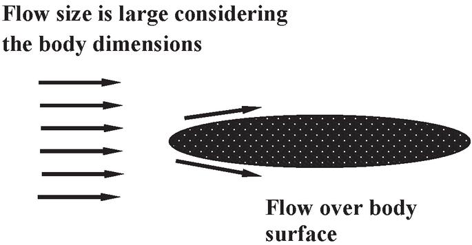
Figure 1 External flow diagram.

A good model has been chosen to show an indirect solution method for several situations involving flow on a flat plate aligned with the flow will be suitably examined in which the physical properties of the fluid are considered constant with the two-dimensional flow in all analytical and numerical solutions, which are detailed in the contribution.

In the energy equation, the dissipation is considered negligible in this work and the solutions examined in the equations, in this case, the energy and the complete Navier-Stokes one are entirely based on the use of the differential equations describing the boundary layers.

3 Problem Definition

3.1 Case of Laminar Flow Over An Isothermal Plate

We consider the problem of the flow of a fluid having a velocity $u_1$ on a flat plate with which a uniform temperature of $T_{\omega }$ is imposed on its total surface which is in front of the body is distinct from that of the fluid $T_1$. The fluid flow situation is clearly shown in Figure 2.

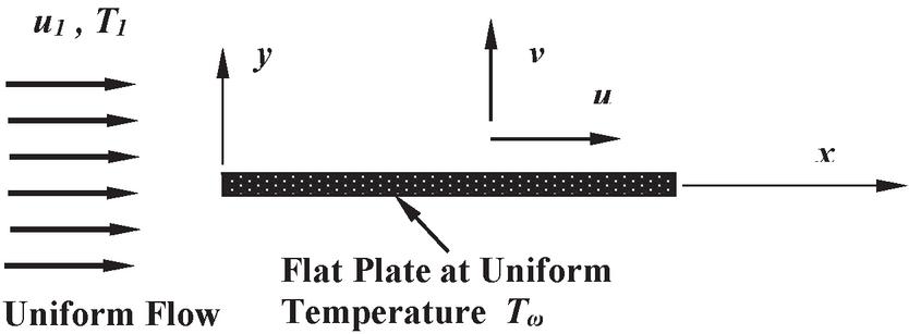
Figure 2 Fluid flow situation over a flat plate.

3.1.1 Mathematical formulation

In order for the boundary layer assumptions to be appropriate, we consider the Reynolds number to be reasonably high and that the flow is quite two-dimensional. In other words, we assume that the plate is extended if taking into account its longitudinal distance. Applying these assumptions, we can write the governing equations describing the problem as:

$$\frac{\partial u}{\partial x}+\frac{\partial v}{\partial y}=0$$	(17)
$$\frac{\partial u}{\partial x}+v\frac{\partial u}{\partial y}=\upsilon \left(\frac{{\partial }^{2}u}{\partial y^2}\right)$$	(18)
$$u\frac{\partial T}{\partial x}+v\frac{\partial T}{\partial y}=\frac{\upsilon }{Pr}\left(\frac{{\partial }^{2}T}{\partial y^2}\right)$$	(19)

Writing these equations shows us that the solution on a flat plate of thickness is zero for an inviscid flow is that the velocity flow is everywhere the same and equivalent to the velocity ’of the free undisturbed flow $u_1$. This means that if the viscosity is negligible, a flat plate aligned with the flow will have no impact on the flow. And as a result of this, everywhere the pressure gradient, dp/dx, is zero.

Logically, to obtain the solution of the boundary layer for the flow on a flat plate, the velocity outside the boundary is assumed equal to $u_l$ and the pressure gradient is neglected everywhere. Commonly, a pressure gradient exists significantly in the case of a real plate of finite thickness but only near the leading edge. Since the equations of the boundary layer are not appropriate in the velocity of the leading edge, in this zone, the longitudinal gradients of temperature and velocity being comparable to the lateral ones and we will neglect this effect here.

In Equation (18), by definition, the kinematic viscosity, $\upsilon$, is expressed by the following relation:

$$\upsilon =\frac{\mu }{\rho }$$

(20)

We also recorded in the insertion of Equation (19) the following notation:

$$\frac{k}{\rho C_p}=\frac{\upsilon }{Pr}$$

(21)

By introducing the following boundary conditions, we can solve the equations going from (17) to (19)

$y=0,u=0,v=0,T=T_{\omega }$
$y\mathrm{large}:u\to u_1,T\to T_1$	(22)

We can see that the Equations (17) and (18) which express the velocity distribution are not related to the temperature because the physical properties of the fluid are already considered constant.

In order to obtain the velocity distribution, the latter two can be solved separately from Equation (19). The temperature distribution of Equation (19) can be obtained therefore, after obtaining the velocity distribution. Therefore, through this distribution, we can determine the heat transfer rate.

3.1.2 Similarity solution

We have used here the similarity solution method which is initially based as an assumption, by considering that all the values of x are similar to the profiles of the boundary layers. In other words and as shown in Figure 3, the velocity profiles for various values of x are all similar.

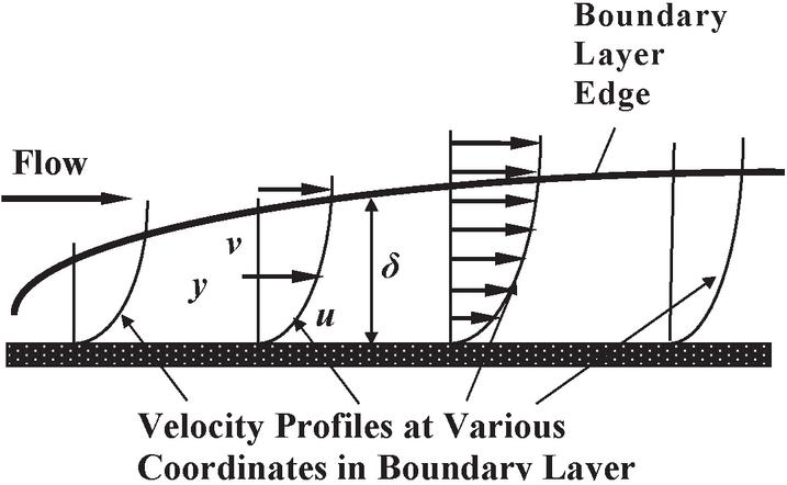
Figure 3 Velocity boundary layer development on a flat plate.

We have assumed that the velocity profile remains geometrically similar and takes the following functional form:

$$\frac{u}{u_1}=\mathrm{function}\left(\frac{y}{\delta }\right)$$

(23)

In this sense, the velocity profiles have been assumed to be similar and the velocity at a certain distance y from the wall and the thickness of the local boundary layer are a function of x.

By applying the assumptions of the boundary layer, we can impose the following form:

$$\frac{\delta }{x}=o\left(\frac{1}{\sqrt{R{e}_x}}\right)$$

(24)

Here, the Reynolds number $R{e}_x$ is a function of x, and x represents the characteristic distance.

Replacing Equation (24) and the expression of Reynolds number ($u_{1}x/\upsilon$) in Equation (23), we get:

${\displaystyle \frac{u}{u_1}}=F\left({\displaystyle \frac{y}{x}}\sqrt{R{e}_x}\right)=F\left(y\sqrt{{\displaystyle \frac{u_1}{\upsilon x}}}\right)$

(25)

We can therefore define new dependent and independent variables, F and $\eta$ respectively in this way:

${\displaystyle \frac{u}{u_1}}$	$=F(\eta )$	(26)
$\eta$	$={\displaystyle \frac{y}{x}}\sqrt{R{e}_x}=y\sqrt{{\displaystyle \frac{u_1}{\upsilon x}}}$	(27)

Where $\eta$ is commonly called the similarity variable.

We can integrate the continuity Equation (17) with respect to y by using the boundary conditions of Equation (22), we get this:

$v=-{\displaystyle {\int }_0^y}{\displaystyle \frac{\partial \eta }{\partial x}}\mathit{d}y=-\sqrt{{\displaystyle \frac{x\upsilon }{u_1}}}{\displaystyle {\int }_0^{\eta }}{u}_1{\displaystyle \frac{dF}{d\eta }}{\displaystyle \frac{\partial \eta }{\partial x}}\mathit{d}\eta$

(28)

By differentiating the similarity variable $\eta$ with respect to x, we can also show that

${\displaystyle \frac{\partial \eta }{\partial x}}=-{\displaystyle \frac{1}{2}}{\displaystyle \frac{y}{x}}\sqrt{{\displaystyle \frac{u_1}{x\upsilon }}}=-{\displaystyle \frac{\eta }{2x}}$

(29)

By substituting in Equation (28), we can draw:

$v={\displaystyle \frac{1}{2}}\sqrt{{\displaystyle \frac{\upsilon }{x{u}_1}}}{\displaystyle {\int }_0^{\eta }}{\displaystyle \frac{dF}{d\eta }}\eta \mathit{d}\eta$

(30)

In order to solve this integral and given its form, it suffices to create another function f which depends on F by the following relation

$$\frac{df}{d\eta }=f^{\prime }=F$$

(31)

By replacing the variables of Equation (31) in Equation (30), we then obtain

$$\frac{v}{u_1}=\frac{1}{2}\sqrt{\frac{\upsilon }{x{u}_1}}(\eta f^{\prime }-f)$$

(32)

In the next step, we consider the moment Equation (18) which will be written in the form

$\left({\displaystyle \frac{u}{u_1}}\right){\displaystyle \frac{\partial (u/u_1)}{\partial \eta }}{\displaystyle \frac{\partial \eta }{\partial x}}+\left({\displaystyle \frac{v}{u_1}}\right){\displaystyle \frac{\partial (u/u_1)}{\partial \eta }}{\displaystyle \frac{\partial \eta }{\partial y}}=\left({\displaystyle \frac{v}{u_1}}\right){\displaystyle \frac{{\partial }^2(u/u_1)}{\partial {\eta }^2}}{\left({\displaystyle \frac{\partial \eta }{\partial y}}\right)}^2$

(33)

However, from Equation (31), we have:

$$\frac{u}{u_1}=f^{\prime }$$

(34)

Using Equation (34) to reduce Equation (33), we can derive the following:

$f^{\prime }{f}^{\prime \prime }\left(-{\displaystyle \frac{1}{2}}{\displaystyle \frac{y}{x}}\sqrt{{\displaystyle \frac{u_1}{x\upsilon }}}\right)+\left[{\displaystyle \frac{1}{2}}\sqrt{{\displaystyle \frac{\upsilon }{x{u}_1}}}(\eta f^{\prime }-f)\right]f^{\prime \prime }\sqrt{{\displaystyle \frac{u_1}{x\eta }}}={\displaystyle \frac{v}{u_1}}{f}^{\prime \prime \prime }\left({\displaystyle \frac{u_1}{x\upsilon }}\right)$

(35)

After the simplifications, we will have:

$$2f^{\prime \prime \prime }+f{f}^{\prime \prime }=0$$

(36)

Finally, Equation (36) can take the following way:

$$2\frac{d^{3}f}{d{\eta }^3}+f\frac{d^{2}f}{d{\eta }^2}=0$$

(37)

Now the hydrodynamic boundary layer problem of finding the velocity profile has been reduced to solving a third-order nonlinear ordinary differential equation.

The boundary conditions provided in Equation (22) will take the following form according to the similarity function terms:

$y=0,u=0,\mathrm{becomes}\eta =0,f^{\prime }=0$
$y=0,v=0,\mathrm{becomes}\eta =0,f=$
$y\mathrm{is}\mathrm{large}:u\to u_1,\mathrm{becomes}\eta \mathrm{is}\mathrm{large},f^{\prime }\to 1$	(38)

We therefore have in terms of similarity variables, one boundary condition imposed on large values of $\eta$ and two boundary conditions at $\eta =0$. Using these boundary conditions, the resolution of Equation (36) has become relatively easy to find.

In order to find the variation of f with $\eta$, we use the first two boundary conditions reported in Equation (38) whose approach is based on the value of $f^{\prime \prime }$ on the wall and then we numerically solve Equation (36).

3.1.3 Numerical solution procedure

To solve this problem, we resorted to the use of an iterative method which is mostly adopted here called Newton’s method. In other words, if $f_{\mathrm{\infty }}^{\prime }$ is the value of $f^{\prime }$ for large $\eta$ and if $f_{\omega }^{\prime \prime }$ is the value of $f^{\prime \prime }$ at $\eta =0$, then an excellent evaluation of $f_{\omega }^{\prime \prime }$ is:

$$f_{\omega }^{\prime \prime }+\frac{f_{\mathrm{\infty }}-1}{d(f_{\mathrm{\infty }}^{\prime })/d(f_{\omega }^{\prime \prime })}$$

The solution methodology requires us to simultaneously write Equation (36) in three first order differential equations like this:

$2h^{\prime }$	$=-0.5fh$
$g^{\prime }$	$=h$
$f^{\prime }$	$=g$

Where this system of equation is subject to the following boundary conditions

$$\eta =0,g=0;\eta =0,f=0;\eta \mathrm{large},g\to 1$$

The solution method therefore, includes penetrating the value of $\eta$ to zero and then integrating the system of equations.

Then, we exploited Newton’s method in order to progress gradually towards h at $\eta =0$ which gives $g\to 1$ for $\eta$ large. As an application, the value of $d(f_{\mathrm{\infty }}^{\prime })/d(f_{\omega }^{\prime \prime })$ is arrived at by obtaining $f_{\mathrm{\infty }}^{\prime }$ using a singular value of $f_{\omega }^{\prime }$ and then incrementally $f_{\omega }^{\prime }$ by a small amount, then by obtaining a new value of $f_{\mathrm{\infty }}^{\prime }$ and then using for the derivative by a finite difference technique.

The thermal boundary layer develops on an isothermal flat plate if surface temperatures differ and the free fluid stream, just as the velocity boundary layer develops in the presence of fluid flow over a surface (Figure 4).

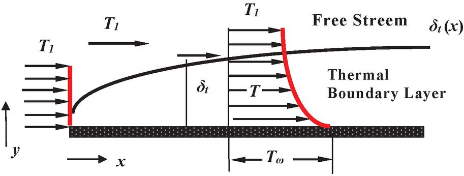
Figure 4 Thermal boundary layer development on an isothermal flat plate.

So far we have determined the velocity profile, now our concern is focused on finding the temperature field from the previous Equation (19). In the present situation since the temperature of the wall is quite uniform, we assume that the velocity profile is similar to that of the temperature. Therefore, we introduce the following dimensionless variable of the temperature:

$\theta ={\displaystyle \frac{T_{\omega }-T}{T_{\omega }-T_1}}$

(39)

We therefore consider that the variable $\theta$ is related only to that of similarity, $\eta$, since the thickness of the thermal boundary layer is equivalent to $x/\sqrt{R{e}_x}$.

The energy Equation (19) will take the following form since $T_1$ and $T_{\omega }$ are constants

$u{\displaystyle \frac{\partial \theta }{\partial x}}+v{\displaystyle \frac{\partial \theta }{\partial y}}={\displaystyle \frac{\upsilon }{Pr}}{\displaystyle \frac{{\partial }^2\theta }{\partial y^2}}$

(40)

And in this case, the boundary conditions will be:

$y=0:\theta =0$
$y\mathrm{large}:\theta \to 1$	(41)

Consider that $\theta$ varies as a function of $\eta$ and after making the changes and derivatives in the Equation (40), we will have:

$f^{\prime }{\displaystyle \frac{d\theta }{d\eta }}{\displaystyle \frac{\partial \eta }{\partial x}}+\left[{\displaystyle \frac{1}{2}}\sqrt{{\displaystyle \frac{\upsilon }{x{u}_1}}}(\eta f^{\prime }-f)\right]{\displaystyle \frac{d\theta }{d\eta }}{\displaystyle \frac{\partial \eta }{\partial y}}={\displaystyle \frac{1}{Pr}}{\displaystyle \frac{v}{u_1}}{\displaystyle \frac{{\partial }^2\theta }{\partial {\eta }^2}}{\left[{\displaystyle \frac{\partial \eta }{\partial y}}\right]}^2$

(42)

By making the necessary simplifications, Equation (42) reduces to

$${\theta }^{\prime \prime }+\frac{Pr}{2}{\theta }^{\prime }f=0$$

(43)

Where the latter is subject to the following appropriate boundary conditions:

$\eta =0:\theta =0$
$\eta \mathit{\hspace{1em}}\mathrm{large}:\theta \to 1$	(44)

By confirming the hypothesis of similarity of the temperature field, and as we had done for the case of velocity, the partial differential equation governing the temperature distribution was reduced to a single ordinary differential equation.

Using the boundary conditions of Equation (44), we can solve Equation (43) whose solution procedure is now easier to follow and it will be written as follows:

${\displaystyle \frac{1}{{\theta }^{\prime }}}{\displaystyle \frac{d}{d\eta }}{\theta }^{\prime }=-{\displaystyle \frac{Pr}{2}}f$

(45)

By integrating this equation, we get

$${\theta }^{\prime }=c_1\exp \left[-\frac{Pr}{2}{\int }_0^{\eta }f\mathit{d}\eta \right]$$

(46)

Where c1 represents the constant of integration to be determined which then gives.

The integration of Equation (46) will guide us to:

$\theta =c_1{\displaystyle {\int }_0^{\eta }}\left[\exp \left(-{\displaystyle \frac{Pr}{2}}{\displaystyle {\int }_0^{\eta }}f\mathit{d}\eta \right)\right]d\eta +c_2$

(47)

A second integration constant $c_2$ has appeared in Equation (47) and is equal to zero because in accordance with the boundary conditions of Equation (44) we have $(\eta =0$; $\theta =0$). Moreover, the constant $c_1$ is obtained by using the second boundary conditions of Equation (44), and it will take the following expression:

$c_1=1/{\displaystyle {\int }_0^{\mathrm{\infty }}}\left[\exp \left(-Pr{\displaystyle {\int }_0^{\eta }}f\mathit{d}\eta \right)\right]d\eta$

(48)

By taking into account the null value of $c_2$ and then replacing Equation (48) in Equation (47), we get the final solution of $\theta$ as:

$$\theta =\frac{{\int }_0^{\eta }\left[\exp \left(-\frac{Pr}{2}{\int }_0^{\eta }f\mathit{d}\eta \right)\right]d\eta }{{\int }_0^{\mathrm{\infty }}\left[\exp \left(-\frac{Pr}{2}{\int }_0^{\eta }f\mathit{d}\eta \right)\right]d\eta }$$

(49)

Knowing the function f determined by the speed, we can easily determine $\theta$ as a function of $\eta$ and Equation (36) is written as:

$$\frac{f^{\prime \prime \prime }}{f^{\prime \prime }}=-\frac{f}{2}$$

(50)

The integration of this tends towards

$${\log }_{\mathrm{e}}{f}^{\prime \prime }=-\frac{1}{2}{\int }_0^{\eta }f\mathit{d}\eta +\mathrm{constant}$$

Whence

$$\exp \left[-\frac{1}{2}{\int }_0^{\eta }f\mathit{d}\eta \right]=\frac{f^{\prime \prime }}{c_3}$$

(51)

Hence $c_3$ is a constant. We integrate this equation, we will have

${\displaystyle {\int }_0^{\eta }}\exp \left[-Pr{\displaystyle {\int }_0^{\eta }}f\mathit{d}\eta \right]\mathit{d}\eta ={\displaystyle {\int }_0^{\eta }}{\left({\displaystyle \frac{f^{\prime \prime }}{c_3}}\right)}^{Pr}\mathit{d}\eta ={\displaystyle \frac{1}{c_3^{Pr}}}{\displaystyle {\int }_0^{\eta }}{(f^{\prime \prime })}^{Pr}\mathit{d}\eta$

Introducing these important results into Equation (49) entails

$\theta$	$={\displaystyle \frac{\left[{\int }_0^{\eta }{(f^{\prime \prime })}^{Pr}\mathit{d}\eta \right]}{\left[{\int }_0^{\mathrm{\infty }}{(f^{\prime \prime })}^{Pr}\mathit{d}\eta \right]}}$
	$={\displaystyle \frac{\left[{\int }_0^{\mathrm{\infty }}{(f^{\prime \prime })}^{Pr}\mathit{d}\eta -{\int }_{\eta }^{\mathrm{\infty }}{(f^{\prime \prime })}^{Pr}\mathit{d}\eta \right]}{\left[{\int }_0^{\mathrm{\infty }}{(f^{\prime \prime })}^{Pr}\mathit{d}\eta \right]}}$
	$=1-{\displaystyle \frac{\left[{\int }_{\eta }^{\mathrm{\infty }}{(f^{\prime \prime })}^{Pr}\mathit{d}\eta \right]}{\left[{\int }_0^{\mathrm{\infty }}{(f^{\prime \prime })}^{Pr}\mathit{d}\eta \right]}}$	(53)

Thus, for any selected value of the Prandtl number Pr, we can obtain the prediction of the dimensionless temperature $\theta$ as a function of the similarity variable $\eta$.

Since the velocity gives us the variation of $f^{\prime \prime }$ with $\eta$, we can easily find by this, the variation of $\theta$ with $\eta$. For large high values of $\eta$, outside the boundary layer, the value of $f^{\prime \prime }$, equal to $d(u/u_l)/d\eta$ is remarkable tends towards zero.

In order to obtain the similarity contours, we have developed a program in FORTRAN language to solve our problem on the prediction of the velocity field and that of temperature at the same time. We used the Runge-Kutta method to solve the system of equations analyzing the velocity profile. Figure 5 represents the schematic flowchart of the operation of the FORTRAN code (inputs/outputs) and converges to the numerical solution of the problem.

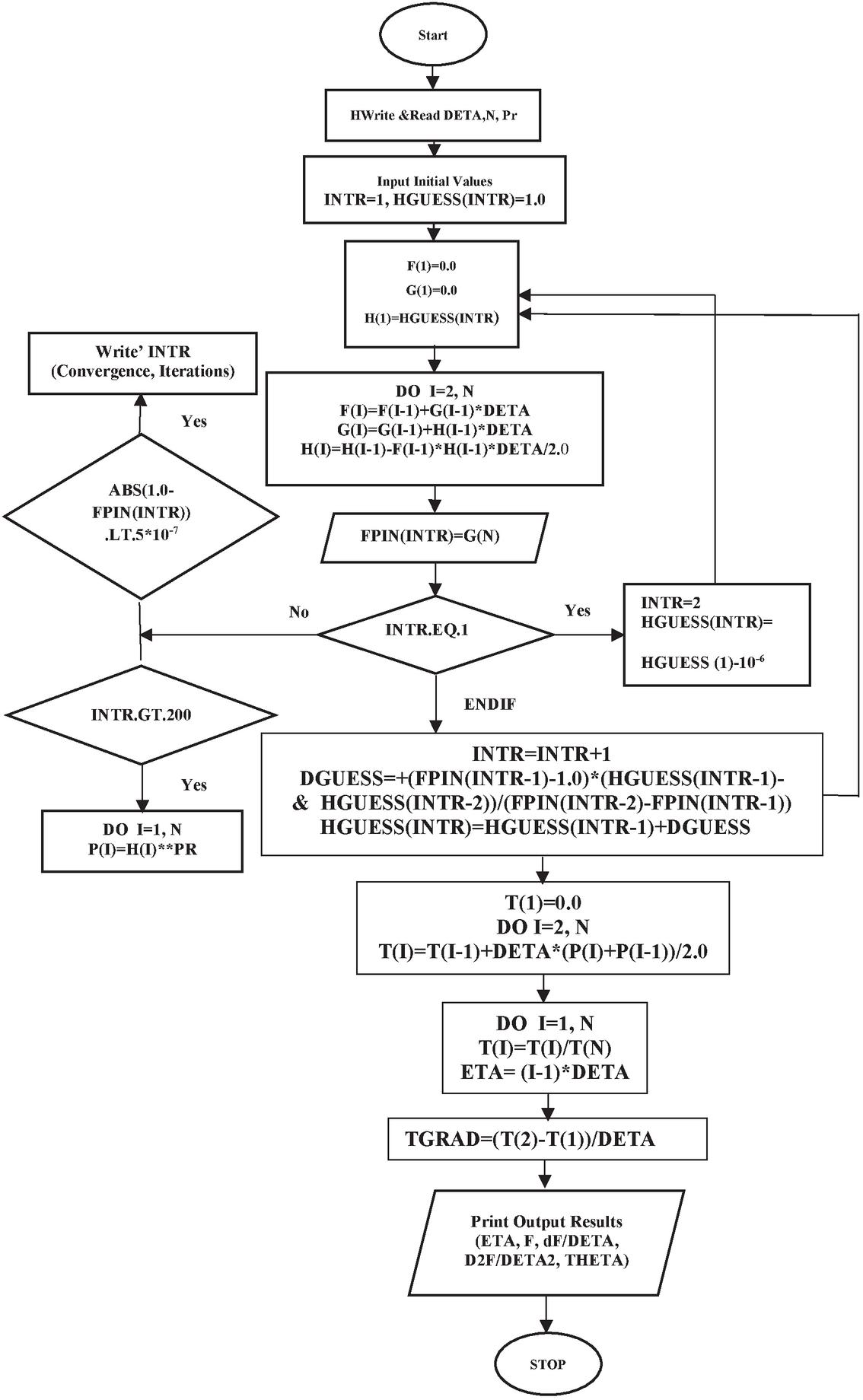
Figure 5 Flowchart of the FORTRAN code giving similarity solution results for laminar boundary layer flow over an isothermal flat plate.

3.1.4 Runge-Kutta 4th order rule for differential equation

The fourth-order Runge – Kutta method is used for solving ordinary differential equations (ODE). It uses dy/dx function for x and y, and also needs the initial value of y, i.e. y(0). It finds the approximate value of y for given x. The Runge-Kutta method RK4 requires 4 evaluations of f and four coefficients $k_1$, $k_2$, $k_3$, and $k_4$. The following formula $[y_{n+1}=y_n+h/6(k_1+2k_2+2k_3+k_4)]$ is used to compute next value $y_{n+1}$ from previous value $y_n$. The value of n are $0,1,2,3,\mathrm{\dots }(x-x_0)/h$ where $h$ is step height and $x_{n+1}=x_n+h$ For solving ODE.

Figure 6 shows the flow chart representing the code programmed for the solution of the ODE using Runge–Kutta 4th order method.

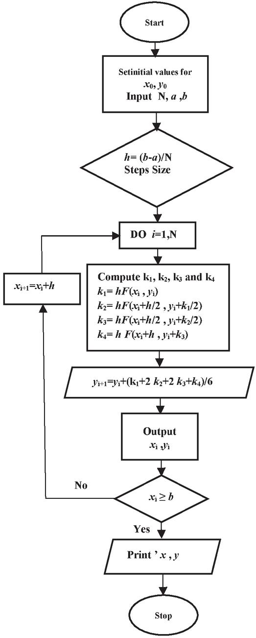
Figure 6 Flowchart of the Runge–Kutta 4th order method in FORTRAN.

3.2 Case of Laminar Flow Over Flat Plates with Other Thermal Boundary Conditions

3.2.1 Mathematical formulation and similarity solution

We have previously discussed the similarity solution of a plate subjected to a uniform surface temperature, of which we had:

$$T_{\omega }-T_1=\mathrm{constant}$$

Moreover, other solutions of similarity with other thermal boundary conditions can be achieved for a flat plate by holding that its temperature is variable as a function of the abscissa x. The boundary conditions on the temperature do not influence the resolutions of the velocity field and are considered identical to those for the uniform temperature and we consider here:

$$T_{\omega }=T_1+C{x}^n$$

From where:

$$T_{\omega }-T_1=C{x}^n$$

(54)

Where C and n are also constants.

The nondimensionalization of the temperature used here is defined by:

$$\theta =\frac{T_{\omega }-T}{T_{\omega }-T_1}=1-\frac{T-T_1}{T_{\omega }-T_1}$$

(55)

And again, since we have assumed that $\theta$ is independent of the similarity variable, $\eta$.

$T_{\omega }-T_1$ is variable in this case as a function of x because of what we have:

$$T-T_1=(1-\theta )(T_{\omega }-T_1)$$

We can therefore write the energy Equation (19) as a function of $\theta$ as

$-u{\displaystyle \frac{\partial }{\partial x}}\left[\left(1-\theta \right)\left(T_{\omega }-T_1\right)\right]+v{\displaystyle \frac{\partial \theta }{\partial y}}(T_{\omega }-T_1)=\left[{\displaystyle \frac{\upsilon }{Pr}}\right]{\displaystyle \frac{{\partial }^2\theta }{\partial y^2}}(T_{\omega }-T_1)$

And the boundary conditions will become

$y=0:\theta =0$
$y\mathrm{large}:\theta \to 1$	(57)

Equation (72) will take the following form and this after having used the relations of the derivatives of the velocity obtained later

$f^{\prime }{\displaystyle \frac{d\theta }{d\eta }}{\displaystyle \frac{\partial \eta }{\partial x}}-{\displaystyle \frac{\eta f^{\prime }\left(1-\theta \right)}{x}}+\left[{\displaystyle \frac{1}{2}}\sqrt{{\displaystyle \frac{\upsilon }{u_{1}x}}}\left(\eta f^{\prime }-f\right)\right]{\displaystyle \frac{d\theta }{d\eta }}{\displaystyle \frac{\partial \eta }{\partial y}}$
$\mathrm{\hspace{1em}\hspace{1em}}={\displaystyle \frac{1}{Pr}}{\displaystyle \frac{\upsilon }{u_1}}{\displaystyle \frac{d^2\theta }{d{\eta }^2}}{\left[{\displaystyle \frac{\partial \eta }{\partial y}}\right]}^2$	(58)

After simplifications, we obtain the following equation:

${\theta }^{\prime \prime }+\eta {\mathit{Prf}}^{\prime }(1-\theta )+{\displaystyle \frac{Pr}{2}}{\theta }^{\prime }f=0$

(59)

Subject to the boundary conditions which take the following form:

$\eta =0:\theta =0$
$\eta \mathrm{large}:\theta \to 1$	(60)

As we had previously found, the governing partial differential equation for the temperature field was transferred to an ordinary differential equation by introducing the similarity variables. The assumption of the temperature contours which are identical was thus verified.

The dimensionless temperature variation $\theta$ as a function of the similarity variable $\eta$ can be predicted by solving the equation in question for all selected values of Pr and $\eta$.

Thanks to a FORTRAN program that we have well elaborated by all the required data, we were able to reach the solution results of the speed profile and again the same method to solve Equation (59).

The rate of heat transfer to the wall is known by its formula:

$$q_{\omega }=-{k\frac{\partial T}{\partial y}|}_{y=0}$$

(61)

Finally, and after using Equation (55), we therefore have:

$$\frac{q_{\omega }x}{k(T_{\omega }-T_{1)}}={{\theta }^{\prime }|}_{\eta =0}\sqrt{R{e}_x}$$

(62)

For each imposed value of Pr and $\eta$, ${{\theta }^{\prime }|}_{\eta =0}$ will take a characteristic value. It subsequently appears the proportionality of $q_{\omega }$ to $(T_{\omega }-T_1)/x^{0.5}$. However, in the case where n takes the value of 0.5, this indeed corresponds to the uniformity of heat flux on the surface of the plate.

In other words, for a flow on a flat plate that is subjected to a heat flux of uniform area, the similarity solution of the governing equation is always exists.

4 Results and Discussion

4.1 Flat Plate in Laminar Flow

Subsequently, we can find the evolution of $f$ and $f^{\prime }$, as a function of $\eta$ whose curve is well illustrated in Figure 7. Generally, the fluid velocity is zero at the plate surface and increases gradually away from the plate toward the free stream value satisfying the boundary conditions. We can see that the desired speed profile is in good agreement with the experimental investigations observed. Although reducing the two original partial differential equations governing the velocity components, u and v, into a single ordinary differential equation gives us a reliable justification for the hypothesis of similar velocity contours. Physically in the boundary layer, there is no distinct “edge” and for it to have dominant viscosity effects there must be some measure of distance from the wall.

For this purpose, it is practically to determine the thickness of the boundary layer ${\delta }_u$, also the distance from the wall at which u reaches at less than 1% of the velocity of the free stream, i.e., to define $\delta$ as the value of y at which $u=0.99u_l$. According to the result schematized in Figure 7, we can see that $u=0.99u_1$. This means that, when $\eta =5$ then $f^{\prime }=0.99$ which means by the definition of $\eta$ that the thickness of the boundary layer ${\delta }_u$ can be evaluated by:

$${\delta }_u\sqrt{\frac{u_1}{\upsilon x}}=5$$

From where

$$\frac{{\delta }_u}{x}=\frac{5}{\sqrt{R{e}_x}}$$

(63)

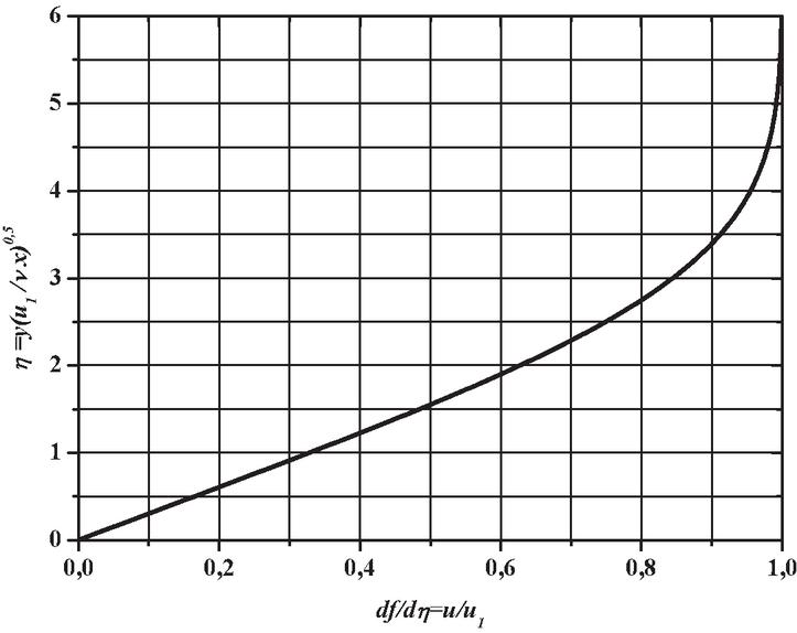
Figure 7 Velocity profile versus the similarity variable for the boundary layer on a flat plate.

Table 1 presents the computational results of the numerical simulation with a fixed value $Pr=1$, for the function $f(\eta$) and its derivatives $(f^{\prime }(\eta ),f^{\prime \prime }(\eta ))$ and dimensionless temperature $\theta (\eta )$. Selected results are presented, from which useful information may be extracted. The x-component velocity distribution from the third column of the table is plotted in Figure 8(a). For different values of the Prandtl number; representative temperature distributions for Pr $=$ 0.7,1,3, and 10 are shown in Figure 8(b). Thermal effects penetrate farther into the velocity boundary layer with decreasing Prandtl number and transcend the velocity boundary layer for $Pr<1$. An important consequence of this solution is quite remarkable, for Pr $=$ 0.6.

Table 1 Computational table showing the function $f(\eta )$, its derivatives $f^{\prime }(\eta )$, $f^{\prime \prime }(\eta )$ and the dimensionless temperature results $\theta (\eta )$

$\eta$	$f(\eta )$	$f^{\prime }(\eta )$	$f^{\prime \prime }(\eta )$	$\theta (\eta )$
0.000000	0.000000	0.000000	0.330308	0.000000
0.010000	0.000000	0.003303	0.330308	0.003309
0.020000	0.000033	0.006606	0.330308	0.006617
0.030000	0.000099	0.009909	0.330308	0.009926
0.040000	0.000198	0.013212	0.330308	0.013234
0.050000	0.000330	0.016515	0.330308	0.016543
0.060000	0.000495	0.019818	0.330307	0.019851
0.070000	0.000694	0.023122	0.330306	0.023160
0.080000	0.000925	0.026425	0.330305	0.026468
0.090000	0.001189	0.029728	0.330304	0.029777
0.100000	0.001486	0.033031	0.330302	0.033085
0.200000	0.006276	0.066059	0.330246	0.066168
0.300000	0.014368	0.099078	0.330087	0.099240
0.400000	0.025760	0.132074	0.329770	0.132289
0.500000	0.040451	0.165029	0.329241	0.165296
0.600000	0.058435	0.197919	0.328447	0.198237
0.700000	0.079704	0.230717	0.327336	0.231083
0.800000	0.104247	0.263387	0.325859	0.263800
0.900000	0.132050	0.295892	0.323966	0.296349
1.000000	0.163094	0.328186	0.321612	0.328685
2.000000	0.644028	0.627550	0.266425	0.628267
3.000000	1.387772	0.844516	0.161869	0.845069
4.000000	2.295155	0.954988	0.064627	0.955236
5.000000	3.272244	0.991467	0.015973	0.991532
6.000000	4.268533	0.998976	0.002388	0.998986

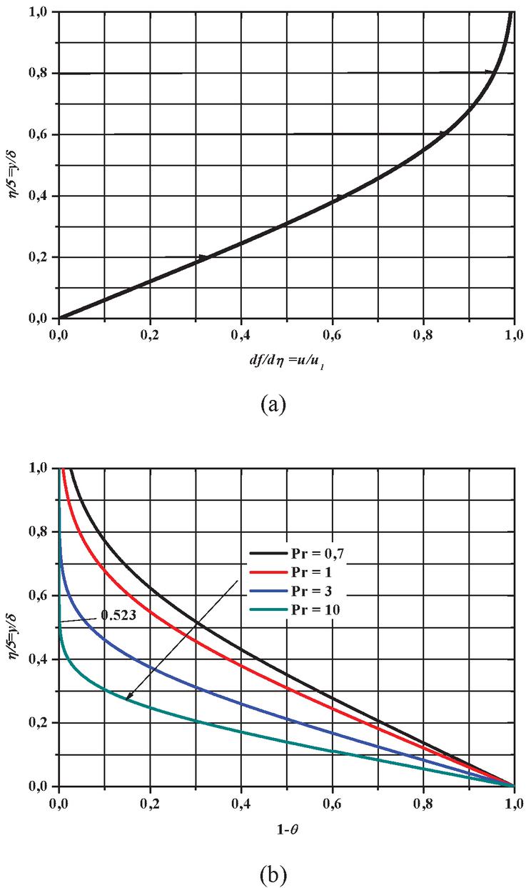
Figure 8 Similarity solution for laminar flow over an isothermal flat plate. (a) x-component of the velocity. (b) Temperature distributions for $Pr=0.7$, 1, 3, and 10.

Figure 9 depicts the non-effect of Prandtl number on the fluid velocity profile. In other words, the fluid velocity distribution is independent of the Prandtl number values. This result is quite normal because the previous differential equations describing the velocity field do not contain any trace of this number.

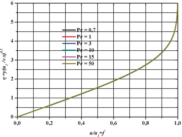
Figure 9 Independence of the Prandtl number on the velocity profile in the flat plate boundary layer.

In our simulation, the function $f(\eta )$ was evaluated for the laminar boundary layer along with a flat plate with zero incidence. Table 2 shows the comparison between the dimensionless velocity values obtained by Blasius [1] and those of the present method. The velocity profile is obtained in dimensionless form by plotting $u/u_1$ as a function of the numerical values grouped together in this table

Table 2 Comparison of $f^{\prime }(\eta )$ between our numerical results and Blasius’s results with Pr $=$ 0.7

$\eta$	$df(\eta )/d\eta$ Present Method	$df(\eta )/d\eta$ Blasius [1]
0	0	0
0.5	0.165029	0.1659
1	0.328186	0.3298
1.5	0.48471	0.4868
2	0.62755	0.6298
2.5	0.749263	0.7513
3	0.844516	0.846
3.5	0.912053	0.913
4	0.954988	0.9555
4.5	0.979284	0.9795
5	0.991467	0.9915
5.5	0.996865	0.9969
6	0.998976	0.999

The results of the numerical investigation with the Blasius solution are presented in Figure 10. This result clearly shows satisfactory agreements with the results of Blasius’ solution.

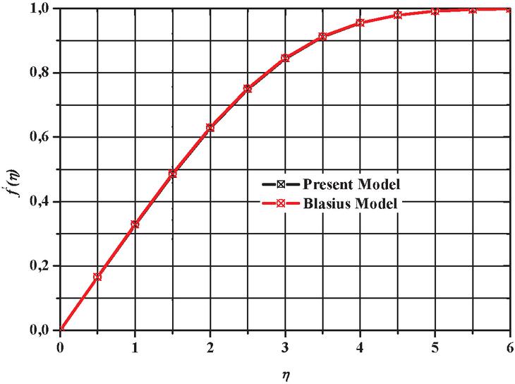
Figure 10 Comparison of the present model with Blasius [1] for the derivative function $f^{\prime }(\eta )$.

Thanks to this FORTRAN program, some specific variations of the dimensionless temperature $\theta$ as a function of the variable $\eta$ for different values of Pr have been plotted in Figure 11. The Prandtl number relates the rates of diffusion of heat and momentum. Prandtl number signifies the thickness of the thermal boundary layer and thickness of the hydrodynamic boundary layer, depending on whether it is equal to one, or more than one, or less than one. If it is equal to one, it signifies that the thickness of the thermal boundary layer is equal to that of the velocity boundary layer. The buoyancy force exerted by a fluid on a body is equal to the weight of the fluid displaced by the body and it is due to the increase of pressure with depth in a fluid. From Figure 11 we observed that a lower temperature and thinner thermal boundary layer thickness correspond to an increase in the Prandtl number. An enhancement in the Prandtl number implies to higher momentum diffusivity and lower thermal diffusivity. The rise in temperature allows the fluid to increase the velocity profile due to the effect of buoyancy; the effects of the heat sink on velocity and temperature profiles play oppositely. This in fact shows the thinning of the thermal boundary layer, which is mainly due to the fact that the buoyancy force improves the fluid velocity and increases the boundary layer thickness with the decrease in the value of Pr. As is well known, the presence of buoyancy enhances the mixing and exchange of the fluid between the near-wall region and the region outside in the unstable boundary layer flow. Hence, convective surface heat transfer enhances thermal diffusion while an increase in the Prandtl number and the intensity of the buoyancy force slows down the rate of thermal diffusion within the boundary layer. For a value of the Prandtl number is equal to 1, the profile is similar to that represented by the variation of $f^{\prime }$ with $\eta$ which was illustrated in Figure 7.

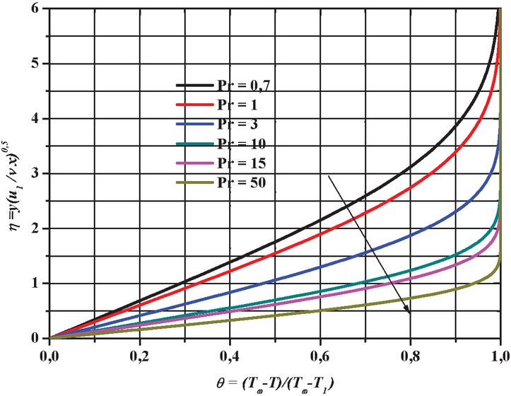
Figure 11 Dimensionless temperature profile $\theta$ versus similarity variable, $\eta$, for different values of Prandtl number Pr for boundary layer on a flat plate.

Figure 12 depicts the three dimensionless temperature distribution $\theta$ versus $\eta$ and $f^{\prime }$ in steady-state heat transfer over a flat plate model.

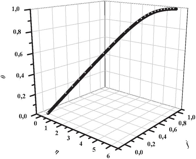
Figure 12 3D Contour plot of dimensionless temperature $\theta$ versus. the similarity variable $\eta$ and the velocity profile $u/u_1$.

It will be checked according to the results given in Figure 11, if the thickness of the thermal boundary layer ${\delta }_T$ is determined similarly to the thickness of the velocity boundary layer as being the wall spacing over which $\theta$ tends to 0.099, from where it reaches less than 1% of its free stream value, so we have

$$\frac{{\delta }_T}{x}=\frac{\mathrm{\Delta }(Pr)}{\sqrt{R{e}_x}}$$

However

$$\frac{{\delta }_u}{x}=\frac{5}{\sqrt{R{e}_x}}$$

This leads to the following writing:

$$\frac{{\delta }_T}{{\delta }_u}=\mathrm{\Delta }(\mathrm{Pr})$$

Figure 13 shows the variation of dimensionless temperature $\theta$ versus dimensionless velocity profile $u/u_1$ for different Prandtl numbers (Pr). However, in this figure, an increase in Prandtl Pr number decreases skin friction but also increases the rate of heat transfer to the plate surface. This is attributed to the fact that as the Prandtl number decrease, the thermal boundary layer thickness increases, causing a reduction in the temperature gradient at the surface of the plate.

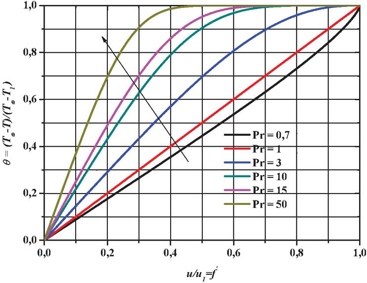
Figure 13 Variation of temperature profile function $\theta$ with respect to the velocity profile $u/u_1$ for several values of Pr.

We can say by this that the relation of the two boundary layer thicknesses is related only to the Prandtl number. According to the results shown in Figure 11, as the Prandtl number is less than one, the thermal boundary layer is thicker than the speed boundary layer and when Pr is greater than one, it is thinner than the speed boundary.

The rate of heat transfer to the wall can be expressed as:

$$q_{\omega }=-{k\frac{\partial T}{\partial y}|}_{y=0}$$

(64)

Using Equation (39), we can derive this

${\displaystyle \frac{q_{\omega }}{k(T_{\omega }-T_1)}}$

$={{\displaystyle \frac{\partial \theta }{\partial y}}|}_{y=0}={{\displaystyle \frac{d\theta }{d\eta }}|}_{\eta =0}{\displaystyle \frac{\partial \eta }{\partial y}}$

(65)

This gives

$$\frac{q_{\omega }x}{k(T_{\omega }-T_1)}={{\theta }^{\prime }|}_{\eta =0}\sqrt{R{e}_x}$$

(66)

We obtain

$$N{u}_x={{\theta }^{\prime }|}_{\eta =0}\sqrt{R{e}_x}$$

(67)

Obviously, Re and Nu are respectively the local Reynolds and Nusselt numbers based on the x-coordinate. Because, for known Pr, $\theta$ is dependent on $\eta$, ${{\theta }^{\prime }|}_{\eta =0}$ is only related to Pr and we can get it using the solution of $\theta$ as a function of $\eta$. We can define:

$$A(\mathrm{Pr})={{\theta }^{\prime }|}_{\eta =0}$$

(68)

We can deduce from Equation (67) the following:

$$N{u}_x=A(\mathrm{Pr})\sqrt{R{e}_x}$$

(69)

Our calculation results of the function A for different Pr values are obtained and summarized in Table 3.

Table 3 Estimated values of A as a function of the values of the Prandtl number

$Pr$	$A={{\theta }^{\prime }|}_{\eta }=0$	0.332 $P{r}^{1/3}$
0.6	0.276	0.280
0.7	0.293	0.295
0.8	0.307	0.308
0.9	0.320	0.321
1.0	0.332	0.332
1.1	0.344	0.343
7.0	0.645	0.635
10.0	0.730	0.715
15.0	0.835	0.819

Subsequently, integration on the whole plate is essential to acquire the whole rate of heat transfer. Moreover, after having gained the compact approximate relation A, it is compared to the function 0.332Pr${}^{\mathrm{1}\mathrm{/}\mathrm{3}}$. Figure 14 represents this comparison for various Prandtl Numbers: 0.6, 0.7,…and 15.

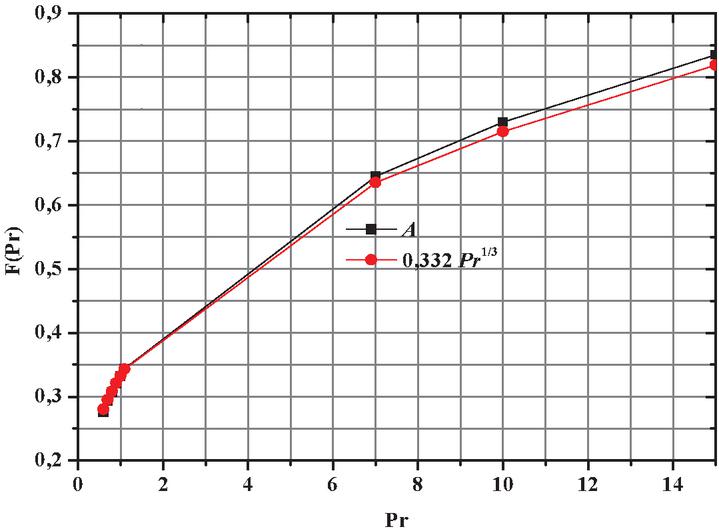
Figure 14 Comparison in order to roughly estimate the function of A.

From the results cited in the table, we can visibly see that the values of function A vary in the vicinity of $P{r}^{1/3}$ and, we can consider that the results given in the table of A are very similar and close to those of the second column, we can get the following approximate expression:

$$A=0.332{\mathrm{Pr}}^{1/3}$$

(70)

For values greater than 1 or very different from those in the table, the calculation error of the approximate equation is remarkable and very important. Presently, in practice, our thermal problem is possibly related to the rate of total heat transfer starting with the whole surface than to the rate of local heat transfer. We now consider that from a plate of length L, there is a total heat transfer rate. We assume by the hypothesis that the flow is two-dimensional since the unit width of the plate is considered here. The total heat transfer rate per unit of width will obviously depend on the local heat transfer rate, by:

$$Q_{\omega }={\int }_0^L{q}_{\omega }\mathit{d}x$$

(71)

Nevertheless, Equation (66) inevitably presents the local heat transfer rate then:

$$q_{\omega }=Ak(T_{\omega }-T_1)\sqrt{\frac{u_1}{x\upsilon }}$$

(72)

By replacing and doing the integral, Equation (71) becomes

$$Q_{\omega }=2Ak(T_{\omega }-T_1)\sqrt{\frac{u_{1}L}{\upsilon }}$$

(73)

If the entire plate has an average heat transfer coefficient $\overline{h}$, its expression can be defined as

$$\overline{h}=\frac{Q_{\omega }}{L(T_{\omega }-T_1)}$$

(74)

Therefore, given that for the plate its unit width is taken into account, Equation (73) deduces:

$$\overline{h}=\frac{2Ak}{L}\sqrt{\frac{u_{1}L}{\upsilon }}$$

(75)

So, for the whole plate, the relation of the mean Nusselt number $N{u}_L$ can be formulated as:

$$N{u}_L=2ARe_L{}^{1/2}$$

(76)

Where $R{e}_L$ is the Reynolds number based on the length of the plate, $L$.

In what follows, we will see that for the entire surface of the plate, the average transfer rate is twice the local heat transfer rate at the end of the plate $(x=L)$.

From the approximate expression of the function A given in Equation (70), the formulas for local and average Nusselt numbers are therefore:

$N{u}_x$	$=0.332{\mathrm{Pr}}^{1/3}Re_x{}^{1/2}$	(77)
$N{u}_x$	$=0.664{\mathrm{Pr}}^{1/3}Re_L{}^{1/2}$	(78)

These correlation formulas provide the fruit of results which are completely in agreement with the experimental investigations.

4.2 Flat Plate in Laminar Flow with Other Thermal Boundary Conditions

The results of the numerical solutions for $f(\eta )$ and its derivatives, as well as the dimensionless temperature $\theta$ are given in Table 4(a-b-c-d) for fixed Prandtl numbers of 0.7 and by varying the exponent n (0, 0.5, 1, 1.5). We can notice according to the results gathered in this table that for a fixed Prandtl number, both $f^{\prime \prime }(\eta )$ and $\theta (\eta )$ increase as an exponent n increases.

Table 4 Computational results outputs of the FORTRAN code

(a) $n=0$. $Pr=0.7$
$\eta$	$f(\eta )$	$f^{\prime }(\eta )$	$f^{\prime \prime }(\eta )$	$\theta (\eta )$
0.000000	0.000000	0.000000	0.292681	0.000000
0.010000	0.000017	0.003321	0.292681	0.002927
0.020000	0.000066	0.006641	0.292681	0.005854
0.030000	0.000149	0.009962	0.292681	0.008780
0.040000	0.000266	0.013282	0.292681	0.011707
0.050000	0.000415	0.016603	0.292681	0.014634
0.060000	0.000598	0.019923	0.292680	0.017561
0.070000	0.000814	0.023244	0.292679	0.020488
0.080000	0.001063	0.026565	0.292679	0.023414
0.090000	0.001345	0.029885	0.292677	0.026341
0.100000	0.001660	0.033206	0.292676	0.029268
0.200000	0.006641	0.066408	0.292636	0.058534
0.300000	0.014941	0.099599	0.292528	0.087793
0.400000	0.026560	0.132764	0.292319	0.117036
0.500000	0.041493	0.165885	0.291974	0.146252
0.600000	0.059735	0.198937	0.291460	0.175425
0.700000	0.081277	0.231890	0.290744	0.204537
0.800000	0.106108	0.264709	0.289795	0.233566
0.900000	0.134213	0.297354	0.288582	0.262487
1.000000	0.165572	0.329780	0.287074	0.291273
2.000000	0.650025	0.629766	0.251085	0.563780
3.000000	1.396810	0.846045	0.176605	0.780110
4.000000	2.305748	0.955519	0.092679	0.913756
5.000000	3.283276	0.991542	0.034886	0.974595
6.000000	4.279623	0.998973	0.009289	0.994495
(b) $n=0.5$. $Pr=0.7$
$\eta$	$f(\eta )$	$f^{\prime }(\eta )$	$f^{\prime \prime }(\eta )$	$\theta (\eta )$
0.000000	0.000000	0.000000	0.405895	0.000000
0.010000	0.000017	0.003321	0.405889	0.004059
0.020000	0.000066	0.006641	0.405872	0.008118
0.030000	0.000149	0.009962	0.405843	0.012176
0.040000	0.000266	0.013282	0.405803	0.016235
0.050000	0.000415	0.016603	0.405751	0.020292
0.060000	0.000598	0.019923	0.405688	0.024349
0.070000	0.000814	0.023244	0.405613	0.028406
0.080000	0.001063	0.026565	0.405527	0.032462
0.090000	0.001345	0.029885	0.405430	0.036516
0.100000	0.001660	0.033206	0.405322	0.040570
$\eta$	$f(\eta )$	$f^{\prime }(\eta )$	$f^{\prime \prime }(\eta )$	$\theta (\eta )$
0.200000	0.006641	0.066408	0.403634	0.081027
0.300000	0.014941	0.099599	0.400878	0.121261
0.400000	0.026560	0.132764	0.397104	0.161168
0.500000	0.041493	0.165885	0.392361	0.200649
0.600000	0.059735	0.198937	0.386699	0.239610
0.700000	0.081277	0.231890	0.380172	0.277960
0.800000	0.106108	0.264709	0.372834	0.315617
0.810000	0.108772	0.267982	0.372058	0.319342
0.900000	0.134213	0.297354	0.364741	0.352502
1.000000	0.165572	0.329780	0.355949	0.388542
2.000000	0.650025	0.629766	0.243290	0.690851
3.000000	1.396810	0.846045	0.128082	0.874506
4.000000	2.305748	0.955519	0.050915	0.960172
5.000000	3.283276	0.991542	0.015041	0.990329
6.000000	4.279623	0.998973	0.003260	0.998232
(c) $n=1$. $Pr=0.7$
$\eta$	$f(\eta )$	$f^{\prime }(\eta )$	$f^{\prime \prime }(\eta )$	$\theta (\eta )$
0.000000	0.000000	0.000000	0.480339	0.000000
0.010000	0.000017	0.003321	0.480327	0.004803
0.020000	0.000066	0.006641	0.480293	0.009606
0.030000	0.000149	0.009962	0.480235	0.014409
0.040000	0.000266	0.013282	0.480155	0.019211
0.050000	0.000415	0.016603	0.480052	0.024012
0.060000	0.000598	0.019923	0.479927	0.028812
0.070000	0.000814	0.023244	0.479779	0.033610
0.080000	0.001063	0.026565	0.479609	0.038407
0.090000	0.001345	0.029885	0.479418	0.043203
0.100000	0.001660	0.033206	0.479205	0.047996
0.200000	0.006641	0.066408	0.475913	0.095769
0.300000	0.014941	0.099599	0.470632	0.143112
0.400000	0.026560	0.132764	0.463528	0.189834
0.500000	0.041493	0.165885	0.454767	0.235762
0.600000	0.059735	0.198937	0.444513	0.280737
0.700000	0.081277	0.231890	0.432929	0.324620
0.800000	0.106108	0.264709	0.420176	0.367284
0.900000	0.134213	0.297354	0.406412	0.408621
1.000000	0.165572	0.329780	0.391790	0.448537
2.000000	0.650025	0.629766	0.228319	0.759156
$\eta$	$f(\eta )$	$f^{\prime }(\eta )$	$f^{\prime \prime }(\eta )$	$\theta (\eta )$
3.000000	1.396810	0.846045	0.098599	0.917418
4.000000	2.305748	0.955519	0.031937	0.977942
5.000000	3.283276	0.991542	0.007789	0.995454
6.000000	4.279623	0.998973	0.001422	0.999287
(d) $n=1.5$. $Pr=0.7$
$\eta$	$f(\eta )$	$f^{\prime }(\eta )$	$f^{\prime \prime }(\eta )$	$\theta (\eta )$
0.000000	0.000000	0.000000	0.537569	0.000000
0.010000	0.000017	0.003321	0.537551	0.005376
0.020000	0.000066	0.006641	0.537499	0.010751
0.030000	0.000149	0.009962	0.537413	0.016125
0.040000	0.000266	0.013282	0.537293	0.021499
0.050000	0.000415	0.016603	0.537139	0.026871
0.060000	0.000598	0.019923	0.536952	0.032242
0.070000	0.000814	0.023244	0.536732	0.037610
0.080000	0.001063	0.026565	0.536479	0.042976
0.090000	0.001345	0.029885	0.536194	0.048339
0.100000	0.001660	0.033206	0.535877	0.053700
0.200000	0.006641	0.066408	0.531011	0.107069
0.300000	0.014941	0.099599	0.523280	0.159806
0.400000	0.026560	0.132764	0.512991	0.211639
0.500000	0.041493	0.165885	0.500445	0.262328
0.600000	0.059735	0.198937	0.485937	0.311662
0.700000	0.081277	0.231890	0.469750	0.359459
0.800000	0.106108	0.264709	0.452161	0.405565
0.900000	0.134213	0.297354	0.433433	0.449853
1.000000	0.165572	0.329780	0.413816	0.492222
2.000000	0.650025	0.629766	0.212696	0.803448
3.000000	1.396810	0.846045	0.078429	0.941535
4.000000	2.305748	0.955519	0.021477	0.986537
5.000000	3.283276	0.991542	0.004453	0.997598
6.000000	4.279623	0.998973	0.000701	0.999672

The variations of the shear stress profiles $f^{\prime \prime }(\eta )$ versus dimensionless velocity $f^{\prime }(\eta )$ for several values of Pr is represented in Figure 15. We can notice from this figure that the shear stress profile though initially increases with n and Pr but decreases for large value velocity.

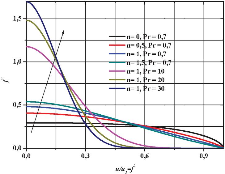
Figure 15 Variation of function $f^{\prime \prime }$ with $f^{\prime }$ for various values of n and Pr.

Variations of ${{\theta }^{\prime }|}_{\eta =0}$ as a function of $\eta$ for different Prandtl number values Pr derived from the FORTRAN calculation code are soon represented in Figure 16.

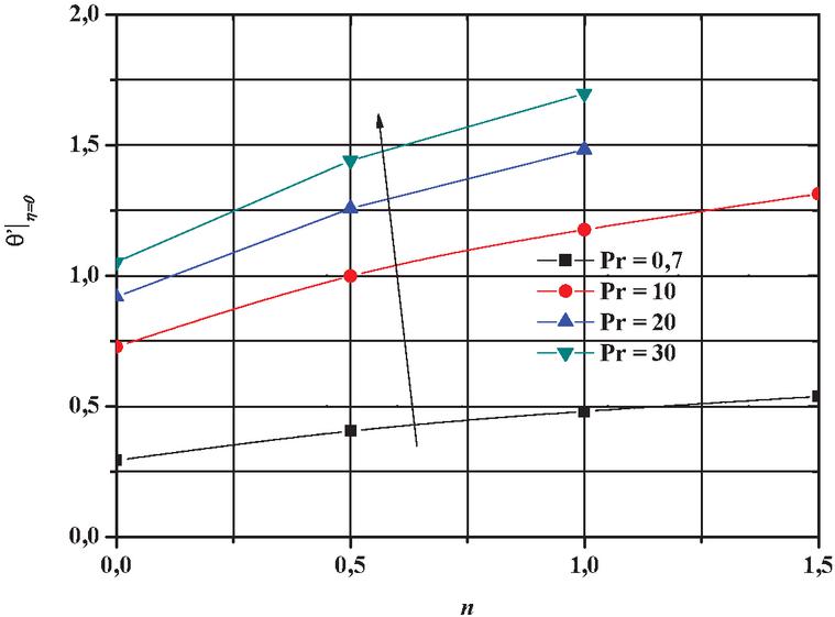
Figure 16 Variation of ${{\theta }^{\prime }|}_{\eta =0}$ as a function of n for different values of Pr.

For various values of the parameters that we have played on the simulation such as the number of exponents (n) and the number of Prandtl (Pr) in order to see their influence, temperature profiles are depicted in Figures 17–18 respectively.

According to the theory of boundary layer flow, the numerical results show that an increase in the Prandtl number results in a reduction in the thickness of the thermal boundary layer and, in general, a lower average temperature within the boundary layer. The logic is that low values of Pr are equivalent to increasing the thermal conductivity of the fluid, and therefore the heat is able to disperse away from the heating surface more quickly than for large values of. Pr. The Prandtl number controls the relative thickening of thermal boundary layers and momentum in thermal problems.

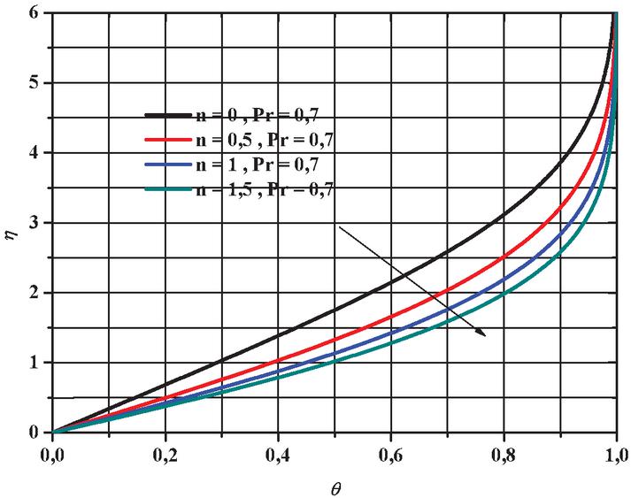
Figure 17 Effect of n on temperature profiles.

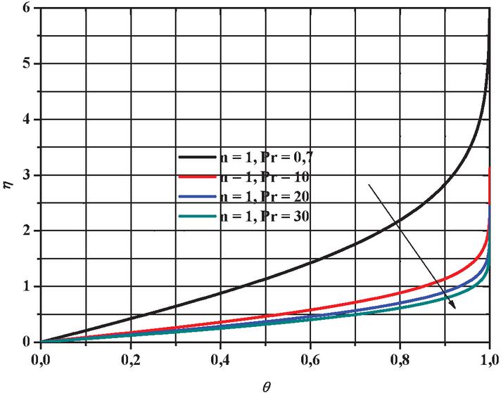
Figure 18 Effect of Pr on temperature profiles.

Figure 19 illustrates the simultaneous variation of dimensionless temperature profiles $\theta (\eta )$ with velocity field, both for different values of n and of Pr. We can see that the temperature field is rapidly increasing near the boundary layer by increasing the number of Prandtl. Physically speaking, the Prandtl number compares the speed of thermal phenomena and hydrodynamic phenomena in a fluid. A high Prandtl indicates that the temperature profile in the fluid will be strongly influenced by the velocity profile. A low Prandtl indicates that heat conduction is so fast that the velocity profile has little effect on the temperature profile.

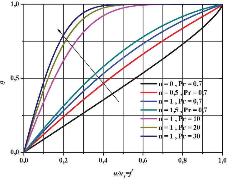
Figure 19 Plots of dimensionless temperature profiles for different Prandtl numbers and n (0, 0.5, 1, 1.5).

4.3 Computational Model Validation

In order to validate our numerical model which we performed on the flat plate, we carried out an in-depth search in the literature in which we came across several research works [1–11] which were similar to the one we treated, we have appropriately collected cases by case the numerical results from these investigations where we have been able to summarize them globally in Table 5.

Table 5 Comparison of the present results with published results [1–11] for $f^{\prime }(\eta )$

$\eta$	$df(\eta )/d\eta$ Present Work	$df(\eta )/d\eta$ Blasius [1]	$df(\eta )/d\eta$ Howarth [2]	$df(\eta )/d\eta$ Wan Zaimi et al. [3]	$df(\eta )/d\eta$ Ganji et al. [4]	$df(\eta )/d\eta$ Cortell [5]
0	0	0	0	0	0	0
1	0.328186	0.3298	0.32979	0.33	0.32978	0.32978
2	0.62755	0.6298	0.62977	0.63	0.62976	0.62977
3	0.844516	0.846	0.84605	0.848	0.84452	0.84605
4	0.954988	0.9555	0.95552	0.955	0.9028	0.95552
$\eta$	$df(\eta )/d\eta$ Yu and Chen [6]	$df(\eta )/d\eta$ Chang et al. [7]	$df(\eta )/d\eta$ Karabulut and Kiliç [8]	$df(\eta )/d\eta$ Majidian et al. [9]	$df(\eta )/d\eta$ Esmaeilpour and Ganji [10]	$df(\eta )/d\eta$ Fathizadeh and Rashidi [11]
0	0	0	0	0	0	0
1	0.32978	0.32979	0.3267	0.3300826	0.3462538	0.3494253
2	0.62977	0.62979	0.6241	0.6296405	0.6622097	0.6687189
3	0.84604	0.84608	0.8392	0.8455199	0.8854328	0.8947068
4	0.95552	0.95556	0.9489	0.960857	0.9762106	0.9826929

The third-order nonlinear differential Equation (37) with boundary conditions (38) was solved numerically using the fourth-order Runge-Kutta technique using FORTRAN programming. The numerical results of the present study are compared with published work by previous researchers and also are plotted in Figure 20. From this figure, we can see that the current results of this simulation are in good agreement with the exact solutions of Blasius [1] for the values $f^{\prime }(\eta )$, as well as for the previous numerical investigations of the other authors [2–11]. The numerical results show here, the efficiency of the procedure which we followed, and the precision of the proposed method for the resolution of the nonlinearity of the governing equation of the problem.

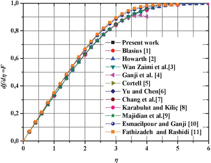
Figure 20 Numerical model validation and comparison of the velocity profiles with other research work.

In order to further strengthen the validation of our model, we also found other research in the literature that is related to the topic of scientific contribution. Thus, a comparison with other methods of solutions was entirely carried out namely; the Homotopy Perturbation Method (HPM) [9] described previously, differential transform method (DTM) [56], Laplace Transformation and New Homotopy Perturbation Method (LTNHPM) [57], Quartic B-Spline Method (QB-SM) [58], Power Technique of approximation series-Padé (PS-Padé) [59]. The results data of these investigations were collected from the literature and they are now summarized in Tables 6 and 7 with our numerical simulation results for approximation values of $f(\eta )$, and $f^{\prime }(\eta )$, respectively.

Table 6 Comparison of $f(\eta )$ between some numerical results and our results

	Present	HPM [9]	DTM [56]	LTNHPM	QB-SM [58]	PS-Pade
$\eta$	Work			[57]	h $=$ 0,01	[59]
0	0	0	0	0	0	0
0.4	0.02576	0.0265894	0.02656	0.02656	0.02656	0.026715
0.8	0.104247	0.1062224	0.10611	0.10611	0.10611	0.106727
1.2	0.234809	0.2381818	0.23795	0.23795	0.23795	0.239332
1.6	0.415768	0.4206587	0.42032	0.42032	0.42032	0.422749
2	0.644028	0.6503809	0.65002	0.65002	0.65002	0.653742
2.4	0.914934	0.9225139	0.92229	0.92228	0.92229	0.927492
2.8	1.222442	1.230937	1.23098	1.23098	1.23098	1.237797
3.2	1.559624	1.568863	1.56909	1.56909	1.56909	1.577606
3.6	1.919377	1.929627	1.92952	1.92952	1.92952	1.93975
4	2.295156	2.307278	2.30574	2.30575	2.30574	2.317668
4.4	2.681509	2.696739	2.69236	2.69242	2.69236	2.705933
4.8	3.07433	3.09348	3.08532	3.08718	3.08532	3.100462
5	3.272244	3.293258	3.28327	3.29272	3.28327

Table 7 Comparison of $f^{\prime }(\eta )$ between some numerical results and our results

$\eta$	Present Work	HPM [9]	DTM [56]	LTNHPM [57]	QB-SM [58] h $=$ 0,01
0	0	0	0	0	0
0.4	0.132073	0.1329106	0.13276	0.13276	0.13276
0.8	0.263387	0.2649775	0.26471	0.26471	0.26471
1.2	0.391951	0.3940826	0.39378	0.39378	0.39378
1.6	0.51462	0.5169439	0.51676	0.51676	0.51676
2	0.62755	0.6296405	0.62976	0.62977	0.62976
2.4	0.726917	0.7284483	0.72898	0.72898	0.72898
2.8	0.809775	0.8108053	0.81151	0.81151	0.81151
3.2	0.874771	0.8760235	0.87608	0.87608	0.87608
3.6	0.922444	0.9253044	0.92333	0.92333	0.92333
4	0.954988	0.960857	0.95552	0.95553	0.95552
4.4	0.975593	0.9845695	0.97587	0.97639	0.97587
4.8	0.987667	0.997382	0.98779	1.00322	0.98779
5	0.991467	0.9999982	0.99154	1.06671	0.99154

Figure 21 depicts the profile of function $f(\eta )$ for the different methods of solutions including that of ours. From this figure, we see that these methods from this figure, we see that these methods converge each of them, and the shapes of the curves are almost the same, and the gaits are almost the same. The results are found to be in good agreement. The results show that the method we performed is an efficient mathematical tool which can play a very important role in nonlinear science.

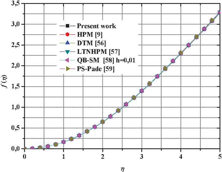
Figure 21 The comparison of $f(\eta )$ between our results and previous studies.

Figure 22 shows the variation of velocity profiles $(f^{\prime }(\eta ))$ with $\eta$. In this figure, the numerical results of our model are compared with the solution results of the research work that was performed previously. As we notice the bundles of curves are perfectly blended, there was good agreement between the present investigation and those of previous works.

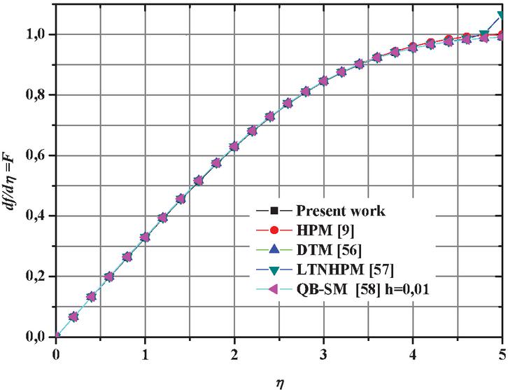
Figure 22 The comparison of $f^{\prime }(\eta )$ between our results and previous studies.

The solution method of the present work has been compared by the results of the analytical solution [8]. The value of the non-dimensional steam function $f(\eta )$ for various values of $\eta$, including the percentage of accuracy of the solution are all grouped together in Table 8.

Table 8 Comparison of calculated values of $f(\eta )$ with published analytical solution [8]

$\eta$	$f(\eta )$ Present Study	$f(\eta )$ Analytical Solution	Error %
0.000000	0.000000	0.0000	0.00
1.000000	0.163094	0.1556	4.59
2.000000	0.644028	0.6060	5.90
3.000000	1.387772	1.3518	2.59
4.000000	2.295155	2.2502	1.96
5.000000	3.272244	3.2117	1.85
6.000000	4.268533	4.1974	1.67

5 Conclusions

In this investigation, we have performed a numerical solution of the full Navier-Stokes and energy equations for flat plate flow in order to obtain heat transfer rates for situations involving external laminar flows. The thermal problem that we have treated of fluid over a flat plate aligned with the flow is a good model of situations that are of great practical importance. In order to easily solve these complex equations, the physical properties of the fluid were assumed to be constant and the flow was assumed two-dimensional as well as the dissipation effects in the global energy equation have been neglected, whose most of the solutions have been based on the use of the boundary layer equations.

Therefore, we have analyzed essentially two cases namely, one similarity solution for flow over an isothermal plate has a uniform surface temperature and another similarity solution for flow over a flat plate subjected to other thermal boundary conditions whose temperature varies with the spatial variable. Thus, we have resorted in this study to the exploitation of the similarity solution which uses as a starting point the assumption that the boundary layer profiles are similar to all the values of the spatial variable x. The governing equations describing the problem including the boundary conditions acting on the laminar boundary layer on the horizontal flat plate were reduced after the nondimensionalization phase of the solution of a set of nonlinear, coupled, partial differential equations for the unknown velocity and temperature field. The numerical solutions of the derivative equations were obtained using the fourth order Runge-Kutta method which were programmed under the Fortran language. The numerical results show a good agreement with the exact solution of Blasius equation and consistent with prior published results. The accuracy of the proposed method is higher than other approximation analytical solutions; hence suggests that the proposed method is efficient and practical. Several results have been discussed in depth according to their physical interpretations and important correlations have been relevantly drawn from this study, such as the velocity and temperature profile, the thermal boundary layer thickness, the heat transfer rate, the analytical expressions, local and mean Nusselt numbers.

The parameter involved in this study significantly affect the flow and heat transfer. The following conclusions can be drawn as a result of the computations:

• The temperature increases with increasing the Prandtl number.

• The Prandtl number is independent of the velocity profile in the flat plate boundary layer.

• The rate of heat transfer increases with increasing the Prandtl number.

• The increase of Prandtl number reduces the velocity along the plate

Finally, the numerical results of the model characterizing the behavior of the laminar boundary layer on a flat plate were validated and show that they were in good agreement with other previous investigations and they clearly reveal the effectiveness of the proposed approach. Mathematically, this analytic approach has general meanings and can be applied to solve many other non-similarity boundary-layer flows in fluid mechanics. The numerical results strongly display the efficiency and accuracy of the proposed method in solving the nonlinear equation.

Declaration of Conflict of Interest

The authors have declared no conflict of interest

References

[1] Blasius H. Grenzschichten in Flüssigkeiten mit kleiner Reibung. Z Math Phys, 1908, 56:1–37

[2] Howarth L. On the solution of the laminar boundary layer equations. Proc R Soc Lond Ser A, Math Phys Sci, 1938, 164:547–579

[3] Wan Mohd Khairy Adly Wan Zaimi, Biliana Bidin, Nor Ashikin Abu Bakar and Rohana Abdul Hamid, Applications of Runge-Kutta-Fehlberg Method and Shooting Technique for Solving Classical Blasius Equation, World Applied Sciences Journal 17, (Special Issue of Applied Math): 10–15, 2012

[4] Ganji, D.D., H. Babazadeh, F. Noori, M.M. Pirouz and M. Janipour. An Application of Homotopy Perturbation Method for Non-linear Blasius Equation to Boundary Layer Flow Over a Flat Plate. International Journal of Nonlinear Science, 2009, 7(4): 399–404.

[5] Cortell, R. Numerical solutions of the classical Blasius flat-plate problem. Applied Mathematics and Computation, 2005, vol. 170, pp. 706–710.

[6] Yu, L.-T., Chen, C.-K. The solution of the Blasius equation by the differential transformation method. Mathematical and Computer Modeling, 1998, vol. 28, pp. 101–111.

[7] Chih-Wen Chang, Jiang-RenChang and Chein-Shan Liu, The Lie-Group Shooting Method for Solving Classical Blasius Flat-Plate Problem, Computers, Materials & Continua CMC, vol. 7, no. 3, pp. 139–153, 2008.

[8] Utku Cem Karabulut, Alper Kiliç, Various techniques to solve Blasius equation, J. BAUN Inst. Sci. Technol., 20(3) Special Issue, 129–142, (2018).

[9] A. Majidian, M. khaki, M. khazayinejad, Analytical Solution of Laminar Boundary Layer Equations Over A Flat Plate by Homotopy Perturbation Method, International Journal of Applied Mathematical Research, 1(4) (2012) 581–592.

[10] Esmaeilpour, M. and D.D. Ganji. Application of He’s homotopy perturbation method to boundary layer flow and Convection heat transfer over a flat plate. Physics Letters A., 2007, 372(1): 33–38.

[11] M. Fathizadeh, F. Rashidi, Boundary layer convective heat transfer with pressure gradient using Homotopy Perturbation Method (HPM) over a flat plate, Chaos, Solitons and Fractals 42 (2009), pp. 2413–2419.

[12] Yang Zhou, Xiao-xue Hu, Ting Li, Dong-hai Zhang, Guo-qing Zhou, Similarity type of general solution for one-dimensional heat conduction in the cylindrical coordinate, International Journal of Heat and Mass Transfer 119 (2018) 542–550.

[13] Li-Wu Fan, Zi-Qin Zhu, Min-Jie Liu, A similarity solution to unidirectional solidification of nano-enhanced phase change materials (NePCM) considering the mushy region effect, International Journal of Heat and Mass Transfer 86 (2015) 478–481.

[14] Yutian Wang, Yiwen Li, Lianghua Xiao, Bailing Zhang, Yinghong Li, Similarity-solution-based improvement of $\gamma$-Re$\theta$t model for hypersonic transition prediction, International Journal of Heat and Mass Transfer 124 (2018) 491–503.

[15] S.K.S. Boetcher, E.M. Sparrow, Buoyancy-induced flow in an open-ended cavity: Assessment of a similarity solution and of numerical simulation model. International Journal of Heat and Mass Transfer 52(15–16) (2009), 3850–3856.

[16] Z.C. Wang, D.W. Tang, X.G. Hu, Similarity solutions for flows and heat transfer in microchannels between two parallel plates. International Journal of Heat and Mass Transfer 54(11–12) (2011), 2349–2354.

[17] V.R. Voller, A similarity solution for solidification of an under-cooled binary alloy, International Journal of Heat and Mass Transfer 49(11–12) (2006), 1981–1985.

[18] V.R. Voller, A similarity solution for the solidification of a multicomponent alloy, International Journal of Heat and Mass Transfer 40(12) (1997), 2869–2877.

[19] Shi-Jun Liao, Ioan Pop, Explicit analytic solution for similarity boundary layer equations, International Journal of Heat and Mass Transfer 47(1) (2004), 75–85.

[20] A. Yevtushenko, S. Koniechny, Similarity solutions of stationary thermoelasticity with the frictional heating, International Journal of Heat and Mass Transfer 42(18) (1999), 3539–3544.

[21] C.Y. Soong, G.J. Hwang, Effects of stress work on similarity solutions of mixed convection in rotating channels with wall-transpiration, International Journal of Heat and Mass Transfer 36(4) (1993), 845–856.

[22] J. Filipovic, R. Viskanta, F.P. Incropera, Similarity solution for laminar film boiling over a moving isothermal surface, International Journal of Heat and Mass Transfer 36(12) (1993), 2957–2963.

[23] Hsiao-Tsung Lin, Li-Kuo Lin, Similarity solutions for laminar forced convection heat transfer from wedges to fluids of any Prandtl number, International Journal of Heat and Mass Transfer 30(6) (1987), 1111–1118.

[24] Christine Doughty, Karsten Pruess, A similarity solution for two-phase fluid and heat flow near high-level nuclear waste packages emplaced in porous media, International Journal of Heat and Mass Transfer 33(6) (1990), 1205–1222.

[25] A.K. Kulkarni, H.R. Jacobs, J.J. Hwang, Similarity solution for natural convection flow over an isothermal vertical wall immersed in thermally stratified medium, International Journal of Heat and Mass Transfer 30(4) (1987), 691–698.

[26] Ming-Jer Huang, Cha’o-Kuang Chen, Local similarity solutions of free convective heat transfer from a vertical plate to non-Newtonian power law fluids, International Journal of Heat and Mass Transfer 33(1) (1990), 119–125.

[27] Asterios Pantokratoras, A note on natural convection along a convectively heated vertical plate, International Journal of Thermal Sciences 76 (2014), 221–224.

[28] Yang Zhou, Kang Wang, Similarity solution for one-dimensional heat equation in spherical coordinates and its applications, International Journal of Thermal Sciences 140 (2019), 308–318.

[29] Mohammad Mehdi Rashidi, NajibLaraqi, Seyed Majid Sadri, A novel analytical solution of mixed convection about an inclined flat plate embedded in a porous medium using the DTM-Padé, International Journal of Thermal Sciences 49(12) (2010), 2405–2412.

[30] De-Yi Shang, Liang-Cai Zhong, A similarity transformation of velocity field and its application for an in-depth study on laminar free convection heat transfer of gases, International Journal of Thermal Sciences, 101 (2016), 106–115.

[31] B. Weigand, A. Birkefeld, Similarity solutions of the entropy transport, International Journal of Thermal Sciences, 48(10) (2009), 1863–1869.

[32] Shwin-Chung, Wong Shih-Han, Chu Ming-Hsuan Ai, Revisit on natural convection from vertical isothermal plate arrays II—3-D plume buoyancy effects, International Journal of Thermal Sciences, 126 (2018), 205–217.

[33] Shwin-Chung, Wong Shih-Han, Chu, Revisit on natural convection from vertical isothermal plate arrays–effects of extra plume buoyancy, International Journal of Thermal Sciences, 120 (2017), 263–272.

[34] Asterios Pantokratoras, Natural convection along a vertical isothermal plate with linear and non-linear Rosseland thermal radiation, International Journal of Thermal Sciences, 84 (2014), 151–157.

[35] R. Muthucumaraswamy, P. Ganesan, V.M. Soundalgekar, On flow and heat transfer of a viscous incompressible fluid past an impulsively started vertical isothermal plate, International Journal of Thermal Sciences, 40(3) (2001), 297–302.

[36] R.J. Goldstein, U. Madanan, T.H. Kuehn, Simplified correlations for free convection from a horizontal isothermal cylinder, Applied Thermal Engineering, 161 (2019), 113832.

[37] David H. Schultz, Robert T. Balmer, Similarity solutions for the converging or diverging steady flow of non-newtonian elastic power law fluids with wall suction or injection—II Axisymmetric conical flow, Computers & Fluids, 6(4) (1978), 271–284.

[38] Yulin Wu, Shuhong Liu, Hua-Shu Dou, Shangfeng Wu, Tiejun Chen, Numerical prediction and similarity study of pressure fluctuation in a prototype Kaplan turbine and the model turbine, Computers & Fluids, 56(15) (2012), 128–142.

[39] Harry A. Dwyera, J. Grcarb, Solution of the Navier–Stokes equation with finite-differences on unstructured triangular meshes, Computers & Fluids, 27(5–6) (1998), 695–708.

[40] Natalia C. Roşcaioan Pop, Unsteady boundary layer flow of a nanofluid past a moving surface in an external uniform free stream using Buongiorno’s model, Computers & Fluids, 95(22) (2014), 49–55.

[41] Norfifah Bachok, Mihaela Anghel Jaradat and Ioan Pop, A similarity solution for the flow and heat transfer over a moving permeable flat plate in a parallel free stream. Heat and Mass Transfer, 47 (2011), 1643.

[42] J. R. Fan, J. M. Shi and X. Z. Xu, Similarity solution of mixed convection over a horizontal moving plate, Heat and Mass Transfer, 32 (1997), 199–206.

[43] J. Fan, J. Shi and X. Xu, Similarity solution of free convective boundary-layer behavior at a stretching surface, Heat and Mass Transfer, 35 (1999), 191–196.

[44] M. A. Chaudhary, J. H. Merkin and I. Pop, Similarity solutions in free convection boundary-layer flows adjacent to vertical permeable surfaces in porous media: II prescribed surface heat flux, Heat and Mass Transfer, 30 (1995), 341–347.

[45] Ali Al-Mudhaf and Ali J. Chamkha, Similarity solutions for MHD thermosolutal Marangoni convection over a flat surface in the presence of heat generation or absorption effects, Heat and Mass Transfer, 42 (2005), 112–121.

[46] A. A. Mohammadein, Similarity analysis of axisymmetric free convection on a horizontal infinite plate subject to a mixed thermal boundary condition in a micropolar fluid, Heat and Mass Transfer, 36 (2000), 209–212.

[47] Ali J. Chamkha and Abdul-Rahim A. Khaled, Similarity solutions for hydromagnetic simultaneous heat and mass transfer by natural convection from an inclined plate with internal heat generation or absorption, Heat and Mass Transfer, 37 (2001), 117–123.

[48] Tiegang Fang, Similarity solution of thermal boundary layers for laminar narrow axisymmetric jets, International Journal of Heat and Fluid Flow, 23 (2002), 840–843.

[49] D. Ewing, Two-point similarity in turbulent planar jet flows, International Journal of Heat and Fluid Flow, 67(Part B) (2017), 131–138.

[50] T. Yilmaz, Numerical solution of Navier-stokes equations for laminar fluid flow in rows of plates in staggered arrangement, International Journal of Heat and Fluid Flow, 3(4) (1982), 201–206.

[51] Gabriclla Bognär, Similarity solution of boundary layer flows for non-Newtonian fluids, International Journal of Nonlinear Sciences & Numerical Simulation, 10(11–12) (2009), 1555–1566.

[52] Ali Belhocine and Wan Zaidi Wan Omar. An analytical method for solving exact solutions of the convective heat transfer in fully developed laminar flow through a circular tube, Heat Transfer Asian Research, 46(8) (2017), 1342–1353.

[53] Ali Belhocine and Wan Zaidi Wan Omar. Numerical study of heat convective mass transfer in a fully developed laminar flow with constant wall temperature, Case Studies in Thermal Engineering, 6 (2015), 43–60.

[54] Ali Belhocine and Oday Ibraheem Abdullah, Numerical simulation of thermally developing turbulent flow through a cylindrical tube, Int. J. Adv. Manuf. Technol. 102(5–8) (2019), 2001–2012.

[55] Ali Belhocine and Wan Zaidi Wan Omar. Analytical solution and and numerical simulation of the generalized Levèque equation to predict the thermal boundary layer, Mathematics and Computers in Simulation. 180 (2021), 43–60.

[56] H Aminikhah, Analytical Approximation to the Solution of Nonlinear Blasius’ Viscous Flow Equation by LTNHPM, ISRN Mathematical Analysis 2012, pp. 1–10.

[57] H. Aminikhah and S. Kazemi? Numerical Solution of the Blasius Viscous Flow Problem by Quartic B-Spline Method, International Journal of Engineering Mathematics, 2016, 1–6.

[58] S. A. Lal and N. M. Paul, “An accurate taylors series solution with high radius of convergence for the Blasius function and parameters of asymptotic variation,” Journal of Applied Fluid Mechanics, vol. 7, no. 4, pp. 557–564, 2014.

[59] A. Noghrehabadi, M. Ghalambaz and A. Samimi, Approximate solution of laminar thermal boundary layer over a thin plate heated from below by convection, Journal of Computational and Applied Research in Mechanical Engineering, 2(2) (2013), 45–57.

Biographies

Ali Belhocine received his Magister degree in Mechanical Engineering in 2006 from Mascara University, Mascara, Algeria. After then, he was a PhD student at the University of Science and the Technology of Oran (USTO Oran), Algeria. He has recently obtained his Ph.D. degrees in Mechanical Engineering at the same University. His research interests include Automotive Braking Systems, Finite Element Method (FEM), ANSYS simulation, CFD Analysis, Heat Transfer, Thermal-Structural Analysis, Tribology and Contact Mechanic.

Nadica Stojanovic, Bachelor, Master degree obtained at the University of Kragujevac, Faculty of Engineering. Scientific fields – Motor vehicles and motors. Her research areas cover FE analysis, thermal-mechanical analysis, aerodynamics, ergonomics, and environmental science. Workplace – Assistant at the University of Kragujevac, Faculty of engineering. She participates in the project “Research on vehicle safety as part of the cybernetic system: driver – vehicle – environment” of the Ministry of Education, Science and Technological Development of the Republic of Serbia. Authorized by the Traffic Safety Agency for testing and control of imported vehicles and modified vehicles.

Oday Ibraheem Abdullah has obtained his M.Sc degree in Mechanical Eng./University of Baghdad in 2003. He is one of the faculty members in the Department of Energy Engineering/College of Engineering/University of Baghdad since 2002. Now he is a research associate in the System Technology and Mechanical Design Methodology/Hamburg University of Technology. His research interests cover Automobile Engineering, Automotive Industry, Design Engineering, CAD Design Optimization, Finite Element Analysis, Stress Analysis and Tribology.

European Journal of Computational Mechanics, Vol. 30_4–6, 337–386.
doi: 10.13052/ejcm2642-2085.30463
© 2021 River Publishers