Numerical Analysis of a SUSHI Scheme for an Elliptic-parabolic System Modeling Miscible Fluid Flows in Porous Media

Mohamed Mandari, Mohamed Rhoudaf and Ouafa Soualhi

Moulay Ismail University, Meknes, Morocco

E-mail: mandariart@gmail.com; rhoudafmohamed@gmail.com; ouafasoualhi@gmail.com

Received 28 March 2019; Accepted 12 November 2019; Publication 14 January 2020

Abstract

In this paper, we demonstrate the convergence of a schema using stabilization and hybrid interfaces applying to partial differential equations describing miscible displacement in porous media. This system is made of two coupled equations: an anisotropic diffusion equation on the pressure and a convection-diffusion-dispersion equation on the concentration of invading fluid. The anisotropic diffusion operators in both equations require special care while discretizing by a finite volume method SUSHI. Later, we present some numerical experiments.

Keywords: Porous media, nonconforming grids, finite volume schemes, SUSHI, convergence analysis.

1 Introduction

The single-phase miscible displacement of one fluid by another in a porous medium is modeling by a system of nonlinear partial differential equations. In the literature, there exists several modelling approaches, in [2–6] the authors are introduced the Peaceman model where the fluids are considered incompressible this model is constituted of an elliptic parabolic coupled system. While, if the fluids are compressible, the system becomes parabolic see [7] and [8]. We are interested in the study of The first model, it is constituted of an anisotropic diffusion equation on the pressure and a convection-diffusion-dispersion equation on the concentration of the invading fluid, see [9] for the theoretical analysis of this system of partial differential equations.

The miscible displacement problem studied in this work consists of a nonlinear elliptic-parabolic coupled system, it has been the subject of several studies, C. Chainais-Hillairet, S. Krell and A. Mouton, in [10] and [11], are study the numerical analysis and the convergence of a schema DDFV, on the other hand in [12] Chainais-Hillairet and Droniou were proposed the scheme of mixed finite volume, Hanzhang Hu, Yiping Fu and Jie Zhou study this model by the mixed finite elements in [13]. The authors in [14, 15] studied the Finite Element schemes for both equations. We refer to [27,28] for the Eulerian-Lagrangian localized adjoint method combined with the mixed finite element methods. See [16] for the convergence analysis for a discontinuous Galerkin finite element. Then, he pressure equation was dis-cretised by finite element method and the concentration equation by method of characteristics in [17–19], let cite other references that study the miscible displacement problems by different methods [24–26].

The unknowns of the problem are p the pressure in the mixture, U its Darcy velocity and c the concentration of the invading fluid. The porous medium is characterized by its porosity ϕ(x) and its permeability A(x). We denote by μ(c) the viscosity of the fluid mixture, $\widehat{c}$ the injected concentration, q⁺ and q⁻ are the injection and the production source terms. The model on a time interval (0, T) and a domain Ω ⊂ ℝ² is defined by the following system

$$\{\begin{array}{ll}\text{div}(U)=q^{+}-q^{-}\hfill & \text{in }(0,T)\times \Omega ,\hfill \\ U=-K(x,c)\nabla p\hfill & \text{in }(0,T)\times \Omega ,\hfill \\ {\displaystyle {\int }_{\Omega }}p(.,x)\mathit{dx}=0\hfill & \text{On }(0,T),\hfill \end{array}$$

(1)

$$\varphi (x){\partial }_{t}c-\text{div}(D(x,U)\nabla c)+\text{div}(Uc)+q^{-}c=\widehat{c}{q}^{+}\text{ in }(0,T)\times \Omega .$$

(2)

Where

• The domain Ω is an open, bounded, connected subset of ℝ^d (d = 2 or d = 3). Which supported tube polygonal (d = 2) or polyhedral (d = 3), and ∂Ω stands for its boundary.
• The initial condition is given by

  $$c(x,0)=c_0(x),$$

  (3)

  
  such that

  $$c_0\in L^{\infty }(\Omega ),\text{ and satisfies }0\le c_0\le 1\text{ a}\text{.e}\text{. in }\Omega ,$$

  (4)

• The Neumann boundary conditions are defined by

  $$\{\begin{array}{ll}U.n=0\hfill & \text{on }]0,T[\times \partial \Omega ,\hfill \\ D(x,U)\nabla c.n=0\hfill & \text{on }]0,T[\times \partial \Omega .\hfill \end{array}$$

  (5)

• The porous medium is characterized by the porosity ϕ(x) with

  $$\varphi \in L^{\infty }(\Omega )\text{ and there exists }{\varphi }^{*}>0\text{ such that}:{\varphi }_{*}\le \varphi \le {\varphi }_{*}^{-1}\text{ a}\text{.e}\text{. in }\Omega .$$

  (6)

• $K(x,c)=\frac{A(x)}{\mu (c)}$ and D are the diffusion-dispersion tensors including molecular diffusion and mechanical dispersion, verified the following properties:

  $$\{\begin{array}{l}K:\Omega \times ℝ\to M_2(ℝ)\text{ is a Caratheodory matrix-valued function satisfying:}\hfill \\ \exists {\alpha }_K>0\text{ s}\text{.t}\text{. }K(x,s)\xi .\xi \ge {\alpha }_K|\xi {|}^2\text{for a}\text{.e}\text{. }x\in \Omega ,\text{ all }s\in ℝ,\text{ and all }\xi \in {ℝ}^2,\hfill \\ \exists {\Lambda }_K>0\text{ s}\text{.t}\text{.}|K(x,s)|\le {\Lambda }_K\text{ for a}\text{.e}\text{. }x\in \Omega \text{ and all }s\in ℝ,\hfill \end{array}$$

  (7)

  
  and

  $$\{\begin{array}{l}D:\Omega \times {ℝ}^2\to M_2(ℝ)\text{ is a Caratheodory matrix-valued function satisfying:}\hfill \\ \exists {\alpha }_D>0\text{ s}\text{.t}\text{. }D(x,V)\xi .\xi \ge {\alpha }_D(1+|V|)|\xi {|}^2\text{for a}\text{.e}\text{. }x\in \Omega ,\text{ all }(V,\xi )\in {ℝ}^2\times {ℝ}^2,\hfill \\ \exists {\Lambda }_D>0\text{ s}\text{.t}\text{.}|D(x,V)|\le {\Lambda }_D(1+|V|)\text{ for a}\text{.e}\text{. }x\in \Omega \text{ and all }V\in {ℝ}^2,\hfill \end{array}$$

  (8)

• D is given by

  $$D(x,U)=\varphi (x)(d_{m}I+|U|(d_{l}E(U)+d_t(I-E(U)))),$$

  (9)

  
  I is the identity matrix, d_m is the molecular diffusion, d_l and d_t are the longitudinal and transverse dispersion coefficients, and $E(U)={(\frac{U_i{U}_j}{|U{|}^2})}_{1\le i,j\le d}$.
• We denote by μ(c) the viscosity of the fluid mixture as

  $$\mu (c)=\mu (0){\left(1+(M^{\frac{1}{4}}-1)c\right)}^{-4}\text{on }[0,1],$$

  (10)

  
  $M=\frac{\mu (0)}{\mu (1)}$ is the mobility ratio (we extend μ to ℝ by letting μ = μ(0) on] − ∞, 0[and μ = μ(1) on ]1, ∞[).
• $\widehat{c}$ is the injected concentration such that

  $$\widehat{c}\in L^{\infty }(]0,T[\times \Omega )\text{ satisfies}:0\le \widehat{c}\le 1\text{ a}\text{.e}\text{. in }]0,T[\times \Omega .$$

  (11)

• q⁺ and q⁻ are the injection and the production source terms

  $$\{\begin{array}{l}(q^{+},q^{-})\in L^{\infty }(0,T;L^2(\Omega ))\text{ are non negative functions such that }(\text{s}\text{.t}\text{.}),\hfill \\ {\displaystyle {\int }_{\Omega }}{q}^{+}(.,x)\mathit{dx}={\displaystyle {\int }_{\Omega }}{q}^{-}(.,x)\mathit{dx}\text{ almost everywhere }(\text{a}\text{.e}\text{.})\text{ on }]0,T[.\hfill \end{array}$$

  (12)

Definition 1.1 (Weak solution) Under the hypotheses (3–12). A weak solution of (1) and (2) is a triple of functions $(\overline{p},\overline{U},\overline{c})$ satisfying: $(\overline{p}\in L^{\infty }(0,T;H^1(\Omega )))$, (Ū ∈ L^∞(0,T; L²(Ω))) and $(\widehat{c}\in L^{\infty }(0,T;L^2(\Omega ))\cap L^2(0,T;H^1(\Omega )))$

$$\{\begin{array}{ll}{\displaystyle {\int }_{\Omega }}\overline{p}(t,.)\mathit{dt}=0\mathit{for\; all\; a.e\; t}\in ]0,T[,\hfill & \overline{U}=K(x,\overline{c})\nabla \overline{p}\mathit{in}]0,T[\times \Omega ,\hfill \\ a_1(\overline{p},{\phi }_1)={\displaystyle {\int }_0^T}{\displaystyle {\int }_{\Omega }}{q}^{+}{\phi }_1+{\displaystyle {\int }_0^T}{\displaystyle {\int }_{\Omega }}{q}^{-}{\phi }_1\hfill & \forall {\phi }_1\in C^{\infty }([0,T]\times \overline{\Omega }),\hfill \\ a_2(\overline{c},{\phi }_2)={\displaystyle {\int }_0^T}{\displaystyle {\int }_{\Omega }}\widehat{c}{q}^{+}{\phi }_2\hfill & \forall {\phi }_2\in C_c^{\infty }([0,T]\times \overline{\Omega }),\hfill \end{array}$$

(13)

with

$$\{\begin{array}{l}{a}_1(\overline{p},{\phi }_1)={\displaystyle {\int }_0^T}{\displaystyle {\int }_{\Omega }}K(x,c)\nabla \overline{p}\nabla {\phi }_1,\hfill \\ a_2(\overline{c},{\phi }_2)=-{\displaystyle {\int }_0^T}{\displaystyle {\int }_{\Omega }}\varphi (x)\overline{c}{\partial }_t{\phi }_2+{\displaystyle {\int }_0^T}{\displaystyle {\int }_{\Omega }}D(x,\overline{U})\nabla \overline{c}\nabla {\phi }_2\hfill \\ -{\displaystyle {\int }_0^T}{\displaystyle {\int }_{\Omega }}\overline{c}\overline{U}\nabla {\phi }_2+{\displaystyle {\int }_0^T}{\displaystyle {\int }_{\Omega }}{q}^{+}\overline{c}{\phi }_2-{\displaystyle {\int }_{\Omega }}\phi c_0(x){\phi }_2(0,.),\hfill \end{array}$$

(14)

In this work, we want to apply one of the finite volume methods dedicated to anisotropic diffusion. We will examine the application of a finite volume scheme using stabilization and hybrid interfaces, which has been proposed by Eymard et al. [20], to the diffusion term in the pressure equation and in the concentration convection-diffusion-dispersion equation of the system describing miscible fluid flows in porous media (Peaceman model). This method is characterized by:

• Using a single mesh that is very general, unstructured and does not take into account the condition of orthogonality (Finite Volume method [29]).
• Avoid to project the gradient on the edges of dual and primal mesh (method DDFV [30]) by the addition of a term of stability which stabilize the gradient obtained by the method of the finite volume 4, so, the number of variables of SUSHI method is less compared to the method (DDFV).

We present and study a numerical scheme and convergence analysis for SUSHI method applying to this model, more precisely. In order to prove the convergence of the SUSHI schemes, we apply a similar strategy as [8] on our numerical approximation instead of the regularization of the Peaceman model. Then, Some numerical tests are also carried out to verify the validity of the numerical scheme proposed.

This article is organized as follows. In Section 2 we present meshes and the associated notations, than, we introduce the different discrete operators (gradient, diffusion and convection operators) and some proprieties. The main result of the paper is detailed in Section 3 as follows Sections 3.1, 3.2 and 3.3 are devoted for the discretization of the system (1–12), in Section 3.4 we present some numerical experiments. Finally we demonstrate the convergence theorem in Section 3.5.

2 The Finite Volume Scheme SUSHI

The SUSHI scheme is based on two schemes, firstly the Hybrid Finite Volume (HVF) scheme introduced in 2007 by R. Eymard et al. [23]. This HVF scheme, adapted to solve the anisotropic diffusion problem, introduces additional unknowns on the edges of the meshes in order to reconstruct the discrete gradient in all directions and thus to correctly treat the anisotropic and heterogeneous problems, and secondly on the cell-centered SUCCES scheme (Finite volume method classic).

The originality of this scheme (HVF) lies in the proof of convergence that only requires weak hypotheses on the mesh. This HVF scheme was then modified and gave birth to the SUSHI schemes in 2009 [20].

There are two variants of the SUSHI schema: a first one where the unknowns on the edges are only introduced where they are needed, for example where there are strong heterogeneities and a second where the unknowns on the edges are introduced on all the edges of the mesh.

In this section, we will present different definitions, notations and conventions of writing that we will use later, on the other hand, we follow the idea of Eymard et al. [20] to build flux using a stabilized discrete gradient. After, we define the discretization of the convection term, then, we give some proprieties and definition of the SUSHI schemes.

2.1 Space and Time Discretization

Definition 2.1 Let’s define some notations of the discretization of Ω.

• A discretization of Ω is defined by 𝒟 = (ℳ, ℰ, P).
• ℳ is a family of connected non-empty open subspaces included in Ω (set of control volumes 𝒦).
• σ is a non-empty open of ℝ.
• ℰ is the set of the interfaces σ.
• ℰ is decomposed into two subdomains ℰ_int and ℰ_ext which are respectively the sets of interfaces inside and outside to the mesh 𝒟.
• For all 𝒦 ∈ ℳ, M_σ = {𝒦, σ ∈ ℰ_𝒦}.
• x_σ and x_𝒦 are respectively the center and the barycentre of σ and 𝒦.
• m_𝒦 and m_σ are respectively the measure of control volume 𝒦 and of interface σ.
• n_𝒦,σ is the unit vector normal to σ outward to 𝒦.
• P is the set of points of Ω.
• C_𝒦,σ is the cone with vertex x_𝒦 and basis σ.

Definition 2.2 We consider X_𝒟, X_𝒟,0 and X_𝒟,0,ℬ three spaces defined as follow:

$$X_{𝒟}=\{\upsilon =({({\upsilon }_{𝒦})}_{𝒦\in ℳ},{({\upsilon }_{\sigma })}_{\sigma \in ℰ});{\upsilon }_{𝒦}\in ℝ,{\upsilon }_{\sigma }\in ℝ\},$$

(15)

$$X_{𝒟,0}=\{\upsilon \in X_{𝒟}\mathit{such\; that}{\Lambda }_{𝒦}{\nabla }_{𝒦,\sigma }^n\upsilon .n_{𝒦,\sigma }=0,\forall \sigma \in {ℰ}_{\mathit{ext}}\},$$

(16)

$$X_{𝒟,0,ℬ}=\left\{\upsilon \in X_{𝒟,0}/\exists {\beta }_{\sigma }^{𝒦}\in ℝ;{\upsilon }_{\sigma }={\displaystyle \sum _{𝒦\in ℳ}}{\beta }_{\sigma }^{𝒦}{\upsilon }_{𝒦}\right\}.$$

(17)

With ℬ is defined in the next definition.

Definition 2.3 Let:

$$u_{\sigma }={\displaystyle \sum _{𝒦\in ℳ}}{\beta }_{\sigma }^{𝒦}{u}_{𝒦},$$

(18)

where ${({\beta }_{\sigma }^{𝒦})}_{𝒦\in ℳ,\sigma \in {ℰ}_{\mathit{int}}}$ is a family of real numbers, with ${\beta }_{\sigma }^{𝒦}\ne 0$ only for some control volumes 𝒦, close to σ, and such that

$${\displaystyle \sum _{𝒦\in ℳ}}{\beta }_{\sigma }^{𝒦}=1\mathit{and}{x}_{\sigma }={\displaystyle \sum _{𝒦\in ℳ}}{\beta }_{\sigma }^{𝒦}{x}_{𝒦}.$$

(19)

ℬ is the set of the eliminated unknowns using (18), and ℋ = ℰ_int/ℬ.

The projections in the spaces X_𝒟, X_𝒟,0 and X_𝒟,0,ℬ are defined in the definition next.

Definition 2.4 $C_0(\overline{\Omega })$ is the set of continues functions which are null in ∂Ω. for all $\psi \in C_0(\overline{\Omega })$, we define

1. The projection in X_𝒟 by $$\begin{array}{l}{𝒫}_{𝒟}:C_0(\overline{ℝ})\to X_{𝒟}\hfill \\ \psi \mapsto {𝒫}_{𝒟}\psi =({(\psi (x_{𝒦}))}_{𝒦\in M},{(\psi (x_{\sigma }))}_{\sigma \in ℰ}).\hfill \end{array}$$
2. 𝒫_𝒟,ℬψ = v is an element of X_𝒟,ℬ such that v_𝒦 = ψ(x_𝒦), ∀𝒦, ∈ ℳ; v_σ = v_𝒦, for all σ ∈ ℰ_ext; v_σ = ψ(x_σ), for all σ ∈ ℋ and ${\upsilon }_{\sigma }={\displaystyle {\sum }_{𝒦\in ℳ}}{\beta }_{\sigma }^{𝒦}\psi (x_{𝒦})$ for all σ ∈ ℬ.
3. 𝒫_ℳ ∈ H_ℳ(Ω) (H_ℳ(Ω) is the set of the piece-wise function in central volume 𝒦 ∈ ℳ) such that 𝒫_ℳ(ψ(x)) = ψ(x_𝒦), a.s ∀_x ∈ 𝒦, ∀𝒦 ∈ ℳ.

The space X_𝒟 is equipped with the semi-norm |.|_X𝒟 defined by

$$|\upsilon {|}_{X_{𝒟}}^2={\displaystyle \sum _{𝒦\in ℳ}}{\displaystyle \sum _{\sigma \in {ℰ}_{𝒦}}}\frac{m_{\sigma }}{d_{𝒦\sigma }}{({\upsilon }_{\sigma }-{\upsilon }_{𝒦})}^2,\text{ for all }\upsilon \in X_{𝒟}.$$

(20)

Note that |.|_X𝒟 is a norm on the spaces X_𝒟,0 and X_𝒟,0,ℬ.

Definition 2.5 The time interval (0, T) (T > 0) is divided to N (N is an integer such that N > 0) small intervals have a step δt equals to T/N, where δt = t_n+1 − t_n we introduce this spaces

$$X_{𝒟,\delta t}=\{{({\upsilon }^n)}_{n\in \{0,\mathrm{...},N-1\}},{\upsilon }^n\in X_{𝒟}\},$$

(21)

$$X_{𝒟,\delta t,0}=\{{({\upsilon }^n)}_{n\in \{0,\mathrm{...},N-1\}},{\upsilon }^n\in X_{𝒟,0}\},$$

(22)

$$X_{𝒟,\delta t,ℬ}=\{{({\upsilon }^n)}_{n\in \{0,\mathrm{...},N-1\}},{\upsilon }^n\in X_{𝒟,0,ℬ}\}.$$

(23)

The semi-norm on X_𝒟,δt is defined by

$$|\upsilon {|}_{X_{𝒟,\delta t}}^2={\displaystyle \sum _{n=0}^{N-1}}\delta t|{\upsilon }^n{|}_{X_{𝒟}}^2.$$

(24)

2.2 The Discrete Gradient

It is always possible to deduce an expression for ∇_𝒟u(x) as a linear combination of (u_σ − u_𝒦)_σ∈ℰ𝒦. Let us first define

$$\begin{array}{l}{\nabla }_{𝒦}:X_{𝒟}\to H_{ℳ}{(\Omega )}^d\hfill \\ u^{n+1}\mapsto {\nabla }_{𝒦}{u}^{n+1},\hfill \end{array}$$

such that

$$u^{n+1}\in X_D,{\nabla }_{𝒦}{u}^{n+1}=\frac{1}{|𝒦|}{\displaystyle \sum _{\sigma \in {ℰ}_{𝒦}}}|\sigma |[u_{\sigma }^{n+1}-u_{𝒦}^{n+1}]n_{𝒦,\sigma }.$$

However, we find that this discrete gradient is zero for any $u_{𝒦}^{n+1}\in 𝒦$, if $u_{\sigma }^{n+1}$ are zero, so it is not coercive. We thus seek a new coherent discrete gradient with the previous and coercive in the C_𝒦,σ (cone the vertex x_𝒦 and basis σ). This corresponds to the previous step gradient to which we add a correction term. We define the discrete gradient as follows:

$${\nabla }_{𝒦,\sigma }{u}^{n+1}={\nabla }_{𝒦}{u}^{n+1}+{ℛ}_{𝒦,\sigma }(u^{n+1})n_{𝒦,\sigma },$$

(25)

with

$${ℛ}_{𝒦,\sigma }(u^{n+1})=\frac{\sqrt{d}}{d_{𝒦,\sigma }}(u_{\sigma }^{n+1}-u_{𝒦}^{n+1}-{\nabla }_{𝒦}{u}^{n+1}.[x_{\sigma }-x_{𝒦}]).$$

(Recall that d is the space dimension and d_𝒦,σ is the Euclidean distance between x_𝒦 and x_σ) We obtain the following stable discrete gradient

$${\nabla }_{𝒦,\sigma }{u}^{n+1}={\nabla }_{𝒦}{u}^{n+1}+{ℛ}_{𝒦,\sigma }{u}^{n+1}.n_{𝒦,\sigma },$$

(26)

We may then define ∇_𝒟 as the piece-wise constant function equal to ∇_𝒦,σ a.e. in the cone C_𝒦,σ with vertex x_𝒦 and basis σ

$${\nabla }_{𝒟}{u}^{n+1}={\nabla }_{𝒦,\sigma }{u}^{n+1}\text{ for a}\text{.e }x\in C_{𝒦,\sigma }.$$

(27)

Then we have

$${\nabla }_{𝒦,\sigma }{u}^{n+1}={\displaystyle \sum _{{\sigma }^{\prime }{ℰ}_{𝒦}}}{Y}^{\sigma ,{\sigma }^{\prime }}(u_{{\sigma }^{\prime }}^{n+1}-u_{𝒦}^{n+1}),$$

(28)

with Y^σ,σ′ giving by

$$Y^{\sigma ,{\sigma }^{\prime }}=\{\begin{array}{ll}\frac{m_{\sigma }}{m_{𝒦}}{n}_{𝒦\sigma }+\frac{\sqrt{d}}{d_{𝒦,\sigma }}(1-\frac{m_{\sigma }}{m_{𝒦}}{n}_{𝒦\sigma }.[x_{\sigma }-x_{𝒦}])n_{𝒦\sigma }\hfill & \text{if }\sigma ={\sigma }^{\prime },\hfill \\ \frac{m_{{\sigma }^{\prime }}}{m_{𝒦}}{n}_{𝒦{\sigma }^{\prime }}-\frac{\sqrt{d}}{d_{𝒦,\sigma }{m}_{𝒦}}{n}_{𝒦,{\sigma }^{\prime }}.[x_{\sigma }-x_{𝒦}]n_{𝒦,\sigma }\hfill & \text{otherwise}\text{.}\hfill \end{array}$$

(29)

2.3 The Discrete Convection Term

To treat the convection term in the concentration equation, we define the following convection operator discrete:

$$\begin{array}{l}{\mathit{divc}}_{\sigma }:{ℝ}^{𝒟}\times {ℝ}^{𝒟}\to {ℝ}^{𝒟}\hfill \\ ({\xi }_{𝒟},{\upsilon }_{𝒟})\mapsto \mathit{div}({\xi }_{𝒟},{\upsilon }_{𝒟}),\hfill \end{array}$$

with

$${\mathit{divc}}_{\sigma }({\xi }_{𝒟},{\upsilon }_{𝒟})=\{\begin{array}{ll}{\upsilon }_{𝒦}{n}_{\sigma ,𝒦}{\xi }_{𝒦}\hfill & \text{if }{\upsilon }_{𝒦}{n}_{\sigma ,𝒦}\ge 0,\hfill \\ -{\upsilon }_{𝒦}{n}_{\sigma ,𝒦}{\xi }_{𝒦}\hfill & \text{if }{\upsilon }_{𝒦}{n}_{\sigma ,𝒦}<0.\hfill \end{array}$$

(30)

2.4 The Proprieties of the Schemes

Let 𝒟 be a discretisation of Ω in the sense of Definition (2.1). The size of the discretisation 𝒟 is defined by

$$h_{𝒟}=\underset{𝒦\in ℳ}{{\displaystyle \sup }}(d(𝒦)),$$

(31)

with d(𝒦) is the diameter of 𝒦 and the regularity of the mesh is defined by

$${\theta }_{𝒟}=\max \left(\underset{\sigma 𝒦,ℒ\in {ℰ}_{\mathit{int}}}{{\displaystyle \max }}\left(\frac{d_{𝒦,\sigma }}{d_{ℒ,\sigma }}\right),\underset{𝒦\in ℳ,\sigma \in {ℰ}_{𝒦}}{{\displaystyle \max }}\left(\frac{d(𝒦)}{d_{𝒦,\sigma }}\right)\right)\text{}.$$

(32)

For a given set ℬ ∈ ℰ_int and for a given family ${\beta }_{\sigma }^{𝒦}$ satisfying property (18), we introduce a measure of the resulting regularity by

$${\theta }_{𝒟,ℬ}=\max \left({\theta }_{𝒟},\underset{𝒦\in ℳ,\sigma \in ℰ\cap ℬ}{{\displaystyle \max }}\frac{{\displaystyle \sum _{ℒ\in ℳ}}|{\beta }_{\sigma }^{ℒ}||x_{ℒ}-x_{\sigma }{|}^2}{h_{𝒟}^2}\right)\text{}.$$

(33)

Definition 2.6 Let 𝒟 be a discretisation of Ω in the sense of Definition (2.1), and let δt be the time step defined in Definition (2.5). For v ∈ X_𝒟, we define the following related norm

$${\Vert P_{ℳ}\upsilon \Vert }_{1,2,ℳ}^2={\displaystyle \sum _{𝒦\in ℳ}}{\displaystyle \sum _{\sigma \in ℰ}}|\sigma |d_{𝒦,\sigma }{\left(\frac{{𝒟}_{\sigma }\upsilon }{d_{\sigma }}\right)}^2,$$

(34)

and for v ∈ X_𝒟,δt, we define the following related norm

$${\Vert {𝒫}_{ℳ}\upsilon \Vert }_{1;1,2,ℳ}^2={\displaystyle \sum _{n=0}^{N-1}}\delta t{\Vert {𝒫}_{ℳ}{\upsilon }^n\Vert }_{1,2,ℳ}^2,$$

(35)

with d_σ = |d_𝒦,σ + d_ℒ,σ|, D_σv = |v_𝒦 − v_ℒ| if ℳ_σ = {𝒦, ℒ}, and d_σ = d_𝒦,σ, D_σv = |v_𝒦| if ℳ_σ = {𝒦}.

A result stated in [20] gives the relation

$${\Vert {𝒫}_{ℳ}\upsilon \Vert }_{1,2,ℳ}^2\le |\upsilon {|}_{X_{𝒟}}^2,\forall \upsilon \in X_{𝒟,0}.$$

(36)

Then, we get

$${\Vert {𝒫}_{ℳ}\upsilon \Vert }_{1;1,2,ℳ}^2\le |\upsilon {|}_{X_{𝒟},\delta t}^2,\forall \upsilon \in X_{\delta t,𝒟,0}.$$

(37)

A result stated in [20] gives the relation

$${\Vert {𝒫}_{ℳ}\upsilon \Vert }_{1,2,ℳ}^2\le |\upsilon {|}_{X_{𝒟}}^2,\forall \upsilon \in X_{𝒟,0}.$$

(38)

Then, we get

$${\Vert {𝒫}_{ℳ}\upsilon \Vert }_{1;1,2,ℳ}^2\le |\upsilon {|}_{X_{𝒟},\delta t}^2,\forall \upsilon \in X_{\delta t,𝒟,0}.$$

(39)

We recall in this section some proprieties of SUSHI scheme. The proof of these proprieties can be found in [21].

Lemma 2.7 Let 𝒟 be a discretisation of Ω in the sense of Definition (2.1). Let ν > 0 be such that $\nu \le \frac{d_{𝒦,\sigma }}{d_{ℒ,\sigma }}\le \frac{1}{\nu }$ for all σ ∈ ℰ, where M_σ = |𝒦, ℒ}. Then there exists C₁ only depending on d, Ω and ν such that

$${\Vert {𝒫}_{ℳ}\upsilon \Vert }_{{ℒ}^2(\Omega )}\le C_1{\Vert {𝒫}_{ℳ}\upsilon \Vert }_{1,2,ℳ},\forall \upsilon \in X_{𝒟},$$

(40)

where ‖𝒫_ℳv‖_1,2,ℳ is defined by (34).

Lemma 2.8 Let 𝒟 be a discretisation of Ω in the sense of Definition (2.1), and let δt be the time step defined in Definition (2.5). Let ν > 0 be such that $\nu \le \frac{d_{𝒦,\sigma }}{d_{ℒ,\sigma }}\le \frac{1}{\nu }$ for all σ ∈ ℰ, where M_σ = {𝒦, ℒ}. Then there exists $C_1^{\prime }$ only depending on δt and C₁ such that

$${\Vert {𝒫}_{ℳ}\upsilon \Vert }_{L^2(0,T;L^2(\Omega ))}\le C_1^{\prime }{\Vert {𝒫}_{ℳ}\upsilon \Vert }_{1;1,2,ℳ},\forall \upsilon \in X_{𝒟,\delta t},$$

(41)

where ‖𝒫_ℳv‖_1;1,2,ℳ is defined by (35).

Proof 2.9 The proof is a result of Lemma 2.7.

Definition 2.10 Let 𝒟 be a discretisation of Ω in the sense of the Definition (2.1), and δt be a time step defined in Definition (2.5). We define the L² − norm of the discrete gradient by

$${\Vert {\nabla }_{𝒟}\upsilon (x)\Vert }_{L^2{(\Omega )}^d}^2={\displaystyle \sum _{K\in ℳ}}{\displaystyle \sum _{\sigma \in {ℰ}_K}}\frac{\left|\sigma \right|d_{K,\sigma }}{d}|{\nabla }_{K,\sigma }\upsilon {|}^2,\forall \upsilon \in X_{𝒟},$$

and

$$\begin{array}{r}\hfill {\Vert {\nabla }_{𝒟}w(x,t)\Vert }_{L^2(0,T;L^2{(\Omega )}^d)}^2={\displaystyle \sum _{n=1}^N}\delta t{\displaystyle \sum _{K\in ℳ}}{\displaystyle \sum _{\sigma \in {ℰ}_K}}\frac{\left|\sigma \right|d_{K,\sigma }}{d}|{\nabla }_{K,\sigma }{w}^n{|}^2,\\ \hfill \forall w\in X_{𝒟,\delta t},\end{array}$$

where ∇_𝒦,σ and ∇_𝒟 is defined by (26) and (27)

Lemma 2.11 Let 𝒟 be a discretisation of Ω in the sense of the Definition (2.1), and δt be a time step defined in Definition (2.5) and we assume that there exists a positive θ such that θ_𝒟 ≤ θ for all 𝒟,

1. Then there exist positive constants C₂ and C₃ only depending on θ and d such that

   $$C_2|\upsilon {|}_{X_{𝒟}}^2\le |\left|{\nabla }_{𝒟}\upsilon \right|{|}_{L^2{(\Omega )}^d}^2\le C_3|\upsilon {|}_{X_{𝒟}}^2\forall \upsilon \in X_{𝒟}.$$

   (42)

2. Moreover, we have

   $$C_4|w{|}_{X_{𝒟,\delta t}}^2\le |\left|{\nabla }_{𝒟}w\right|{|}_{L^2(0,T;L^2{(\Omega )}^d}^2\le C_5|w{|}_{X_{𝒟,\delta t}}^2\forall \upsilon \in X_{𝒟\delta t}.$$

   (43)

Definition 2.12 Let 𝒟 be a discretisation of Ω in the sense of Definition (2.1) and δt be a time step defined in Definition (2.5). Let u_𝒟,δt ∈ X_𝒟,δt be a solution of the problem. Then, 𝒫^ℳu_𝒟,δt(x, t) is an approximate solution of the problem.

Lemma 2.13 (Discrete gradient consistency) Let 𝒟 be a discretisation of Ω in the sense of Definition 2.1, and θ ≥ θ_𝒟 given. Then, for any function $\psi \in C^2(\overline{\Omega })$, there exists C₆ only depending on d, θ and ψ such that

$${\Vert {\nabla }_{𝒟}{𝒫}_{𝒟}\psi -\nabla \psi \Vert }_{{(L^{\infty }(\Omega ))}^d}\le C_6{h}_{𝒟},$$

(44)

where ∇_𝒟 is defined by (25–27).

Lemma 2.14 (A compactness lemma) Let Ω be a bounded open subset of ℝ^d, T > 0 and $A\subset L^1(0,T;L_{\mathit{Loc}}^1(\Omega ))$. If A is relatively compact in $L^1(0,T;(C_c^2(\Omega ){)}^{\prime })$ and for all ω relatively compact in Ω,

$$\underset{u\in A}{{\displaystyle \sup }}{\Vert u(.,.+\xi )-u\Vert }_{L^1(]0,T[\times \omega )}\to 0\mathit{as}\left|\xi \right|\to 0.$$

Then, A is relatively compact in $L^1(0,T;L_{\mathit{Loc}}^1(\Omega ))$.

Proof 2.15 The proof of this propriety can be found in [12].

2.5 Discrete Weak Formulation

In this section we present the discrete weak formulation for the problem (1–2). We consider, for all n = 0, ..., N − 1 and all 𝒦 ∈ ℳ, unknowns cⁿ⁺¹ ∈ X_𝒟,δt, Uⁿ ∈ X_𝒟,δt and pⁿ ∈ X_𝒟,δt which stand for approximate values of c, U and p on [n; n + 1],

2.5.1 Equation of the pressure

We begin with the discretisation of this equation

$$-\text{div}(K(x,c)\nabla p)=q^{+}-q^{-}.$$

(45)

We integer over 𝒦 for any 𝒦 ∈ ℳ and in the interval ]tⁿ, tⁿ⁺¹[⊂]0,T[ that which yields

$${\displaystyle {\int }_K}{\displaystyle {\int }_{t^n}^{t^{n+1}}}-\mathit{div}(K(x,c)\nabla p)={\displaystyle {\int }_K}{\displaystyle {\int }_{t^n}^{t^{n+1}}}(q^{+}-q^{-}),$$

that’s gives

$$\delta t{\displaystyle {\int }_{𝒦}}-\text{div}(K(x,c^n)\nabla p^{n+1})=\delta t{\displaystyle {\int }_{𝒦}}(q^{+,n+1}-q^{-,n+1}),$$

then

$${\displaystyle \sum _{\sigma \in {ℰ}_{𝒦}}}{\displaystyle {\int }_{\sigma }}K(x,c^n)\nabla p^{n+1}.n_{𝒦,\sigma }=m_{𝒦}(q_{𝒦}^{+,n+1}-q_{𝒦}^{-,n+1}),$$

finally

$${\displaystyle \sum _{\sigma \in {ℰ}_{𝒦}}}{ℱ}_{𝒦,\sigma }^1(p^{n+1})=m_{𝒦}{q}_{𝒦}^{+,n+1}-𝒦q_{𝒦}^{-,n+1}.$$

(46)

For the border elements, we obtain the equations by discretising the second part of the system (5), then we have

$$K(x,c_{𝒦}^n){\nabla }_{𝒦,\sigma }{p}^{n+1}.n_{𝒦,\sigma }=0,\forall \sigma \in {ℰ}_{\mathit{ext}}.$$

(47)

We use the fact that the flow is continuous at the interface of the two elements, we have then

$$F_{𝒦,\sigma }^1(p^{n+1})+F_{ℒ,\sigma }^1(p^{n+1})=0\text{ for all }\sigma \in {ℰ}_{\mathit{int}}\text{ such that }{ℳ}_{\sigma }=\{𝒦,ℒ\}.$$

(48)

And now we have card(ℰ_int) + card(ℰ_ext) + card(ℳ) unknowns and equations.

Let, multiplying the equation (46) by ${\upsilon }_{𝒦}^{n+1}$ for all 𝒦 ∈ ℳ and all n = 0, ..., N − 1, then sum over 𝒦 and over n = 0, ..., N − 1, we get

$${\displaystyle \sum _{n=0}^{N-1}}{\displaystyle \sum _{𝒦\in ℳ}}{\displaystyle \sum _{\sigma \in {ℰ}_{𝒦}}}{ℱ}_{𝒦}^1(p^{n+1}){\upsilon }_{𝒦}^{n+1}={\displaystyle \sum _{n=0}^{N-1}}{\displaystyle \sum _{𝒦\in ℳ}}{\upsilon }_{𝒦}^{n+1}{m}_{𝒦}(q_{𝒦}^{+,n+1}-q_{𝒦}^{-,n+1}),$$

(49)

which gives

$$<p,\upsilon {>}_{F^1}={\displaystyle \sum _{n=0}^{N-1}}{\displaystyle \sum _{𝒦\in ℳ}}{\upsilon }_{𝒦}^{n+1}{m}_{𝒦}(q_{𝒦}^{+,n+1}-q_{𝒦}^{-,n+1}),$$

(50)

with

$$<p,\upsilon {>}_{F^1}={\displaystyle \sum _{n=0}^{N-1}}{\displaystyle \sum _{𝒦\in ℳ}}{\displaystyle \sum _{\sigma \in {ℰ}_{𝒦}}}{F}_{𝒦}^1(p^{n+1})[{\upsilon }_{𝒦}^{n+1}-{\upsilon }_{\sigma }^{n+1}].$$

(51)

We define also

$${[p^{n+1},{\upsilon }^{n+1}]}_{F^1}={\displaystyle \sum _{𝒦\in ℳ}}{\displaystyle \sum _{\sigma \in {ℰ}_{𝒦}}}{F}_{𝒦}^1(p^{n+1})[{\upsilon }_{𝒦}^{n+1}-{\upsilon }_{\sigma }^{n+1}].$$

(52)

2.5.2 The constitutive law of the model adopted

For the second equation we have

$$U=-K(x,c)\nabla p,\text{ in }]0,T[\times \Omega .$$

(53)

We integer over 𝒟 such that 𝒟 ∈ 𝔇 with 𝔇 is the set of diamond Ω, and over the time interval ]tⁿ, tⁿ⁺¹ [⊂]0, T[, we obtain

$${\displaystyle {\int }_{t^n}^{t^{n+1}}}{\displaystyle {\int }_{𝒟}}\mathit{Udxdt}={\displaystyle {\int }_{t^n}^{t^{n+1}}}{\displaystyle {\int }_{𝒟}}-𝒦(x,c)\nabla \mathit{pdxdt},$$

(54)

after simplifications we obtain the following formula

$$U_{𝒟}^{n+1}={(-𝒦(x_{\sigma },c^n)\nabla p^{n+1})}_{𝒟}.$$

Since for any diamond 𝒟 ∈ 𝔇, we have

$$𝒟=\{\begin{array}{ll}\{𝒦,\sigma \}\cup \{ℒ,\sigma \}\hfill & \text{if }\sigma \in {ℰ}_{\mathit{int}},\hfill \\ \{𝒦,\sigma \}\hfill & \text{if }\sigma \in {ℰ}_{\mathit{extt}}.\hfill \end{array}$$

Then

$$U_{𝒟}^{n+1}=\{\begin{array}{ll}{U}_{𝒦,\sigma }^{n+1}+U_{ℒ,\sigma }^{n+1},\hfill & \text{if }\sigma \in {ℰ}_{\mathit{int}},\hfill \\ U_{𝒦,\sigma }^{n+1},\hfill & \text{if }\sigma \in {ℰ}_{\mathit{ext}},\hfill \end{array}$$

and

$${\nabla }^{𝒟}{p}^{n+1}=\{\begin{array}{cc}{\nabla }_{𝒦,\sigma }{p}^{n+1}+{\nabla }_{ℒ,\sigma }{p}^{n+1},& \text{if }\sigma \in {ℰ}_{\mathit{int}}\\ {\nabla }_{𝒦,\sigma }{p}^{n+1},& \text{if }\sigma \in {ℰ}_{\mathit{ext}}.\end{array}$$

Finally, we get

$$\{\begin{array}{ll}{U}_{𝒦,\sigma }^{n+1}+U_{ℒ,\sigma }^{n+1}=-𝒦(x_{\sigma },c_{𝒦}^n){\nabla }_{𝒦,\sigma }{p}^{n+1}-𝒦(x_{\sigma },c_{ℒ}^n){\nabla }_{ℒ,\sigma }{p}^{n+1},\hfill & \text{if }\sigma \in {ℰ}_{\mathit{int}},\hfill \\ U_{𝒦,\sigma }^{n+1}=-K(x_{\sigma },c_{𝒦}^n){\nabla }_{𝒦,\sigma }{p}^{n+1},\hfill & \text{if }\sigma \in {ℰ}_{\mathit{ext}},\hfill \end{array}$$

(55)

with ∇_𝒟,σpⁿ⁺¹, ∇_ℒ,σpⁿ⁺¹ are noted in (28).

(55) write in other way by

$$\{\begin{array}{ll}{U}_{𝒦,\sigma }^{n+1}.n_{\sigma ,𝒦}+U_{ℒ,\sigma }^{n+1}.n_{\sigma ,ℒ}={ℱ}_{𝒦,\sigma }^1(p^{n+1})+{ℱ}_{ℒ,\sigma }^1(p^{n+1}),\hfill & \text{if}\sigma \in {ℰ}_{\mathit{int}}\hfill \\ U_{𝒦,\sigma }^{n+1}.n_{\sigma ,𝒦}=F_{𝒦,\sigma }^1(p^{n+1}),\hfill & \text{otherwise}\text{.}\hfill \end{array}$$

(56)

2.5.3 Concentration equation

Now, use discrete the following third equation

$$\varphi (x){\partial }_{t}c-\mathit{div}(D(x,U)\nabla c)+\mathit{div}(cU)+q^{-}c=q^{+}\widehat{c}.$$

(57)

We integrate over the volume control 𝒦 ∈ ℳ and over the time interval ]tⁿ, tⁿ⁺¹[⊂ [0,T] we obtain

$$\begin{array}{l}{\displaystyle {\int }_{t^n}^{t^{n+1}}}{\displaystyle {\int }_{𝒦}}\varphi (x){\partial }_{t}c-{\displaystyle {\int }_{t^n}^{t^{n+1}}}{\displaystyle {\int }_{𝒦}}\mathit{div}(D(x,U)\nabla c)\hfill \\ +{\displaystyle {\int }_{t^n}^{t^{n+1}}}{\displaystyle {\int }_{𝒦}}\mathit{div}(cU)+{\displaystyle {\int }_{t^n}^{t^{n+1}}}{\displaystyle {\int }_{𝒦}}{q}^{-}c={\displaystyle {\int }_{t^n}^{t^{n+1}}}{\displaystyle {\int }_{𝒦}}{q}^{+}\widehat{c}.\hfill \end{array}$$

Then

$$\begin{array}{l}{\displaystyle {\int }_{𝒦}}\varphi (x)(c^{n+1}-c^n)-\delta t\text{}\text{}{\displaystyle {\int }_{𝒦}}\mathit{div}(D(x,U^{n+1})\nabla c^{n+1})+\delta t\text{}\text{}{\displaystyle {\int }_{𝒦}}\mathit{div}(c^{n+1}{U}^{n+1})\hfill \\ +\delta t{\displaystyle {\int }_{𝒦}}{q}^{-,n+1}{c}^{n+1}=\delta t{\displaystyle {\int }_{𝒦}}{q}^{+,n+1}{\widehat{c}}^{n+1},\hfill \end{array}$$

we get

$$\begin{array}{l}{m}_{𝒦}{\varphi }_{𝒦}(c_{𝒦}^{n+1}-c_{𝒦}^n)+\delta t{\displaystyle \sum _{\sigma \in {ℰ}_{𝒦}}}{F}_{𝒦,\sigma }^2(c^{n+1})+\delta t{\displaystyle \sum _{\sigma \in {ℰ}_{𝒦}}}{m}_{\sigma }{\mathit{divc}}_{\sigma }(c_{𝒟}^{n+1},U_{𝒟}^{n+1})\hfill \\ +\delta {\mathit{tm}}_{𝒦}{q}_{𝒦}^{-,n+1}{c}_{𝒦}^{n+1}=\delta {\mathit{tm}}_{𝒦}{q}_{𝒦}^{+,n+1}{\widehat{c}}_{𝒦}^{n+1}.\hfill \end{array}$$

(58)

We have card(ℳ) equations and card(ℰ) + card(ℳ) unknowns, for a reasonable system we need to card(ℰ) equations, for that we have

$$𝒟(x_{𝒦},U_{𝒦}^{n+1}){\nabla }_{𝒦,\sigma }{c}^{n+1}.n_{𝒦,\sigma }=0,\forall \sigma \in {ℰ}_{\mathit{ext}},$$

(59)

and since the flux is continuous with the interface of the two elements, then we have

$$F_{𝒦,\sigma }^2(c^{n+1})+F_{ℒ,\sigma }^2(c^{n+1})=0\text{ for all }\sigma \in {ℰ}_{\mathit{int}}\text{ such that }{ℳ}_{\sigma }=\{𝒦,ℒ\}.$$

(60)

We have now card(ℰ_int) + card(ℰ_ext) + card(ℳ) unknowns and equations.

We multiplying (58) by $w_{𝒦}^{n+1}$ for all w_𝒦 ∈ ℳ and all n = 0, ..., N − 1, then sum over 𝒦 and over n = 0, ..., N − 1, then we get

$$\begin{array}{l}{\displaystyle \sum _{n=0}^{N-1}}{\displaystyle \sum _{𝒦\in ℳ}}{w}_{𝒦}^{n+1}{\varphi }_{𝒦}(c_{𝒦}^{n+1}-c_{𝒦}^n)+\delta t{\displaystyle \sum _{n=0}^{N-1}}{\displaystyle \sum _{𝒦\in ℳ}}{\displaystyle \sum _{\sigma \in {ℰ}_{𝒦}}}{ℱ}_{𝒦,\sigma }^2(c^{n+1})w_{𝒦}^{n+1}\hfill \\ +\delta t{\displaystyle \sum _{n=0}^{N-1}}{\displaystyle \sum _{𝒦\in ℳ}}{w}_{𝒦}^{n+1}{\displaystyle \sum _{\sigma \in {ℰ}_{𝒦}}}{m}_{\sigma }{\mathit{divc}}_{\sigma }(c_{𝒟}^{n+1},U_{𝒟}^{n+1})\hfill \\ +\delta t{\displaystyle \sum _{n=0}^{N-1}}{\displaystyle \sum _{𝒦\in ℳ}}{w}_{𝒦}^{n+1}{q}_{𝒦}^{-,n+1}{c}_{𝒦}^{n+1}=\delta t{\displaystyle \sum _{n=0}^{N-1}}{\displaystyle \sum _{𝒦\in ℳ}}{w}_{𝒦}^{n+1}{q}_{𝒦}^{+,n+1}{\widehat{c}}_{𝒦}^{n+1}.\hfill \end{array}$$

Bearing in mind (60), from above, we get

$$\begin{array}{l}{\displaystyle \sum _{n=0}^{N-1}}{\displaystyle \sum _{𝒦\in ℳ}}{w}_{𝒦}{\varphi }_{𝒦}(c_{𝒦}^{n+1})-\delta t{\displaystyle \sum _{n=0}^{N-1}}{\displaystyle \sum _{𝒦\in ℳ}}{\displaystyle \sum _{\sigma \in {ℰ}_{𝒦}}}{ℱ}_{𝒦,\sigma }^2(c^{n+1})[w_{𝒦}^{n+1}-w_{\sigma }^{n+1}]\hfill \\ +\delta t{\displaystyle \sum _{n=0}^{N-1}}{\displaystyle \sum _{𝒦\in ℳ}}{w}_{𝒦}^{n+1}{\displaystyle \sum _{\sigma \in {ℰ}_{𝒦}}}{m}_{\sigma }{\mathit{divc}}_{\sigma }(c_{𝒟}^{n+1},U_{𝒟}^{n+1})\hfill \\ +\delta t{\displaystyle \sum _{n=0}^{N-1}}{\displaystyle \sum _{𝒦\in ℳ}}{w}_{𝒦}^{n+1}{q}_{𝒦}^{-,n+1}{c}_{𝒦}^{n+1}\hfill \\ =\delta t{\displaystyle \sum _{n=0}^{N-1}}{\displaystyle \sum _{𝒦\in ℳ}}{w}_{𝒦}^{n+1}[q_{𝒦}^{+,n+1}{\widehat{c}}_{𝒦}^{n+1}+{\varphi }_{𝒦}(c_{𝒦}^n)],\hfill \end{array}$$

thus, we give as a form of bilinear approximation the following formula

$$\{\begin{array}{l}<c,w{>}_{F^2}={\displaystyle \sum _{n=0}^{N-1}}{\displaystyle \sum _{𝒦\in ℳ}}\text{}{w}_{𝒦}^{n+1}{\varphi }_{𝒦}(c_{𝒦}^{n+1})+\delta t{\displaystyle \sum _{n=0}^{N-1}}{\displaystyle \sum _{𝒦\in ℳ}}{\displaystyle \sum _{\sigma \in {ℰ}_{𝒦}}}{ℱ}_{𝒦,\sigma }^2(c^{n+1})[w_{𝒦}^{n+1}-w_{\sigma }^{n+1}]\hfill \\ +\delta t{\displaystyle \sum _{n=0}^{N-1}}{\displaystyle \sum _{𝒦\in ℳ}}{w}_{𝒦}^{n+1}{\displaystyle \sum _{\sigma \in {ℰ}_{𝒦}}}{m}_{\sigma }{\mathit{divc}}_{\sigma }(c_{𝒟}^{n+1},U_{𝒟}^{n+1})+\delta t{\displaystyle \sum _{n=0}^{N-1}}{\displaystyle \sum _{𝒦\in ℳ}}{w}_{𝒦}^{n+1}{q}_{𝒦}^{-,n+1}{c}_{𝒦}^{n+1}.\hfill \end{array}$$

(61)

We define also

$$\{\begin{array}{l}{[c^{n+1},w^{n+1}]}_{F^2}={\displaystyle \sum _{𝒦\in ℳ}}\frac{w_{𝒦}^{n+1}{\varphi }_{𝒦}}{\delta t}(c_{𝒦}^{n+1})+{\displaystyle \sum _{𝒦\in ℳ}}{\displaystyle \sum _{\sigma \in {ℰ}_{𝒦}}}{ℱ}_{𝒦,\sigma }^2(c^{n+1})[w_{𝒦}^{n+1}-w_{\sigma }^{n+1}]\hfill \\ +{\displaystyle \sum _{𝒦\in ℳ}}{w}_{𝒦}^{n+1}{\displaystyle \sum _{\sigma \in {ℰ}_{𝒦}}}{m}_{\sigma }{\mathit{divc}}_{\sigma }(c_{𝒟}^{n+1},U_{𝒟}^{n+1})+{\displaystyle \sum _{𝒦\in ℳ}}{w}_{𝒦}^{n+1}{q}_{𝒦}^{-,n+1}{c}_{𝒦}^{n+1}.\hfill \end{array}$$

(62)

2.6 The Discrete Flux

The discrete flux ${ℱ}_{𝒦,\sigma }^1$ and ${ℱ}_{𝒦,\sigma }^2$ are expressed in terms of the discrete unknowns. For this purpose we apply the SUSHI scheme proposed in [20]. The idea is based upon the identification of the numerical flux through the mesh dependent bilinear form, using the expression of the discrete gradient

$$\begin{array}{l}{\displaystyle \sum _{n=0}^{N-1}}{\displaystyle \sum _{𝒦\in ℳ}}{\displaystyle \sum _{\sigma \in {ℰ}_{𝒦}}}{ℱ}_{𝒦,\sigma }^1(p^{n+1})(u_{𝒦}-u_{\sigma })\hfill \\ \approx {\displaystyle {\int }_0^T}{\displaystyle {\int }_{\Omega }}{\nabla }_{𝒟}{p}^{n+1}K(x,s){\nabla }_{𝒟}u,\forall p^{n+1},u\in X_{0,𝒟},\hfill \end{array}$$

(63)

and

$$\begin{array}{l}{\displaystyle \sum _{n=0}^{N-1}}{\displaystyle \sum _{𝒦\in ℳ}}{\displaystyle \sum _{\sigma \in {ℰ}_{𝒦}}}{ℱ}_{𝒦,\sigma }^2(c^{n+1})({\upsilon }_{𝒦}-{\upsilon }_{\sigma })\hfill \\ \approx {\displaystyle {\int }_0^T}{\displaystyle {\int }_{\Omega }}{\nabla }_{𝒟}{c}^{n+1}D(x,U^{n+1}){\nabla }_{𝒟}\upsilon ,\forall c^{n+1},\upsilon \in X_{0,𝒟}.\hfill \end{array}$$

(64)

The identification of the numerical fluxes using relation (63) and (64) leads to the expression

$$F_{𝒦,\sigma }^1(p^n)={\displaystyle \sum _{{\sigma }^{\prime }\in {ℰ}_{𝒦}}}{𝒦}_{𝒦}^{\sigma ,{\sigma }^{\prime }}(p_{𝒦}^{n+1}-p_{\sigma }^{n+1}),$$

(65)

$$F_{𝒦,\sigma }^2(c^{n+1})={\displaystyle \sum _{{\sigma }^{\prime }\in {ℰ}_{𝒦}}}{D}_{𝒦}^{\sigma ,{\sigma }^{\prime }}(c_{𝒦}^{n+1}-c_{\sigma }^{n+1}).$$

(66)

Thus

$${\displaystyle {\int }_{𝒦}}{\nabla }_{𝒟}{p}^{n+1}K(x,c^n){\nabla }_{𝒟}u={\displaystyle \sum _{\sigma \in {ℰ}_{𝒦}}}{\displaystyle \sum _{{\sigma }^{\prime }\in {ℰ}_{𝒦}}}{K}_{𝒦}^{\sigma ,{\sigma }^{\prime }}(p_{𝒦}^{n+1}-p_{{\sigma }^{\prime }}^{n+1})(u_{{\sigma }^{\prime }}-u_{𝒦}).$$

(67)

$${\displaystyle {\int }_{𝒦}}{\nabla }_{𝒟}{c}^{n+1}D(x,U^{n+1}){\nabla }_{𝒟}v={\displaystyle \sum _{\sigma \in {ℰ}_{𝒦}}}{\displaystyle \sum _{{\sigma }^{\prime }\in {ℰ}_{𝒦}}}{D}_{𝒦}^{\sigma ,{\sigma }^{\prime }}(c_{𝒦}^{n+1}-c_{{\sigma }^{\prime }}^{n+1})(v_{{\sigma }^{\prime }}-v_{𝒦}).$$

(68)

With σ, σ′ ∈ ℰ_𝒦 and

$$\{\begin{array}{ll}{K}_{𝒦}^{\sigma ,{\sigma }^{\prime }}={\displaystyle \sum _{{\sigma }^{″}\in {ℰ}_{𝒦}}}{Y}^{{\sigma }^{″},\sigma }{\Gamma }_{𝒦}^{{\sigma }^{″}}{Y}^{{\sigma }^{″},{\sigma }^{\prime }}\hfill & \text{with }{\Gamma }_{𝒦}^{{\sigma }^{″}}={\displaystyle {\int }_{𝒦,C_{{\sigma }^{″}}}}K(x,c^n)\mathit{dx},\hfill \\ D_{𝒦}^{\sigma ,{\sigma }^{\prime }}={\displaystyle \sum _{{\sigma }^{″}\in {ℰ}_{𝒦}}}{Y}^{{\sigma }^{″},\sigma }{\Theta }_{𝒦}^{{\sigma }^{″}}{Y}^{{\sigma }^{″},{\sigma }^{\prime }}\hfill & \text{with }{\Theta }_{𝒦}^{{\sigma }^{″}}={\displaystyle {\int }_{𝒦,C_{{\sigma }^{″}}}}D(x,U^{n+1})\mathit{dx}.\hfill \end{array}$$

The local matrices $K_{𝒦}^{\sigma ,{\sigma }^{\prime }}$ and $D_{𝒦}^{\sigma ,{\sigma }^{\prime }}$ are symmetric and positive.

2.7 Final Scheme

Using (26) we have

$$\{\begin{array}{l}{\nabla }_{𝒦,\sigma }{p}^{n+1}={\nabla }_{𝒦}{p}^{n+1}+{ℛ}_{𝒦,\sigma }{p}^{n+1}.n_{𝒦,\sigma },\hfill \\ {\nabla }_{𝒦,\sigma }{c}^{n+1}={\nabla }_{𝒦}{c}^{n+1}+{ℛ}_{𝒦,\sigma }{c}^{n+1}.n_{𝒦,\sigma },\hfill \end{array}$$

and

$${\mathit{divc}}_{\sigma }({\xi }_{𝒟},v_{𝒟})=\{\begin{array}{ll}{v}_{𝒦}{n}_{\sigma ,𝒦}{\xi }_{𝒦}\hfill & \text{if }{v}_{𝒦}{n}_{\sigma ,𝒦}\ge 0,\hfill \\ -v_{𝒦}{n}_{\sigma ,𝒦}{\xi }_{ℒ}\hfill & \text{if }{v}_{𝒦}{n}_{\sigma ,𝒦}<0.\hfill \end{array}$$

The discretisation of the problems (1) and (2) is defined as following:

$$c(x,0)=\frac{1}{m_{𝒦}}{\displaystyle {\int }_{𝒦\in ℳ}}{c}_0(x)\mathit{dx}.$$

(69)

$${\displaystyle \sum _{𝒦\in ℳ}}{m}_{𝒦}{p}_{𝒦}=0.$$

(70)

$$\{\begin{array}{l}{D}_{𝒦,\sigma }{\nabla }_{𝒟}c.n=0\hfill \\ U_{𝒟}.n=0.\hfill \end{array}$$

(71)

$$\{\begin{array}{l}\text{Find for all }𝒦\in ℳ\text{ and for all instant }n,p^{n+1}\text{ and }{c}^{n+1}\hfill \\ {\displaystyle \sum _{\sigma \in {ℰ}_{𝒦}}}{\displaystyle \sum _{{\sigma }^{\prime }\in {ℰ}_{𝒦}}}{A}_{𝒦}^{\sigma {\sigma }^{\prime }}[p_{\sigma }^{n+1}-p_{𝒦}^{n+1}][v_{{\sigma }^{\prime }}-v_{𝒦}]=m_{𝒦}{v}_{𝒦}(q_{𝒦}^{+,n+1}-q_{𝒦}^{-,n+1}),\hfill \\ U_{𝒟}^{n+1}=K(x,c_{𝒦}^n)){\nabla }_{𝒟}{p}^{n+1},\hfill \\ m_{𝒦}{v}_{𝒦}{\varphi }_{𝒦}(c_{𝒦}^{n+1})-\delta t{\displaystyle \sum _{\sigma \in {ℰ}_{𝒦}}}{\displaystyle \sum _{{\sigma }^{\prime }\in {ℰ}_{𝒦}}}{B}_{𝒦}^{\sigma {\sigma }^{\prime }}[c_{\sigma }^{n+1}-c_{𝒦}^{n+1}][v_{{\sigma }^{\prime }}-v_{𝒦}]\hfill \\ +\delta {t\upsilon }_{𝒦}{\displaystyle \sum _{\sigma \in {ℰ}_{𝒦}}}{m}_{\sigma }{\mathit{divc}}_{\sigma }(c_{𝒟}^{n+1},U_{𝒟}^{n+1})+\delta {\mathit{tm}}_{𝒦}{v}_{𝒦}{q}_{𝒦}^{-,n+1}{c}_{𝒦}^{n+1}\hfill \\ =\delta {\mathit{tm}}_{𝒦}{v}_{𝒦}[q_{𝒦}^{+,n+1}{\widehat{c}}_{𝒦}^{n+1}+{\varphi }_{𝒦}{c}_{𝒦}^n].\hfill \end{array}$$

(72)

with

$$\{\begin{array}{l}{A}_{𝒦}^{\sigma ,{\sigma }^{\prime }}={\displaystyle \sum _{{\sigma }^{″}\in {ℰ}_{𝒦}}}{Y}^{{\sigma }^{″},\sigma }.D_{𝒦,{\sigma }^{″}}^1{Y}^{{\sigma }^{″},{\sigma }^{\prime }},\hfill \\ B_{𝒦}^{\sigma {\sigma }^{\prime }}={\displaystyle \sum _{{\sigma }^{″}\in {ℰ}_{𝒦}}}{Y}^{{\sigma }^{″},\sigma }.D_{𝒦,{\sigma }^{″}}^2{Y}^{{\sigma }^{″},{\sigma }^{\prime }},\hfill \end{array}$$

(73)

and

$$\{\begin{array}{l}{Y}^{\sigma {\sigma }^{\prime }}\text{ given by }(29),\hfill \\ D_{𝒦,{\sigma }^{″}}^1={\displaystyle {\int }_{C_{𝒦,{\sigma }^{″}}}}𝒦(x,c_{𝒦}^n)\mathit{dx},\hfill \\ D_{𝒦,{\sigma }^{″}}^2={\displaystyle {\int }_{C_{𝒦,{\sigma }^{″}}}}D(x,U^{n+1})\mathit{dx}.\hfill \end{array}$$

(74)

𝒞_𝒦,σ″ is the cone with vertex x_𝒦 and basis σ″.

2.8 A Priori Estimates

Lemma 2.16 Let Ω be an open bounded connected polygonal domain of ℝ² and let 𝒟 be a SUSHI mesh of Ω in the sense of Definition (2.1). Assume (4), (6–7) and (12) hold and that the Scheme (72) has a solution (p_𝒟,δt, c_𝒟,δt, c_𝒟,δt). Then, there exists C′ > 0 depending only on Ω, α, C₁, C₂, C₅ and Λ_𝒦, such that we have for all n ∈ [0, ..., N − 1]:

$$\begin{array}{r}\hfill \left|\right|{𝒫}_{ℳ}{p}_{𝒟,\delta t}|{|}_{1;1,2,ℳ}^2+||\nabla p_{𝒟,\delta t}|{|}_{L^2(0,T;L^2(\Omega ))}^2+\left|\right|U_{𝒟,\delta t}|{|}_{L^2(0,T;L^2(\Omega ))}^2\\ \hfill \le C^{\prime }\left|\right|q^{+}-q^{-}|{|}_{L^{\infty }(0,T;L^2(\Omega ))}.\end{array}$$

(75)

Proof 2.17 For the proof see [1].

Lemma 2.18 Let Ω be an open bounded connected polygonal domain of ℝ² and let 𝒟 be a SUSHI mesh of Ω in the sense of the Definition (2.1). Assume (4), (6–8), (11) and (12) hold and that the Scheme (72) has a solution (p_𝒟,δt, U_𝒟,δt, c_𝒟,δt). Then, there exists C” > 0 depending only on Ω, α_𝒟, ϕ_∗, c₀, C₂, C₆ and q⁺ such that we have

$$\begin{array}{l}\frac{{\varphi }_{*}}{2}\left|\right|c_{𝒟}^N|{|}_{L^2(\Omega )}^2+{\alpha }_D|\left|\right|U_{𝒦}^n{|}^{1/2}{\nabla }_{𝒟}{c}_{𝒟,\delta t}|{|}_{L^2(0,T;L^2(\Omega ))}^2\hfill \\ +(1+{\alpha }_D){\Vert \nabla c_{𝒟,\delta t}\Vert }_{L^2(0,T;L^2(\Omega ))})\le C".\hfill \end{array}$$

(76)

Proof 2.19 For the proof see [1].

2.9 Existence and Uniqueness of $(c_{𝒟}^n;U_{𝒟}^n;p_{𝒟}^n)$

Lemma 2.20 Let 𝒟 be a SUSHI mesh of Ω (Ω is an open bounded connected polygonal domain of ℝ²). Let T > 0 and δt be a time step such that $N=\frac{T}{\delta t}$ is an integer. Assume (3–12) hold. Then, the Scheme (72–74) admits a unique solution ${(c_{𝒟}^n;U_{𝒟}^n;p_{𝒟}^n)}_{1\le n\le N}$.

Proof 2.21 To demonstrate this lemma we adapt the demonstration of Theorem 3.4 in [11].

3 The Main Results

3.1 Numerical Results

In this section, we apply the schema using stabilisation and hybrid interface (SUSHI), firstly to the diffusion equation in the test number 1, then to the convection-diffusion-reaction equation in second test, finally to a three examples of two-dimensional miscible displacement problems of one incompressible fluid by another in porous media (test 3, 4 and 5) to examine its performance.

3.1.1 Test 1 (Convergence of the pressure equation)

As a first example we want to demonstrate the convergence of the pressure equation with Dirichlet boundary, we take the exact solution p₁(x, y) = sin(πx)²sin(πy)² in a first case and in a second case p₂(x, y) = x²y² (x − 1)² (y − 1)² the permeability K(x, y) is given by

$$K_1(x,y)=80\left[\begin{array}{cc}1& 0\\ 0& 1\end{array}\right]\text{},$$

Table 1 Convergence results of the SUSHI on the pressure p, with p_ext = p₁ and K = K₁

Level	‖p − pext‖L2(Ω)	‖p − pext‖L1(Ω)	‖p − pext‖L∞(Ω)
1	0.0149	0.0045	0.1920
2	0.0033	0.0010	0.0848
3	8.0426e-04	2.4747e-04	0.0414
4	2.0011e-04	6.1305e-05	0.0206

Table 2 Convergence results of the SUSHI on the pressure p, with p_ext = p₂ and K = K₂

Level	‖p − pext‖L2(Ω)	‖p − pext‖L1(Ω)	‖p − pext‖L∞(Ω)
1	0.0159	0.0017	0.3076
2	0.0050	4.7231e-04	0.1941
3	0.0015	1.2424e-04	0.1124
4	4.2783e-04	3.1108e-05	0.0623

or by

$$K_2(x,y)=\frac{1}{x^2+y^2}\left[\begin{array}{ll}{10}^{-3}{x}^2+y^2\hfill & ({10}^{-3}-1)\mathit{xy}\hfill \\ ({10}^{-3}-1)\mathit{xy}\hfill & {10}^{-3}{y}^2+x^2\hfill \end{array}\right]\text{},$$

in both cases Ω = (0, 1)². Then we get the convergence Tables 1 and 2 in norm L², L¹ and L^∞ defined by the formulas (77).

3.1.2 Test 2 (Convergence of the parabolic-elliptic equations)

Now, we consider the following parabolic-elliptic system:

$$\begin{array}{l}-\mathit{div}(\frac{1}{\mu (c)}\nabla p)=f_1\text{ in }\Omega \times [0,T],\hfill \\ U=\frac{1}{\mu (c)}\nabla p\text{ in }\Omega \times [0,T],\hfill \\ {\displaystyle {\int }_{\Omega }}p(x)\mathit{dx}=0,\hfill \\ \varphi \frac{\partial c}{\partial t}-\mathit{div}(D(u)\nabla c)+\mathit{div}(\mathit{uc})=f_2\text{ in }\Omega \times [0,T],\hfill \\ U=0\text{ and }D(u)\nabla c=0\text{ on }\partial \Omega \times [0,T],\hfill \\ c(0,.)=0\text{ in }\Omega .\hfill \end{array}$$

Under the following assumptions : Ω = [0, 1]², t ∈ [0, T] T > 0. Let f₁, f₂ are chosen such that the exacts solutions are

$$\{\begin{array}{l}c(x,t)={\mathit{sin}}^2(\pi x){\mathit{sin}}^2(\pi y)t,\hfill \\ p(x,t)=-0.5c^2-2c+\frac{9}{128}{t}^2+0.25t,\hfill \\ U(x,t)=\pi t[\mathit{sin}(2\pi x){\mathit{sin}}^2(\pi y),\mathit{sin}(2\pi y){\mathit{sin}}^2(\pi x)],\hfill \end{array}$$

where D(u) = |U| + 0.02, d_m = 0.02, d_l = d_t = 1, μ(c) = c + 2, ϕ = 1, and the time steps is dt = 10⁻⁴. We obtained the following results (1(b)−3(b)) and the tables of convergence (3–5):

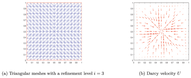
Figure 1 Pressure gradient at t = 0.0120 and the mesh used with h = 0.1188.

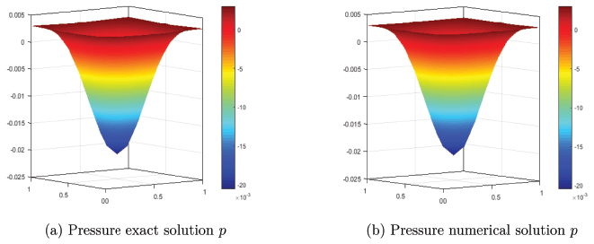
Figure 2 The exact and numerical solutions of the pressure equation at t = 0.0120.

Figure 3 The exact and numerical solutions of the concentration equation at t = 0.0120.

The surface plots for the pressure, the gradient of the pressure and the concentration of the invading fluid at t = 10⁻³ with the step of the mesh is h = 0.1188 are presented respectively in Figures 1(b)–3(b). The Tables 3, 4 and 5 are present respectively the norms L¹(Ω), L²(Ω) and L^∞(Ω) between the exact solution and the numerical solution of the pressure and the concentration, these norms are defined by the following formulas:

$$\{\begin{array}{l}\mathit{errl}1={\Vert u_T-u(x)\Vert }_{L^1(\Omega )}={\displaystyle \sum _{𝒦\in ℳ}}{m}_{𝒦}|u_{𝒦}-u(x_{𝒦})|,\hfill \\ \mathit{errl}2={\Vert u_T-u(x)\Vert }_{L^2(\Omega )}={\left(\frac{{\displaystyle \sum _{𝒦\in ℳ}}{m}_{𝒦}|u_{𝒦}-u(x_{𝒦}){|}^2}{{\displaystyle \sum _{𝒦\in ℳ}}{m}_{𝒦}|u(x_{𝒦}){|}^2}\right)}^{1/2},\hfill \\ \mathit{errlinf}={\Vert u_{𝒯}-u(x)\Vert }_{L^{\infty }(\Omega )}=\underset{𝒦\in ℳ}{{\displaystyle \max }}|u_{𝒦}-u(x_{𝒦})|.\hfill \end{array}$$

(77)

with u_𝒯 is the numerical solution and u(x) is the exact solution.

Table 3 L¹ − norm Convergence results of the SUSHI method on the pressure p and concentration c at t = 10⁻³

Level	N.U	Step	‖p − pext‖L1(Ω)	Order	‖c − cext‖Ll(Ω)	Order
1	56	0.4751	4.5716e-05	–	0.007	–
2	212	0.2375	1.2788e-05	1.1275	0.0018	1.3184
3	824	0.1188	3.2903e-06	1.1205	4.5244e-04	1.2572
4	3248	0.0594	9.2565e-07	1.1005	5.0308e-05	1.2709
5	12896	0.0297	4.0595e-07	1.0593	6.4287e-06	1.0569

Table 4 L² − norm Convergence results of the SUSHI method on the pressure p and concentration c at t = 10⁻³

Level	N.U	Step	‖p − pext‖L2(Ω)	Order	‖c − cext‖L2(Ω)	Order
1	56	0.4751	5.1180e-05	–	0.0086	–
2	212	0.2375	1.5027e-05	1.1240	0.0022	1.3353
3	824	0.1188	3.9538e-06	1.1202	5.6307e-04	1.2708
4	3248	0.0594	1.1598e-06	1.0986	5.8721e-05	1.2931
5	12896	0.0297	5.7188e-07	1.0517	1.0516e-06	1.0163

Table 5 L^∞ – norm Convergence results of the SUSHI method on the pressure p and concentration c at t = 10⁻³

Level	N.U	Step	‖p − pext‖L∞(Ω)	Order	‖c − cext‖L∞(Ω)	Order
1	56	0.4751 0.0014	–	0.0602	–
2	212	0.2375	8.0704e-04	1.0838	0.0329	1.2150
3	824	0.1188	5.2442e-04	1.7468	0.0157	1.2167
4	3248	0.0594	8.2744e-05	0.5705	0.0083	1.2533
5	12896	0.0297	7.9262e-05	1.0039	9.8790e-04	1.2314

And to calculate the order of convergence, let or1, or2 and orinf are the orders of convergence, they are defined by for i ≥ 2:

$$\{\begin{array}{l}\mathit{or}1=\frac{\mathit{ln}(\mathit{errl}{1}_i)}{\mathit{ln}(\mathit{errl}{1}_{i-1})},\hfill \\ \mathit{or}2=\frac{\mathit{ln}(\mathit{errl}{2}_i)}{\mathit{ln}(\mathit{errl}{2}_{i-1})},\hfill \\ \mathit{orinf}=\frac{\mathit{ln}({\mathit{errlinf}}_i)}{\mathit{ln}({\mathit{errlinf}}_{i-1})}.\hfill \end{array}$$

3.1.3 Test 3 (Peaceman model with continuous permeability)

In this numerical test, the spatial domain is Ω = (0,1000) × (0,1000)ft², and the time period is [0, 3600] days. The injection and the production well are respectively located at the upper-right corner (1000, 1000) and the lower-left corner (0, 0) with an injection rate q⁺ = 30ft²/day and a production rate q⁻ = 30ft²/day. The viscosity of the oil is μ(0) = 1.0cp, the injection concentration is $\widehat{c}=1.0$. The initial concentration is c₀(x) = 0 and the porosity of the medium is specified as ϕ(x) = 0.1. We consider that the porous medium is homogeneous and isotropic and the permeability tensor is given by K = 80I with I is the identity matrix. Let M = 1, and μ(c) = 1.0cp. We assume that ϕd_m = 1.0ft²/day, ϕd_l = 5.0ft and ϕd_t = 0.5ft. on an unstructured mesh (4), we present the pressure and the speed (5) and the concentration at the different values of t in the Figures 6(a)–6(f).

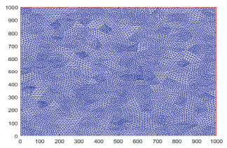
Figure 4 Triangular mesh used with a refinement level i = 5.

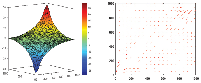
Figure 5 The pressure (left) and the gradient of the pressure (right) at t = 3600 days.

3.1.4 Test 4 (Peaceman model with discontinuous permeability)

Later, let c₀(x) = 0 and the porosity of the medium is specified as ϕ(x) = 0.1. We consider that the porous medium is homogeneous and isotropic and the permeability tensor is given by K = (801_y<500+201_y>500)I. Let M = 1, and μ(c) = 1.0cp. We assume that ϕd_m = 1.0ft²/day, ϕd_l = 5.0ft and ϕd_t = 0.5ft. In a structured mesh (7a) we calculate the norm V defined in Figure 7(b) in each step time and we remark in the Table 6 that ∑_𝒦∈ℳ m_𝒦p𝒦 close to zeros.

3.1.5 Test 5 (Peaceman model with an adverse mobility ratio)

In this test case, we are interested in the case where the relation between the equation of the pressure and that of the concentration is strong with a discontinuity of the permeability K(x, c), i.e μ(c) = (1 + (M^1/4 − 1)c)⁻⁴ with M = 41 and if (x, y) ∈ [200, 400] × [200, 400] ∪ [600, 800] × [200, 400] ∪ [200, 400] × [600, 800] ∪ [600, 800] × [600, 800], K(x, y) = 80 else K(x, y) = 20. Let c₀(x) = 0 and the porosity of the medium is specified as ϕ(x) = 0.1, and we assume that ϕd_m = 0ft²/day, ϕd_l = 5.0ft and ϕd_t = 0.5ft.

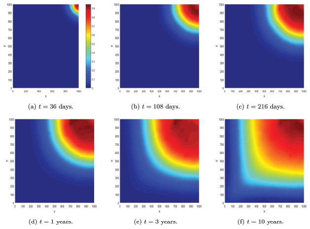
Figure 6 Surfaces plot of concentration, at different value of t, with δt = 36 days and the mesh of the domain is made of 928 triangles of maximal edge length 50ft.

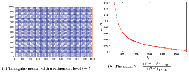
Figure 7 Norm V of concentration (7b) and structured triangular meshes (7a).

Table 6 The value of the integral of the pressure ∫_Ωp(x)dx at t = 3600, with K = (801_y<500 + 201_y>500)I

Refinement level	${\displaystyle \sum _{𝒦\in ℳ}{m}_{𝒦}{p}_{𝒦}}$
1	4.330e-01
2	1.083e-01
3	2.76e-02
4	7e-03
5	1.8e-03

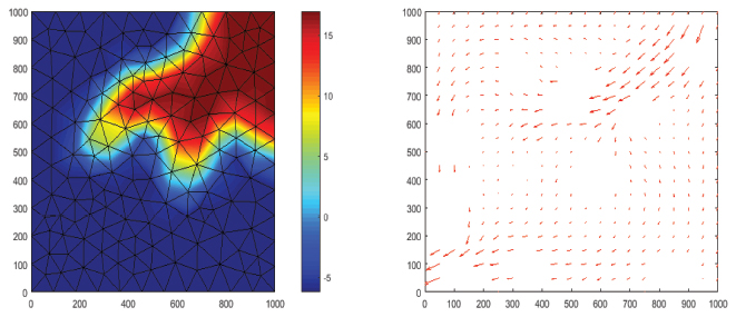
Figure 8 The pressure (left) and the gradient of the pressure (right) at t = 3600days ≈ 10years.

The Figure 8 represents the pressure and the pressure gradient at t = 10 years, and the Figure 9 represents the surfaces plot of concentration, at t = 36 days, t ≃ 1 years, t ≃ 3 years and t ≃ 10 years, with δt = 36 days.

3.2 Analysis Convergence

Theorem 3.1 Let 𝒟_m be a family of discretisation in the sense of Definition (2.1), for any 𝒟 ∈ 𝒟_m, let ℬ ∈ ℰ_int and $({\beta }_{\sigma }^{𝒦})$ satisfying by (18). Assume that there exists θ > 0 such that θ_𝒟,ℬ < θ for all 𝒟 ∈ 𝒯, where θ_𝒟ℬ is defined by (33). Let (δt_m)_m≤1 be a sequence of time steps such that T/δt_m is an integer and δt_m → 0 as m → +∞.

Then, the Scheme (72) defines a sequence of approximation solution (p_m = p_𝒟m,δtm, U_m = U_𝒟m,δtm, c_m = c_𝒟m,δtm) ∈ X_𝒯m,δtm × X_𝒟m,δtm × X_𝒯m,δtm, there exists $\overline{p}\in L^{\infty }(0,T;H^1(\Omega ))$, Ū ∈ L^∞(0,T; L²(Ω)), $\overline{c}\in L^{\infty }(0,T;L^2(\Omega ))$, and, up to a subsequence, we have the following convergence results when m → infin;

$$\begin{array}{l}{p}_m\to \overline{p}\mathit{weakly}-*\mathit{in}{L}^{\infty }(0,T;L^2(\Omega ))\mathit{and\; strongly\; in}\hfill \\ L^p(0,T;L^q(\Omega )),\forall p<\infty ,q<2;\hfill \end{array}$$ $$\begin{array}{l}{\nabla }^{h_m}{p}_m\to \nabla \overline{p}\mathit{weakly}-*\mathit{in}{(L^{\infty }(0,T;L^2(\Omega )))}^2\mathit{and\; strongly\; in}\hfill \\ {(L^2((0,T)\times \Omega ))}^2;\hfill \end{array}$$

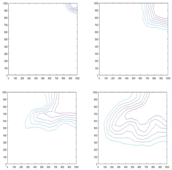
Figure 9 Surfaces plot of concentration, at t = 36 days, t ≃ 1 years, t ≃ 3 years and t ≃ 10 years, with δt = 36 days.

$$\begin{array}{l}{U}_m\to \overline{U}\mathit{weakly}-*\mathit{in}{(L^{\infty }(0,T;L^2(\Omega )))}^2\mathit{and\; strongly\; in}\hfill \\ {(L^2((0,T)\times \Omega ))}^2;\hfill \end{array}$$ $$\begin{array}{l}{c}_m\to \overline{c}\mathit{weakly}-*\mathit{in}{L}^{\infty }(0,T;L^2(\Omega ))\mathit{and\; strongly\; in}\hfill \\ L^p(0,T;L^q(\Omega )),\forall p<\infty ,q<2;\hfill \end{array}$$ $${\nabla }^{h_m}{c}_m\to \nabla \overline{c}\mathit{weakly\; in}{L}^2((0,T)\times \Omega ){)}^2.$$

Moreover, (p¯,U¯,c¯) is a weak solution to (1–2).

3.2.1 Convergence of the pressure

Lemma 3.2 Let F be a family of discretisation in the sense of Definition 2.1. Let δt_m be a sequence of times steps such that T/δt_m is an integer and δt_m → 0 as m → ∞. We consider a sequence of functions (v_m)_m with v_m = v_𝒟m,δtm ∈ X_𝒟m,δt when m → ∞ such that

$$\begin{array}{l}{\upsilon }_m\to \upsilon \mathit{weakly\; in}{L}^2((0,T)\times \Omega ),\hfill \\ (\mathit{respectively\; weakly-}*\mathit{in}{L}^{\infty }(0,T;L^2(\Omega )))\hfill \end{array}$$ $$\begin{array}{l}{\nabla }_{{𝒟}_m}{\upsilon }_m\to \chi \mathit{weakly\; in}{(L^2((0,T)\times \Omega ))}^2,\hfill \\ (\mathit{respectively\; weakly-}*\mathit{in}{L}^{\infty }(0,T;L^2(\Omega ))).\hfill \end{array}$$

Then, we have

$$\nabla \upsilon =\chi \mathit{and}\upsilon \in L^2(0,T;H^1(\Omega ))(\mathit{respectively\; in}{L}^{\infty }(0,T;H^1(\Omega )))$$

Proof 3.3 An adaptation of the proof of Lemma 4.2 in [20], leads to prove that ∇v = χ in the distribution sense on ]0,T[×Ω, and therefore v ∈ L² (0,T; H¹(Ω)) or v ∈ L^∞((0,T) × Ω).

Lemma 3.4 Under the assumptions of Theorem (3.1), there exists $\overline{p}\in L^{\infty }(0,T;H^1(\Omega ))$ and Ū ∈ (L^∞(0,T; L²(Ω)))², such that the sequences (p_m)_m, (U_m)_m defined by the Scheme (72) have the following convergence result when m → ∞

$$\begin{array}{l}{p}_m\to \overline{p}\mathit{weakly}-*\mathit{in}{L}^{\infty }(0,T;L^2(\Omega ))\hfill \\ \mathit{and\; strongly\; in}{L}^p(0,T;L^q(\Omega )),\forall p<\infty ,q<2;\hfill \end{array}$$ $$\begin{array}{l}{\nabla }^{h_m}{p}_m\to \nabla \overline{p}\mathit{weakly}-*\mathit{in}{(L^{\infty }(0,T;L^2(\Omega )))}^2\hfill \\ \mathit{and\; strongly\; in}{(L^2((0,T)\times \Omega ))}^2;\hfill \end{array}$$ $$\begin{array}{l}{U}_m\to \overline{U}\mathit{weakly}-*\mathit{in}{(L^{\infty }(0,T;L^2(\Omega )))}^2\hfill \\ \mathit{and\; strongly\; in}{(L^2((0,T)\times \Omega ))}^2;\hfill \end{array}$$

and ($(\overline{p},\overline{U})$, Ū) is a weak solution to (1).

Proof 3.5 step 1: Using Lemma 2.16 (a priori estimate), we get when m → ∞

$$\begin{array}{l}{p}_m\to \overline{p}\mathit{weakly-}*\mathit{in}{L}^{\infty }(0,T;L^2(\Omega ));\hfill \\ {\nabla }_{h_m}{p}_m\to \upsilon \mathit{weakly-}*\mathit{in}{(L^{\infty }(0,T;L^2(\Omega )))}^2;\hfill \\ U_m\to \tilde{U}\mathit{weakly-}*\mathit{in}{(L^{\infty }(0,T;L^2(\Omega )))}^2;\hfill \end{array}$$

Lemma 3.2 implies that

$$\overline{p}\in L^{\infty }(0,T;H^1(\Omega )),\mathit{with}\nabla \overline{p}=\upsilon .$$

by (1), we have ∫_Ω p_m(t, .)dx = 0 for all t ∈]0,T[, it gives that ${\displaystyle {\int }_{\Omega }}\overline{p}(t,.)\mathit{dx}=0$ for all t ∈]0,T[. we define the function A_𝒟 : Ω × ℝ → M_d(ℝ) by A_𝒟(x, s) = A_𝒦(s) with s ∈ ℝ and x ∈ 𝒦. Let ĉ :]0,T[× → ℝ such that

$$\{\begin{array}{ll}\stackrel{⌣}{c}=c_{𝒦}^n,\hfill & \mathit{on}[n\delta t,(n+1)\delta t[\times 𝒦\mathit{with}n=0,\dots ,N;\hfill \\ \stackrel{⌣}{c}=c_{𝒦}^0,\hfill & \mathit{on}[0,\delta t[\times 𝒦;\hfill \\ \stackrel{⌣}{c}=c(.-\delta t,.),\hfill & \mathit{on}[\delta t,T[\times \Omega .\hfill \end{array}$$

We have $\stackrel{⌣}{c}\to \overline{c}$ in L¹(0,T; L¹(Ω)) as δt → 0 and h_d → 0. for all Z ∈ L²(]0,T[×Ω)^d, ${\displaystyle {\int }_0^T}{\displaystyle {\int }_{\Omega }}Z.U={\displaystyle {\int }_0^T}{\displaystyle {\int }_{\Omega }}-A_{𝒟}{(.,\stackrel{⌣}{c})}^{T}Z.v$ with $U=-A_{𝒟}(.,\stackrel{⌣}{c}).\upsilon$. Using Lemma 7.6 in [12], we get ${\displaystyle {\int }_0^T}{\displaystyle {\int }_{\Omega }}Z.U\to {\displaystyle {\int }_0^T}{\displaystyle {\int }_{\Omega }}-A_{𝒟}{(.,c)}^{T}Z.\nabla \overline{p}$. That’s give Ū = Ũ.

Let $\Psi \in C_c^2(]0,T[\times \Omega )$ such that

$${𝒫}_{𝒟,ℬ}{\Psi }^n=\{\begin{array}{ll}{\Psi }^n(x_{𝒦}),\hfill & \mathit{for\; all}𝒦\in ℳ\hfill \\ {\Psi }^n(x_{\sigma }),\hfill & \mathit{for\; all}\sigma \in \mathscr{H}\hfill \\ {\displaystyle {\sum }_{𝒦\in ℳ}{\beta }_{\sigma }^{𝒦}{\Psi }^n(x_{𝒦}),}\hfill & \mathit{for\; all}\sigma \in ℬ\hfill \\ {\Psi }^n(x_{𝒦}),\hfill & \mathit{for\; all}\sigma \in {ℰ}_{\mathit{ext}}.\hfill \end{array}$$

Let us take v = 𝒫_𝒟,ℬΨ in (50), we get

$${\displaystyle {\int }_0^T}{\displaystyle {\int }_{\Omega }}A(x,c){\nabla }_{{𝒟}_m}{p}_m.{\nabla }_{{𝒟}_m}{𝒫}_{𝒟,ℬ}\Psi \mathit{dxdt}={\displaystyle {\int }_0^T}{\displaystyle {\int }_{\Omega }}{𝒫}_{𝒟,ℬ}\Psi (q^{+}-q^{-})\mathit{dxdt}.$$

(78)

Since ${\nabla }_{{𝒟}_m}{p}_m\to \nabla \overline{p}$ weakly in L^∞(0,T; L²(Ω))² and the consistency of the discret gradient, we have

$${𝒫}_{𝒟,ℬ}\Psi \to \nabla \Psi$$

Hence

$$\begin{array}{l}\underset{h_{{𝒟}_m}\to 0}{{\displaystyle \lim }}{\displaystyle {\int }_0^T}{\displaystyle {\int }_{\Omega }}A(x,c){\nabla }_{{𝒟}_m}{p}_m.{\nabla }_{{𝒟}_m}{𝒫}_{𝒟,ℬ}\Psi \mathit{dxdt}\hfill \\ ={\displaystyle {\int }_0^T}{\displaystyle {\int }_{\Omega }}A(x,c)\nabla \overline{p}.\nabla \Psi \mathit{dxdt}.\hfill \end{array}$$

Therefore, p is the unique solution of (13), and we get that the whole family (p_𝒟)_𝒟∈ℱ converges to p as h_𝒟 → 0.

step 2: Let $\psi \in C_c^{\infty }(]0,T[\times \Omega )$ be begin. Thanks to the Cauchy-Schwartz inequality, we have

$${\displaystyle {\int }_0^T}{\displaystyle {\int }_{\Omega }}|{\nabla }_{𝒟}{p}_{𝒟}(x)-\nabla p(x){|}^2\mathit{dx}\le 3(T_5^{𝒟}+T_6^{𝒟}+T_7),$$

(79)

with

$$T_5^{𝒟}={\displaystyle {\int }_0^T}{\displaystyle {\int }_{\Omega }}|{\nabla }_{𝒟}{p}_{𝒟}(x)-{\nabla }_{𝒟}{𝒫}_{𝒟}\psi (x){|}^2\mathit{dxdt},$$

(80)

$$T_6^{𝒟}={\displaystyle {\int }_0^T}{\displaystyle {\int }_{\Omega }}|{\nabla }_{𝒟}{𝒫}_{𝒟}\psi (x)-\nabla \psi (x){|}^2\mathit{dxdt},$$

(81)

and

$$T_7={\displaystyle {\int }_0^T}{\displaystyle {\int }_{\Omega }}|\nabla \psi (x)-\nabla p(x){|}^2\mathit{dxdt}.$$

(82)

Thanks to lemma of consistence in [20], we have ${{\displaystyle \lim }}_{h_{𝒟}\to 0}{T}_6^{𝒟}=0$. Thanks to Lemma 2.7 there exists C₇ such that

$$\left|\right|{\nabla }_{𝒟}w|{|}_{L(0,T;L^2{(\omega )}^d)}^2\le C_5|w{|}_{𝒟,\delta t}^2\le C_7{[w,w]}_{F^1},\forall w\in X_{𝒟}.$$

(83)

With $C_7=\frac{C_5}{{\alpha }_K}$. Taking w = p_m − 𝒫_𝒟ψ, we have

$$T_5^{𝒟}\le C_7{[p_m-{𝒫}_{𝒟}\psi ,p_m-{𝒫}_{𝒟}\psi ]}_{F^1}.$$

(84)

By step 1, we get

$$\underset{h_{𝒟}\to 0}{{\displaystyle \lim }}{[p_m-{𝒫}_{𝒟}\psi ,p_m-{𝒫}_{𝒟}\psi ]}_{F^1}={\displaystyle {\int }_0^T}{\displaystyle {\int }_{\Omega }}\nabla (p-\psi ).K(x,c)\nabla (p-\psi )(x)\mathit{dxdt}.$$

(85)

Thats gives

$$\underset{h_{𝒟}\to 0}{{\displaystyle \lim }}{[p_m-{𝒫}_{𝒟}\psi ,p_m-{𝒫}_{𝒟}\psi ]}_{F^1}\le \overline{\lambda }{\displaystyle {\int }_0^T}{\displaystyle {\int }_{\Omega }}|\nabla p(x)-\nabla \psi (x){|}^2\mathit{dxdt}.$$

which yields

$$\underset{h_{𝒟}\to 0}{{\displaystyle \lim }}\sup T_5^{𝒟}\le C_7\overline{\lambda }{\displaystyle {\int }_0^T}{\displaystyle {\int }_{\Omega }}|\nabla p(x)-\nabla \psi (x){|}^2\mathit{dx}.$$

(86)

Then, there exists C₈ independent of 𝒟, such that

$$\begin{array}{l}{\displaystyle {\int }_0^T}{\displaystyle {\int }_{\Omega }}|{\nabla }_{𝒟}{p}_{𝒟}(x)-\nabla p(x){|}^2\mathit{dx}\le C_7{\displaystyle {\int }_0^T}{\displaystyle {\int }_{\Omega }}|\nabla \psi (x)-\nabla p(x){|}^2\mathit{dx}+3T_7^{𝒟}.\hfill \\ \le C_8{\displaystyle {\int }_0^T}{\displaystyle {\int }_{\Omega }}|\nabla \psi (x)-\nabla p(x){|}^2\mathit{dx}.\hfill \end{array}$$

We may choose ψ such that ${\displaystyle {\int }_0^T}{\displaystyle {\int }_{\Omega }}|\nabla \psi (x)-\nabla p(x)|\mathit{dx}\le \varepsilon$ and h_𝒟 small enough, then

$$\underset{h_{𝒟}\to 0}{{\displaystyle \lim }}{\displaystyle {\int }_0^T}{\displaystyle {\int }_{\Omega }}|{\nabla }_{𝒟}{p}_{𝒟}(x)-\nabla p(x){|}^2\mathit{dxdt}=0.$$

(87)

Hence, we have the strongly convergent of ${\nabla }_{𝒟}{p}_m\to \nabla \overline{p}$. That’s implies: U_m → Ū.

Then we have the proof.

3.2.2 Convergence of the concentration

Lemma 3.6 (compactness concentration) Under the assumption of Theorem (3.1), c is relatively compact in $L^1(0,T;L_{\mathit{Loc}}^1(\Omega ))$.

Proof 3.7 step 1: Let $\tilde{c}:[0,T]\times \Omega \to ℝ$ continuous function in time and affine on each time interval. Hence, for all n = 0; ..., N − 1 and all t ∈ [nδt, (n + 1)δt],

$$\tilde{c}(t,.)=\frac{t-n\delta t}{\delta t}{c}_{𝒦}^{n+1}+\frac{(n+1)\delta t-t}{\delta t}{c}_{𝒦}^n\mathit{on}𝒦.$$

Let $w\in C_c^2(\Omega )$ and n ∈ {0, ..., N − 1}. Multiplying (58) by w_𝒦, we get

$$\begin{array}{l}{\displaystyle {\int }_{\Omega }}{\phi }_{𝒟}(x){\partial }_t\tilde{c}(t,x)w(x)\mathit{dx}\hfill \\ =<{\phi }_{𝒦}\frac{c_{𝒦}^{n+1}-c_{𝒦}^n}{\delta t},w_{𝒦}>\hfill \\ =<{\mathit{div}}_{𝒦}(𝒟{\nabla }_{𝒟}{c}_{𝒦}^{n+1}),w_{𝒦}>-<{\mathit{divc}}_{\sigma }(U_{𝒟}^{n+1},c_{𝒦}^{n+1}),w_{𝒦}>-\hfill \\ <q_{𝒦}^{-,n+1}{c}_{𝒦}^{n+1},w_{𝒦}>+<q_{𝒦}^{+,n+1}{\widehat{c}}_{𝒦}^{n+1},w_{𝒦}>\text{}.\hfill \end{array}$$

Let

$$T_1=<{\mathit{div}}_{𝒦}(𝒟{\nabla }_{𝒟}{c}_{𝒦}^{n+1}),w_{𝒦}>,$$

(88)

$$=-<D_{𝒟}(U_{𝒟}^{n+1}){\nabla }_{𝒟}{c}_{𝒦}^{n+1},{\nabla }_{𝒟}{w}_{𝒦}>,$$

(89)

$$=-{\displaystyle \sum _{𝒦\in M}}{\displaystyle \sum _{\sigma \in {ℰ}_{𝒦}}}{m}_{𝒦}{𝒟}_{𝒦}(U_{𝒦}^{n+1}){\nabla }_{𝒦,\sigma }{c}_{𝒦}^{n+1}.{\nabla }_{𝒦,\sigma }{w}_{𝒦}.$$

(90)

Then, the hypothesis (9) on D implies

$$\left|T_1\right|\le {\Lambda }_{𝒟}|w{|}_X{\displaystyle \sum _{𝒦\in M}}{\displaystyle \sum _{\sigma \in {ℰ}_{𝒦}}}{m}_{𝒦}(1+\left|U_{𝒦}^{n+1}\right|)|{\nabla }_{𝒦,\sigma }{c}_{𝒦}^{n+1}|.$$

(91)

The second term

$$\begin{array}{l}{T}_2=-<{\mathit{divc}}_{\sigma }(U_{𝒟}^{n+1},c_{𝒦}^{n+1}),w_{𝒦}>,\hfill \\ =-{\displaystyle \sum _{𝒦\in M}}{\displaystyle \sum _{\sigma \in {ℰ}_{𝒦}}}{m}_{\sigma }\left({(U_{𝒟}^{n+1}.n_{𝒦,\sigma })}^{+}{c}_{𝒦}^{n+1}-{(U_{𝒟}^{n+1}.n_{𝒦,\sigma })}^{-}{c}_{ℒ}^{n+1}\right)w_{𝒦},\hfill \\ =-{\displaystyle \sum _{\sigma =𝒦/ℒ\in {ℰ}_{\mathit{int}}}}{m}_{\sigma }{\left(U_{𝒟}^{n+1}.n_{𝒦,\sigma }\right)}^{+}{c}_{𝒦}^{n+1}(w_{𝒦}-w_{ℒ})\hfill \\ -{\displaystyle \sum _{\sigma =𝒦/ℒ\in {ℰ}_{\mathit{int}}}}{m}_{\sigma }{\left(U_{𝒟}^{n+1}.n_{𝒦,\sigma }\right)}^{-}{c}_{𝒦}^{n+1}(w_{𝒦}-w_{ℒ}),\hfill \\ =-{\displaystyle \sum _{\sigma =𝒦/ℒ\in {ℰ}_{\mathit{int}}}}{m}_{\sigma }\left(U_{𝒟}^{n+1}.n_{𝒦,\sigma }\right)c_{𝒦}^{n+1}(w_{𝒦}-w_{ℒ})\hfill \\ -{\displaystyle \sum _{\sigma =𝒦/ℒ\in {ℰ}_{\mathit{int}}}}{m}_{\sigma }{\left(U_{𝒟}^{n+1}.n_{𝒦,\sigma }\right)}^{-}(c_{𝒦}^{n+1}-c_{ℒ}^{n+1})(w_{𝒦}-w_{ℒ}).\hfill \end{array}$$

That’s gives

$$\begin{array}{l}\hfill \left|T_2\right|\le \left|w{|}_X{\displaystyle \sum _{\sigma =𝒦/ℒ\in {ℰ}_{\mathit{int}}}}{d}_{𝒦,\sigma }\right|U_{𝒟}^{n+1}\left|\right|c_{𝒦}^{n+1}|+|w{|}_X\hfill \\ \hfill {\displaystyle \sum _{\sigma =𝒦/ℒ\in {ℰ}_{\mathit{int}}}}{d}_{𝒦,\sigma }\left|U_{𝒟}^{n+1}\right|\left|{\nabla }_{\sigma ,𝒦}{c}_{𝒦}^{n+1}\right|.\hfill \end{array}$$

(92)

We focus now on the last two terms $T_3=-<q_{𝒦}^{-,n+1}{c}_{𝒦}^{n+1},w_{𝒦}>$ and $T_4=<q_{𝒦}^{+,n+1}{\widehat{c}}_{𝒦}^{n+1},w_{𝒦}>$. They verify

$$\left|T_3\right|\le |w{|}_X{\Vert q^{-,n+1}\Vert }_{L^2(\Omega )}{\Vert c_{𝒟}^{n+1}\Vert }_{L^2(\Omega )}$$

(93)

$$\left|T_4\right|\le |w{|}_X{\Vert q^{+,n+1}\Vert }_{L^2(\Omega )}{\Vert {\widehat{c}}^{n+1}\Vert }_{L^2(\Omega )}$$

(94)

Finally we obtain for all w ∈ X_𝒟

$$\begin{array}{l}<{\phi }_{𝒦}\frac{c_{𝒦}^{n+1}-c_{𝒦}^n}{\delta t},w_{𝒦}>\hfill \\ \le |w{|}_X({\Lambda }_{𝒟}{\displaystyle \sum _{𝒦\in M}}{\displaystyle \sum _{\sigma \in {ℰ}_{𝒦}}}{m}_{𝒦}(1+|U_{𝒦}^{n+1}|)\left|{\nabla }_{𝒦,\sigma }{c}_{𝒦}^{n+1}\right|\hfill \\ +{\displaystyle \sum _{\sigma =𝒦/ℒ\in {ℰ}_{\mathit{int}}}}{d}_{𝒦,\sigma }\left|U_{𝒟}^{n+1}\right|\left|c_{𝒦}^{n+1}\right|\hfill \\ +{\displaystyle \sum _{\sigma =𝒦/ℒ\in {ℰ}_{\mathit{int}}}}{d}_{𝒦,\sigma }\left|U_{𝒟}^{n+1}\right|\left|{\nabla }_{\sigma ,𝒦}{c}_{𝒦}^{n+1}\right|\hfill \\ +{\Vert q^{+,n+1}\Vert }_{L^2(\Omega )}{\Vert {\widehat{c}}_{𝒟}^{n+1}\Vert }_{L^2(\Omega )}+{\Vert q^{-,n+1}\Vert }_{L^2(\Omega )}{\Vert c_{𝒟}^{n+1}\Vert }_{L^2(\Omega )}).\hfill \end{array}$$

Multiplying by δt and summing over n we get

$$\begin{array}{l}{\displaystyle \sum _{n=0}^{N-1}}\delta t{\Vert \phi \partial {\tilde{c}}_{𝒟}^{n+1}\Vert }_{(C_c^2(\Omega ){)}^{\prime }}\hfill \\ \le {\Lambda }_D{\displaystyle \sum _{n=0}^{N-1}}\delta t{\displaystyle \sum _{𝒦\in ℳ}}{\displaystyle \sum _{\sigma \in {ℰ}_{𝒦}}}{m}_{𝒦}(1+|U_{𝒦}^{n+1}|)\left|{\nabla }_{𝒦,\sigma }{c}_{𝒦}^{n+1}\right|\hfill \\ +{\displaystyle \sum _{n=0}^{N-1}}\delta t{\displaystyle \sum _{\sigma =𝒦/ℒ\in {ℰ}_{\mathit{int}}}}{d}_{𝒦,\sigma }\left|U_{𝒟}^{n+1}\right|\left|c_{𝒦}^{n+1}\right|\hfill \\ +{\displaystyle \sum _{n=0}^{N-1}}\delta t{\displaystyle \sum _{\sigma =𝒦/ℒ\in {ℰ}_{\mathit{int}}}}{d}_{𝒦,\sigma }\left|U_{𝒟}^{n+1}\right|\left|{\nabla }_{\sigma ,𝒦}{c}_{𝒦}^{n+1}\right|\hfill \\ +{\displaystyle \sum _{n=0}^{N-1}}\delta t{\Vert q^{-,n+1}\Vert }_{L^2(\Omega )}{\Vert c_{𝒟}^{n+1}\Vert }_{L^2(\Omega )}\hfill \\ +{\displaystyle \sum _{n=0}^{N-1}}\delta t{\Vert q^{+,n+1}\Vert }_{L^2(\Omega )}{\Vert {\widehat{c}}_{𝒟}^{n+1}\Vert }_{L^2(\Omega )}.\hfill \end{array}$$

Using the Cauchy-Schwartz inequality and Lemma 4.3, then we have ${\partial }_t({\phi }_{𝒟}\tilde{c})$ is bounded in $L^2(0,T;(C_c^2(\Omega ){)}^{\prime })$. $\tilde{c}$ and φ_𝒟 are respectively bounded in L^∞(0,T; L²(Ω)) and L²(Ω), that’s implies ${\phi }_{𝒟}\tilde{c}$ is bounded in L^∞(0,T; L²(Ω)). ${\phi }_{𝒟}\tilde{c}$ is also bounded in $H^1(0,T;(C_c^2(\Omega ){)}^{\prime })(L^2(\Omega )$ is continuously embedded in $(C_c^2(\Omega ){)}^{\prime }$ and L^∞(Ω) is continuously embedded in L²(Ω)). In the fact L²(Ω) is compactly embedded in $(C_c^2(\Omega ){)}^{\prime }$ and using Aubin’s compactness theorem proved by Gallouet and Latché [22] we deduce that ${\phi }_{𝒟}\tilde{c}$ is relatively compact in C([0,T]; $C([0,T];(C_c^2(\Omega ){)}^{\prime })$.

Step 2: ${\phi }_{𝒟}c(t,.)={\phi }_{𝒟}\tilde{c}(n\delta t,.)$ on Ω. $H^1(0,T;(C_c^2(\Omega ){)}^{\prime })$ is continuously embedded in $C^{1/2}([0,T];(C_c^2(\Omega ){)}^{\prime })$.

Hence, ${\phi }_{𝒟}\tilde{c}$ is also bounded in $C^{1/2}([0,T];(C_c^2(\Omega ){)}^{\prime })$ and there exists C not depending on δt or 𝒟 such that for all n = 0, ..., N − 1 and all t ∈ [nδt, (n + 1)δt],

$$\begin{array}{c}{\Vert {\phi }_{𝒟}c(t,.)-{\phi }_{𝒟}\tilde{c}(t,.)\Vert }_{(C_c^2(\Omega ){)}^{\prime }}={\Vert {\phi }_{𝒟}\tilde{c}((n+1)\delta t,.)-{\phi }_{𝒟}\tilde{c}(t,.)\Vert }_{(C_c^2(\Omega ){)}^{\prime }}\\ \le C_9\sqrt{\delta t}.\end{array}$$

Implies that as δt → 0, ${\phi }_{𝒟}c-\phi \tilde{c}\to 0$ in $L^{\infty }(0,T;(C_c^2(\Omega ){)}^{\prime })$. ${\phi }_{𝒟}\tilde{c}$ is relatively compact in $L^1(0,T;(C_c^2(\Omega ){)}^{\prime })$.

The Lemma 5.4 in [20] gives, for all ξ ∈ ℝ

$${\Vert c(t,.+\xi )-c(t,.)\Vert }_{L^1({ℝ}^d)}\le \left|\xi \right|\sqrt{d}{\Vert c\Vert }_{1,1,ℳ}.$$

Integrating on t ∈ [nδt, (n + 1)δt[ and summing on n = 0, ..., N − 1, this implies

$${\Vert c(t,.+\xi )-c(t,.)\Vert }_{L^1(]0,T[\times {ℝ}^d)}\le \left|\xi \right|\sqrt{d}{\displaystyle \sum _{n=0}^{N-1}}{\Vert c\Vert }_{1,1,ℳ}.$$

(95)

Thanks to the estimates of Lemma 4.3 we have

$${\Vert c(t,.+\xi )-c(t,.)\Vert }_{L^1({ℝ}^d)}\to 0\mathit{as}\xi \to 0\mathit{independently\; of}\delta t\mathit{and}𝒟.$$

(96)

Since φ_𝒟 and c are respectively bounded in L^∞(Ω) and L^∞(0,T; L²(Ω)), and using the estimates of Lemma 4.3 we have

$$\begin{array}{l}{\Vert ({\phi }_{𝒟}c)(.,.+\xi )-({\phi }_{𝒟}c)\Vert }_{L^1(]0,T[\times {ℝ}^d)}\hfill \\ ={\Vert {\phi }_{𝒟}(.+\xi )(c(.,.+\xi )-c)+({\phi }_{𝒟}(.+\xi )-{\phi }_{𝒟})c\Vert }_{L^1(]0,T[\times {ℝ}^d)}\hfill \\ \le C{\Vert c(.,.+\xi )-c\Vert }_{L^1(]0,T[\times {ℝ}^d)}+C{\Vert {\phi }_{𝒟}(.+\xi )-{\phi }_{𝒟}\Vert }_{L^1(]0,T[\times {ℝ}^d)}.\hfill \end{array}$$

φ_𝒟 → φ in L²(Ω) as h_𝒟 → 0, the propriety ‖φ_𝒟(. + ξ) − φ_𝒟‖_L²(ω → 0 as ξ → 0 and (95) implies that ‖φ_𝒟c(.,. + ξ) − φ_𝒟c‖_{L¹(0,T;L¹(ω))} → 0 as ξ → 0 independently of 𝒟 and δt. Using Lemma 2.14 and the fact that φ_𝒟c → is relatively compact in $L^1(0,T;(C_c^2(\Omega ){)}^{\prime })$, we get φ_𝒟c is relatively compact in $L^1(0,T;L_{\mathit{Loc}}^1(\Omega ))$. Let $f\in L^1(0,T;L_{\mathit{Loc}}^1(\Omega ))$ such that φ_𝒟c → f in $L^1(0,T;L_{\mathit{Loc}}^1(\Omega ))$ as δt → 0 and h_𝒟 → 0. Hence, the hypotheses (6) and the dominated convergence theorem then shows that $c=\frac{1}{{\phi }_{𝒟}}{\phi }_{𝒟}c\to \frac{1}{\phi }f$ in $L^1(0,T;L_{\mathit{Loc}}^1(\Omega ))$ (we also using the fact that φ_𝒟 → φ in L²(Ω)), which concludes the proof.

Lemma 3.8 Under the assumptions of Theorem (3.1), the function $\overline{c}$. Ū introduced in (3.4) satisfy (13).

Proof 3.9 Let $\psi \in C^{\infty }([0,T]\times \overline{\Omega })$, multiplying (58) by ψⁿ(x_𝒟) and sum on 𝒟 ∈ ℳ and on n = 0, ..., N − 1, we get

$$T_6+T_7+T_8+T_9=T_{10}.$$

With

$$\begin{array}{l}{T}_6={\displaystyle \sum _{n=0}^{N-1}}\delta t{\displaystyle \sum _{𝒦\in ℳ}}{m}_{𝒦}{\phi }_{𝒦}\frac{c_{𝒦}^{n+1}-c_{𝒦}^n}{\delta t}{\psi }^{n+1}(x_{𝒦}),\hfill \\ T_7=-{\displaystyle \sum _{n=0}^{N-1}}\delta t{\displaystyle \sum _{k\in ℳ}}{\displaystyle \sum _{\sigma \in {ℰ}_{𝒦}}}{ℱ}_{𝒦,\sigma }^2(c^{n+1}){\psi }^{n+1}(x_{𝒦}),\hfill \\ T_8={\displaystyle \sum _{n=0}^{N-1}}\delta t{\displaystyle \sum _{𝒦\in ℳ}}{\displaystyle \sum _{\sigma \in {ℰ}_{𝒦}}}{m}_{\sigma }{\mathit{divc}}_{\sigma }(c_{𝒟}^{n+1},U_{𝒟}^{n+1}){\psi }^{n+1}(x_{𝒦}),\hfill \\ T_9={\displaystyle \sum _{n=0}^{N-1}}\delta t{\displaystyle \sum _{𝒦\in ℳ}}{q}_{𝒦}^{-,n+1}{c}_{𝒦}^{n+1}{\psi }^{n+1}(x_{𝒦}),\hfill \\ T_{10}={\displaystyle \sum _{n=0}^{N-1}}\delta t{\displaystyle \sum _{𝒦\in ℳ}}{m}_{𝒦}{q}_{𝒦}^{+,n+1}{\widehat{c}}_{𝒦}^{n+1}{\psi }^{n+1}(x_{𝒦}).\hfill \end{array}$$

Limite of T₆:

$$\begin{array}{l}{T}_6={\displaystyle \sum _{n=0}^{N-1}}\delta t{\displaystyle \sum _{𝒦\in ℳ}}{m}_{𝒦}{\phi }_{𝒦}\frac{c_{𝒦}^{n+1}-c_{𝒦}^n}{\delta t}{\psi }^{n+1}(x_{𝒦}),\hfill \\ ={\displaystyle \sum _{n=0}^{N-1}}\delta t{\displaystyle \sum _{𝒦\in ℳ}}{m}_{𝒦}{\phi }_{𝒦}{c}_{𝒦}^{n+1}\frac{{\psi }_{𝒦}^{n+1}-{\psi }_{𝒦}^n}{\delta t}-{\displaystyle \sum _{𝒦\in ℳ}}{m}_{𝒦}{\phi }_{𝒦}{c}_{𝒦}^0{\psi }^1(x_{𝒦}),\hfill \\ ={\displaystyle {\int }_0^T}{\displaystyle {\int }_{\Omega }}\phi c{\xi }_{𝒦,𝒟}-{\displaystyle {\int }_{\Omega }}{\phi }_{𝒟}{c}_0{𝒫}_{ℳ}({\psi }^1).\hfill \end{array}$$

Where φ_𝒟 = φ_𝒦 on 𝒦, ${\xi }_{𝒦,𝒟}=\frac{{\psi }^{n+1}(x_{𝒦})-{\psi }^n(x_{𝒦})}{\delta t}$ on [(nδt, (n + 1)δt] × 𝒦 and ${𝒫}_{ℳ}({\psi }^1)={\psi }_{𝒦}^1$ on 𝒦. ψ is regular, then ξ_𝒦,𝒟 → −∂_tψ uniformly on [0,T] × Ω and 𝒫_𝒟(ψ¹) → ψ(0,.) uniformly on Ω; φ_𝒟 → φ strongly in L²(Ω). The weak-* convergence of c in L^∞(0,T; L²(Ω)) then implies

$$T_6\to {\displaystyle {\int }_0^T}{\displaystyle {\int }_{\Omega }}\phi \widehat{c}{\partial }_t\psi -{\displaystyle {\int }_{\Omega }}\phi c_0\psi (0,.).$$

(97)

Limit of T₇:

$$\begin{array}{l}{T}_7=-{\displaystyle \sum _{n=0}^{N-1}}\delta t{\displaystyle \sum _{𝒦\in ℳ}}{\displaystyle \sum _{\sigma \in {ℰ}_{𝒦}}}{F}_{𝒦,\sigma }^2(c^{n+1}){\psi }_{𝒦}^{n+1},\hfill \\ ={\displaystyle \sum _{n=0}^{N-1}}\delta t{\displaystyle \sum _{𝒦\in ℳ}}{\displaystyle \sum _{\sigma \in {ℰ}_{𝒦}}}{F}_{𝒦,\sigma }^2(c^{n+1})({\psi }_{𝒦}^{n+1}-{\psi }_{\sigma }^{n+1}),\hfill \\ ={\displaystyle \sum _{n=0}^{N-1}}\delta t{\displaystyle \sum _{𝒦\in ℳ}}{\displaystyle \sum _{\sigma \in {ℰ}_{𝒦}}}{\displaystyle \sum _{{\sigma }^{\prime }\in {ℰ}_{𝒦}}}{D}_{𝒦}^{\sigma ,{\sigma }^{\prime }}(c_{𝒦}^{n+1}-c_{{\sigma }^{\prime }}^{n+1})({\psi }_{𝒦}^{n+1}-{\psi }_{{\sigma }^{\prime }}^{n+1}),\hfill \\ ={\displaystyle {\int }_0^T}{\displaystyle {\int }_{\Omega }}{\nabla }_{𝒟}{c}^{n+1}D(x,U^n){\nabla }_{𝒟}{\psi }^{n+1}.\hfill \end{array}$$

Since U → Ū strongly in L²(]0,T[×Ω)^d, we have D(., U) → D(.,Ū) strongly in L²(]0,T[×Ω)^d×d (extract a subsequence of U which converges a.e. and use Vitali’s theorem). ∇_𝒟ψ → ∇ψ uniformly on ]0,T[×Ω, we deduce that D(., U)∇_𝒟ψⁿ⁺¹ → D(.,Ū)^T∇ ψ in L²(]0,T[×Ω)^d and the weak convergence of ${\nabla }_{𝒟}c\to \nabla \overline{c}$, we get

$$T_7\to {\displaystyle {\int }_0^T}{\displaystyle {\int }_{\Omega }}D\mathrm{<mo\; stretchy="false">(</mo>.,}U\mathrm{<mo\; stretchy="false">)</mo>}\nabla \overline{c}\mathrm{.}\nabla \psi \mathrm{.}$$

(98)

Limit of₈:

Applying the technic Using in proof of Lemma (3.6), we get

$$\begin{array}{l}{T}_8={\displaystyle \sum _{n=0}^{N-1}}\delta t{\displaystyle \sum _{𝒦\in ℳ}}{\displaystyle \sum _{\sigma \in {ℰ}_{𝒦}}}{m}_{\sigma }{\mathit{divc}}_{\sigma }(c_{𝒟}^{n+1},U_{𝒟}^{n+1}){\psi }_{𝒟}^{n+1},\hfill \\ ={\displaystyle \sum _{n=0}^{N-1}}\delta t{\displaystyle \sum _{\sigma =𝒦/ℒ\in {ℰ}_{\mathit{int}}}}{m}_{\sigma }\left(U_{𝒟}^{n+1}.n_{𝒦,\sigma }\right)c_{𝒦}^{n+1}({\psi }_{𝒦}^{n+1}-{\psi }_{ℒ}^{n+1})+\hfill \\ {\displaystyle \sum _{n=0}^{N-1}}\delta t{\displaystyle \sum _{\sigma =𝒦/ℒ\in {ℰ}_{\mathit{int}}}}{m}_{\sigma }{\left(U_{𝒟}^{n+1}.n_{𝒦,\sigma }\right)}^{-}(c_{𝒦}^{n+1}-c_{ℒ}^{n+1})({\psi }_{𝒦}^{n+1}-{\psi }_{ℒ}^{n+1}).\hfill \end{array}$$

That’s gives

$$\begin{array}{l}\left|T_8-{\displaystyle \sum _{n=0}^{N-1}}\delta t{\displaystyle \sum _{\sigma =𝒦/ℒ\in {ℰ}_{\mathit{int}}}}{m}_{\sigma }\left(U_{𝒟}^{n+1}.n_{𝒦,\sigma }\right)c_{𝒦}^{n+1}({\psi }_{𝒦}^{n+1}-{\psi }_{ℒ}^{n+1})\right|\hfill \\ =\left|{\displaystyle \sum _{n=0}^{N-1}}\delta t{\displaystyle \sum _{\sigma =𝒦/ℒ\in {ℰ}_{\mathit{int}}}}{m}_{\sigma }{\left(U_{𝒟}^{n+1}.n_{𝒦,\sigma }\right)}^{-}(c_{𝒦}^{n+1}-c_{ℒ}^{n+1})({\psi }_{𝒦}^{n+1}-{\psi }_{ℒ}^{n+1})\right|\text{},\hfill \\ \le {\Vert \psi \Vert }_{X_{𝒟,\delta t}}{\displaystyle \sum _{n=0}^{N-1}}\delta t{\displaystyle \sum _{\sigma \in ℰ}}{d}_{𝒦,\sigma }\left|U_{𝒟}^{n+1}\right|\left|{\nabla }_{\sigma ,𝒦}{c}_{𝒦}^{n+1}\right|.\hfill \end{array}$$

and

$${\displaystyle \sum _{n=0}^{N-1}}\delta t{\displaystyle \sum _{\sigma =𝒦/ℒ\in {ℰ}_{\mathit{int}}}}{m}_{\sigma }\left(U_{𝒟}^{n+1}.n_{𝒦,\sigma }\right)c_{𝒦}^{n+1}({\psi }_{𝒦}^{n+1}-{\psi }_{ℒ}^{n+1})\to {\displaystyle {\int }_0^T}{\displaystyle {\int }_{\Omega }}cU.\nabla \psi .$$

(99)

Using Lemma 2.18 and (99), we have

$$T_8\to {\displaystyle {\int }_0^T}{\displaystyle {\int }_{\Omega }}cU.\nabla \psi .$$

(100)

Limit of T₉ and T₁₀:

We have

$$T_9={\displaystyle \sum _{n=0}^{N-1}}\delta t{\displaystyle \sum _{𝒦\in M}}{q}_{𝒦}^{-,n+1}{c}_{𝒦}^{n+1}{\psi }^{n+1}(x_{𝒦})={\displaystyle {\int }_0^T}{\displaystyle {\int }_{\Omega }}{q}^{-}c{\psi }_{𝒟}\to {\displaystyle {\int }_0^T}{\displaystyle {\int }_{\Omega }}{q}^{-}\overline{c}\psi .$$

(101)

It is also easy to pass to the limit in

$$T_{10}={\displaystyle \sum _{n=0}^{N-1}}\delta t{\displaystyle \sum _{𝒦\in M}}{m}_{𝒦}{q}_{𝒦}^{+,n+1}{\widehat{c}}_{𝒦}^{n+1}{\psi }^{n+1}(x_{𝒦})={\displaystyle {\int }_0^T}{\displaystyle {\int }_{\Omega }}{q}^{+}{\widehat{c}}_{𝒟}{\psi }_{𝒟}.$$

The function ${\widehat{c}}_{𝒟,𝒦}$ equal to ${\widehat{c}}_{𝒦}^n$ on [nδt,(n + 1)δt[×Ω converges to $\widehat{c}$ in L²(]0,T[×Ω), then

$$T_{10}\to {\displaystyle {\int }_0^T}{\displaystyle {\int }_{\Omega }}{q}^{+}\widehat{c}\psi .$$

(102)

Using (97), (98), (100), (101), and (102) in T₆ + T₇ + T₈ + T₉ + T₁₀ we deduce that $\overline{c}$ is a weak solution to (13) with the function Ū limit of U.

Proof 3.10 The proof of Theorem 3.1 is a result of Lemma 3.4 and Lemma 3.8.

Acknowledgments

The authors would like to thank the referees for their careful reading of the paper and their valuable remarks.

References

[1] M. Rhoudaf, M. Mandari and O. Soualhi, The generalized finite volume SUSHI scheme for the discretisation of the peaceman model, (submitted)

[2] J. Douglas, J. R., The numerical simulation of miscible displacement, in Computational methods in nonlinear mechanics, (J. T. Oden, ED.), North Holland, Amsterdam, 1980.

[3] J. Bear, Dynamics of fluids in porous media, American Elsevier, 1972.

[4] J. Bear, A. Verruijt, Modelling Groundwater Flow and Pollution, 1987. 119. D. Reidel Publishing Company, Dordecht, Holland, 1995, pp. 473–502.

[5] J. Douglas, Jr., R. E. Ewing and M. F. Wheeler, Approximation of the pressure by a mixed method in the simulation of miscible displacement. R.A.I.R Anal. Numer., 17(1983), 17–33.

[6] P. H. Sammon, Numerical approximation for a miscible displacement in porous media. SIAM J. Numer. Anal. 23(1986), 505–542.

[7] J. Douglas, Jr., Numerical methods for the flow of miscible fluids in porous media, in Numerical methods in coupled system, (R.W. Lewis, P. Bettess, and E. Hinton, Eds.), Wiley, New York, 1984.

[8] J. Douglas, J. R. and J. E. Roberts, Numerical methods for model of compressible miscible displacement in porous media. Math. Comp. 41(1983), 441–459.

[9] X. Feng, On existence and uniqueness results for a coupled system modeling miscible displacement in porous media. J. Math. Anal. Appl., 194(3):883–910, 1995.

[10] C. Chainais-Hillairet, S. Krell and A. Mouton, Convergence analysis of a DDFV scheme for a system describing miscible fluid flows in porous media. Numerical Methods for Partial Differential Equations, Wiley, 2014, pp. 38.

[11] C. Chainais-Hillairet, S. Krell and A. Mouton, Study of discrete duality finite volume schemes for the peaceman model. SIAM J. Sci. Comput., 35(6):A2928–A2952, 2013.

[12] C. Chainais-Hillairet and J. Droniou, Convergence analysis of a mixed finite volume scheme for an elliptic-parabolic system modeling miscible fluid flows in porous media. SIAM J. Numer. Anal., 45(5):2228–2258 (electronic), 2007.

[13] H. Hu, Y. Fu and J. Zhou, Numerical solution of a miscible displacement problem with dispersion term using a two-grid mixed finite element approach. Numer. Algor., 2019, 81(3), 879–914.

[14] J. Jaffré and J. E. Roberts, Upstream weighting and mixed finite elements in the simulation of miscible displacements. RAIRO Model. Math. Anal. Numer., 19(3):443–460, 1985.

[15] J. Douglas, R. E. Ewing and M. F. Wheeler, A time-discretization procedure for a mixed finite element approximation of miscible displacement in porous media. RAIRO Anal. Num., 17 (1983), 249–265.

[16] S. Bartels, M. Jensen and R. Muller, Discontinuous Galerkin finite element convergence for incompressible miscible displacement problems of low regularity. SIAM J. Numer. Anal., 47(5):3720–3743, 2009.

[17] R. E. Ewing, T. F. Russell and M. F. Wheeler, Simulation of miscible displacement using mixed methods and a modified method of characteristics. SPE, 12241:71–81, 1983.

[18] R. E. Ewing, T. F. Russell and M. F. Wheeler, Convergence analysis of an approximation of miscible displacement in porous media by mixed finite elements and a modified method of characteristics. Comput. Methods Appl. Mech. Engrg., 47(1–2):73–92, 1984.

[19] T. F. Russell, Finite elements with characteristics for two-component incompressible miscible displacement. In Proceedings of 6th SPE symposium on Reservoir Simulation, pages 123–135, New Orleans, 1982.

[20] T. G. R. Eymard and R. Herbin, Discretization of heterogeneous and anisotropic diffusion problems on general nonconforming meshes sushi: A scheme using stabilization and hybrid interfaces. IMA J. Numer. Anal., no. 30, pp. 1009–1043, 2010.

[21] K. Brenner, D. Hilhorst and Vu-Do Huy-Cuong, The Generalized Finite Volume SUSHI Scheme for the Discretization of Richards Equation. Vietnam Journal of Mathematics, 44(3):557–586, 2016.

[22] T. Gallouet and J.-C. Latch, Compactness of discrete approximate solutions to parabolic PDEs – application to a turbulence model. Comm. on Pure and Applied Analysis, vol. 6, no. 11, p. 23712391, 2012.

[23] R. Eymard, T. Gallouet and R. Herbin, A new finite volume scheme for anisotropic diffusion problems on general grids: convergence analysis. C. R., Math., Acad. Sci. Paris, vol. 344, no. 6, pp. 403–406, 2007.

[24] D. Burkle and M. Ohlberger, Adaptive finite volume methods for displacement problems in porous media. Comput. Visual. Sci., vol. 5, pp. 95–106, 2002.

[25] S. Kumar, A Mixed and Discontinuous Galerkin Finite Volume Element Method for Incompressible Miscible Displacement Problems in Porous Media. Numerical Methods for Partial Differential Equations, vol. 28(4), pp. 1354–1381, 2012.

[26] B. L. Darlow, R. E. Ewing and M. F. Wheeler, Mixed Finite Element Method for Miscible Displacement Problems in Porous Media. Society of Petroleum Engineers, doi:10.2118/10501-PA, 1984.

[27] H. Wang, D. Liang, R. E. Ewing, S. L. Lyons and G. Qin, An approximation to miscible fluid flows in porous media with point sources and sinks by an Eulerian-Lagrangian localized adjoint method and mixed finite element methods. SIAM J. Sci. Comput., 22(2):561–581 (electronic), 2000.

[28] H. Wang, D. Liang, R. E. Ewing, S. L. Lyons and G. Qin, An improved numerical simulator for different types of flows in porous media. Numer. Methods Partial Differential Equations, 19(3):343–362, 2003.

[29] R. Eymard, T. Gallouet and R. Herbin, Finite Volume Methods, appeared in Handbook of Numerical Analysis, P. G. Ciarlet and J. L. Lions eds., vol. 7, pp. 713–1020, 2003.

[30] B. Andreianov, F. Boyer and F. Hubert, Discrete duality finite volume schemes for Leray-Lions type elliptic problems on general 2D-meshes. Num. Meth. for PDEs, 23 (2007), 145–195.

Biographies

Mohamed Mandari is a doctoral student at the University of Moulay Ismail in Meknes since 2016, he holds a MASTER degree in Applied Mathematics and Computer Science at the Faculty of Science and Technology Abdelmalek Essaidi in Tangier, he holds a mathematics license applied and engineering session 2012, at the faculty of sciences, Ibno Zohr, Agadir, and a baccalaureate in mathematical sciences A, session 2008 in Ouarzazate.

Mohamed Rhoudaf is full professor of mathematics in moulay ismail university, he has obtained his Ph.D in 2006 at Sidi Mohamed Ben Abdellah University and his HDR at abdelmalek essaadi university, His research activity covers the theoretical study of EDP and the numerical analysis of EDP. He has published more than 45 publications in international journals.

Ouafa Soualhi is a doctoral student at the University of Moulay Ismail in Meknes since 2016, she holds a MASTER degree in Applied Mathematics and Computer Science at the Faculty of Science and Technology Abdelmalek Essaidi in Tangier, She holds a mathematics license applied and engineering session 2012, at the faculty of sciences, Ibno Zohr, Agadir, and a baccalaureate in mathematical sciences A, session 2008 in Laayoune.

European Journal of Computational Mechanics, Vol. 28_5, 499–540.
doi: 10.13052/ejcm2642-2085.2855
© 2020 River Publishers