Magnetohydrodynamic and Ferrohydrodynamic Interactions on the Biomagnetic Flow and Heat Transfer Containing Magnetic Particles Along a Stretched Cylinder

Jahangir Alam¹, M. G. Murtaza², Efstratios Tzirtzilakis³ and Mohammad Ferdows^1,*

¹Research Group of Fluid Flow Modeling and Simulation, Department of Applied Mathematics, University of Dhaka, Dhaka-1000, Bangladesh
²Department of Mathematics, Comilla University, Cumilla-3506, Bangladesh
³Fluid Mechanics and Turbomachinary Laboratory, Department of Mechanical Engineering, University of the Peloponnese, Tripoli, Greece
E-mail: ferdows@du.ac.bd
*Corresponding Author

Received 22 June 2021; Accepted 25 November 2021; Publication 16 February 2022

Abstract

In this paper, the laminar, incompressible and viscous flow of a biomagnetic fluid containing Fe${}_3$O${}_4$ magnetic particles, through a two dimensional stretched cylinder is numerically studied in the presence of a magnetic dipole. The extended formulation of Biomagnetic Fluid Dynamics (BFD) which involves the principles of MagnetoHydroDynamic (MHD) and FerroHydroDynamic (FHD) is adopted. The pressure terms are also taken consideration. The physical problem which is described by a coupled system of partial differential equations along with corresponding boundary conditions is converted to a coupled system of nonlinear ordinary differential equations subject to analogous boundary conditions utilizing similarity approach. The numerical solution is obtained by using an efficient technique which is based on a common finite difference method with central differencing, a tridigonal matrix manipulation and an iterative procedure. For verification proposes a comparison with previously published results is also made. The numerous results concerning the axial velocity, temperature, pressure, skin friction coefficient, rate of heat transfer and wall pressure parameter are presented for various values of the parameters. The axial velocity is decreased as the ferromagnetic number increases, temperature is enhanced with increasing values of the magnetic parameter.

Keywords: BFD, blood, magnetic particles, stretched cylinder, magnetic dipole, finite difference method.

List of Symbols

$(u,v)$	Velocity components [m/s]
$(x,r)$	Components of the cartesian system [m]
$a$	Radius of the cylinder [m]
$c$	Distance between the magnetic dipole to sheet [m]
$l$	Characteristic length of the cylinder [m]
$u_0$	Referred velocity [m/s]
$H$	Magnetic field of strength [A/m]
$T$	Fluid temperature [K]
$T_w$	Temperature of the sheet [K]
$T_c$	Curie temperature (Fluid temperature far away from the
	sheet) [K]
$M_1$	Fluid magnetization [A/m]
$M$	Magnetic field parameter
$B_0$	Mean value of magnetic field strength
$U_w$	Stretched velocity [m/s]
$C_p$	Specific heat at constant pressure [J Kg${}^{-1}$ K${}^{-1}$]
$P$	Dimensionless pressure
$\overrightarrow{q}=(u,v)$	Velocity field
$f^{\prime }$	Dimensionless velocity component in $x$-direction
$\gamma$	Strength of magnetic field at the source position.
$K$	Pyromagnetic coefficient [K${}^{-1}$]
$D$	Curvature parameter
Pr	Prandtl number
$N{u}_x$	Rate of heat transfer
$C_f$	Skin friction coefficient
Re	Local Reynolds number
Greek symbols:
$\eta ,\xi$	Dimensionless coordinates
${\theta }_1,{\theta }_2$	Dimensionless temperature
${\theta }^{\prime }(0)$	Wall heat transfer gradient
$\psi$	Stream function
$\rho$	Fluid density [Kg/m${}^3$]
$\mu$	Dynamic viscosity [Kg/ms]
${\mu }_0$	Magnetic fluid permeability [NA${}^{-2}$]
$\upsilon$	Kinematical viscosity [m${}^2$/s]
$\sigma$	Electrical conductivity [S/m]
${\epsilon }_1$	Convergence criteria
$\epsilon$	Dimensionless Curie temperature
$\lambda$	Viscous dissipation parameter
$\beta$	Ferromagnetic interaction parameter
$\alpha$	Dimensionless distance
$\kappa$	Thermal conductivity [J/m s K]
${\tau }_w$	Wall shear stress
List of abbreviations
BFD	Biomagnetic fluid dynamic
FHD	Ferrohydrodynamic
MHD	Magnetohydrodynamic
PDE	Partial differential equation
ODE	Ordinary differential equation
Subscripts symbol
${()}_{mf}$	Indicates magnetic fluid
${()}_f$	Represent base fluid
${()}_s$	Means magnetic particles (solid particles)

Introduction

The studies of biological fluid under the action of an applied magnetic field are known as biomagnetic fluid dynamics shortly BFD. One of the common examples of biomagnetic fluid is blood. Over the last few decades the application of nanoparticles especially magnetic nanoparticles adding with different type of biological fluid (blood) may open up a great interest of researchers due to their wide range of applications such as in magnetic resonance imaging (MRI), in cancer therapy (hyperthermia), magnetic drug and gene delivery, magnetic separation [1–11] etc. Among all other nanoparticles, Iron oxide (magnetite) i.e. Fe${}_3$O${}_4$ has been plays a vital role in biomedical application because of their biocompatibility, biodegradability, facile synthesis, and ease that provides abundant functionalized for specific application.

Basically, BFD is related with principles of magnetohydrodynamic (MHD) and ferrohydrodynamic (FHD). Where, according to the model of FHD the fluids are assumed to be electrically non-conducting and the fluid flow is influenced under magnetization arising due to the presence of fluid magnetization. On the other hand, according to MHD the fluids are considered electrically conducting and the influence of magnetization or polarization is ignored. The first BFD model developed by Haik et al. [12] and it’s based on the principle of FHD, where fluids are considered Newtonian and electrically non-conducting. In their study they found that the magnetization of the fluid has a significant impact on the flow under the influence of high gradient magnetic fields. Considering the concept of FHD and MHD, Tzirtzilakis [13] expanded BFD model in order to analyze the influence of magnetic field on blood flow where blood is assumed electrically conducting fluid. Recently, Murtaza et al. [14] studied extensively the BFD model which consist both principles of MHD and FHD under the influence of electrical conductivity and magnetization of blood and they found that the effect of FHD in the boundary layer stretching sheet flow is equally significant to that of MHD. Considering the viscoelastic property of the fluid, Misra et al. [15] examined the biomagnetic fluid also over a stretching sheet. The study of biomagnetic fluid under various conditions examined by various researchers like as Murtaza et al. [16, 17], Misra et al. [18], Tzirtzilakis et al. [19, 20] etc.

In 1995, Choi [21] was the first who deliver the idea of nanofluid where nanoparticles with higher thermal conductivity are used with base fluid like water, oil etc. to enhance their properties. The effect of magnetic field on nanofluid flow over a nonlinear stretching sheet studied by Misra et al. [22] and they found that velocity gradient of the fluid significantly influenced in presence of external magnetic field. Neuringer [23] studied the effects of magnetic fields and thermal gradient in a saturated ferro-fluid, where Thomson heat and Fourier heat conduction impact on magneto-thermo-elastic porous medium explored by Elsayed et al. [24]. The impact of electrohydrodynamics nanoparticles Fe${}_3$O${}_4$ on ethylene glycol nanofluid in a sinusoidal enclosure examined by Sheikholeslami et al. [25]. Entropy generation in steady MHD flow due to a rotating porous disk in water based nanofluid considering the Cu, CuO, Al${}_2$O${}_3$ nanoparticles studied by Rashidi et al. [26]. The wide range application of BFD boundary layer flow and heat transfer through a stretched cylinder in presence of applied magnetic field has gained serious attention from the researchers. Ishak et al. [27] studied the laminar boundary layer flow along a stretching cylinder where Bachok et al. [28] conducted the study of heat transfer with prescribed heat flux through stretching cylinder. MHD boundary layer slip flow through stretched cylinder examined by Mukhopadhyay [29]. Qasim et al. [30] investigated the MHD Fe${}_3$O${}_4$-H${}_2$O and Al${}_2$O${}_3$-H${}_2$O nanofluid over a stretching cylinder with prescribed heat flux and numerical calculations carried out by using a shooting method. They found that heat transfer rate is increased with the increment of the values of the magnetic nanoparticles volume fraction. Nadeem et al. [31] prescribed the characteristics of non-Newtonian fluid along a stretching cylinder in the presence of magnetic dipole. The effect of magnetic dipole on Newtonian ferrofluid through a stretchable cylinder studied by Tahir et al. [32] and they concluded that rate of heat transfer increased with augment of curvature parameter. Most of the above studies are studied on stretched cylinder either considering principles of MHD or FHD or both, where fluid is assumed as electrically conducting or non-conducting and water is considered as a based fluid. To our knowledge, the blood flow containing magnetic nanoparticles and considering the electrical conductivity along with the effect of polarization/magnetization has not studied widely yet.

The ultimate purpose of the study is to seek the influence of blood flow and heat transfer with magnetic particles (Fe${}_3$O${}_4$) through stretched cylinder in the presence of a magnetic dipole, where blood is considered as a Newtonian and electrical conducting fluid. Our base studies are [30–32, 41] and we apply the considerations and the extension on the mathematical model in an analogous manner as the study [14]. Thus, both principles of FHD and MHD are adopted in this model and consequently pressure term is also taken into consideration. The momentum equations and the energy equation are made dimensionless by utilizing similarity transformations. The numerical solution is carried out by applying an efficient numerical technique which is based on the common finite difference method with central differencing, a tridiagonal matrix manipulation and an iterative procedure. The effect of pertinent parameters on velocity, temperature and pressure profile as well as wall heat transfer, skin friction coefficient and pressure gradient are examined and discussed in detail. It is hoped that this study will contribute to the understanding of basic mechanisms utilized for applications in biomedicine, MRI and cancer treatment.

Mathematical Flow Model

We consider an electrically conducting biomagnetic fluid (blood) containing magnetic particles like Fe${}_3$O${}_4$ the flow of which is considered to be steady, viscous, axis symmetric and incompressible passing through a stretchable cylinder of radius $a$. The schematic system of flow is demonstrated at Figure 1 where $x$ axis is along and $r$ axis is normal to the cylinder and assumed that cylinder is stretched along $x$ direction with velocity $U_w=\frac{u_{0}x}{l}$, where $l$ is the characteristics length and $u_0$ referred to velocity. The temperature at the surface and ambient fluid temperature is $T_w$ and $T_c$, respectively where $T_w<T_c$. Also assume that blood flow is subjected to a magnetic field of strength $H$ that produced a magnetic dipole, which lies on the center on $r$ axis and placed at below the surface at distance c. However, the Lorentz force which is due to the electrical conductivity of blood, is not negligible in the flow region where the magnetic field is applied and should be taken under consideration.

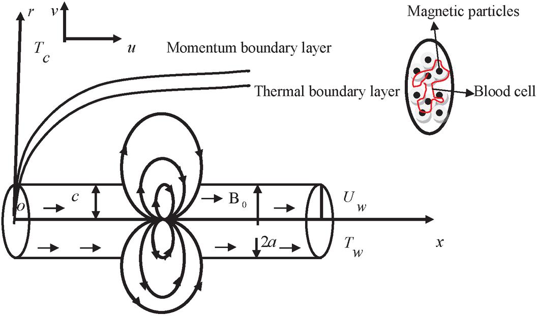
Figure 1 Schematic diagram of flow problem.

Under the above considerations we extend the idea of [30–32, 41] and here the continuity, momentum and energy equations are in following form:

Continuity equation

$$\frac{\partial }{\partial x}(ru)+\frac{\partial }{\partial r}(rv)=0$$

(1)

Momentum equations

$u{\displaystyle \frac{\partial u}{\partial x}}+v{\displaystyle \frac{\partial u}{\partial r}}$	$=-{\displaystyle \frac{1}{{\rho }_{mf}}}{\displaystyle \frac{\partial p}{\partial x}}+{\displaystyle \frac{{\mu }_{mf}}{{\rho }_{mf}}}\left({\displaystyle \frac{1}{r}}{\displaystyle \frac{\partial u}{\partial r}}+{\displaystyle \frac{{\partial }^{2}u}{\partial r^2}}+{\displaystyle \frac{{\partial }^{2}u}{\partial x^2}}\right)$
	$\mathrm{\hspace{1em}}-{\displaystyle \frac{{\sigma }_{mf}}{{\rho }_{mf}}}{B}_0^{2}u+{\displaystyle \frac{1}{{\rho }_{mf}}}{\mu }_0{M}_1{\displaystyle \frac{\partial H}{\partial x}}$	(2)
$u{\displaystyle \frac{\partial v}{\partial x}}+v{\displaystyle \frac{\partial v}{\partial r}}$	$=-{\displaystyle \frac{1}{{\rho }_{mf}}}{\displaystyle \frac{\partial p}{\partial r}}+{\displaystyle \frac{{\mu }_{mf}}{{\rho }_{mf}}}\left({\displaystyle \frac{1}{r}}{\displaystyle \frac{\partial v}{\partial r}}+{\displaystyle \frac{{\partial }^{2}v}{\partial r^2}}+{\displaystyle \frac{{\partial }^{2}v}{\partial x^2}}-{\displaystyle \frac{v}{r^2}}\right)$	(3)

Energy equation

${(\rho C_p)}_{mf}\left(u{\displaystyle \frac{\partial T}{\partial x}}+v{\displaystyle \frac{\partial T}{\partial r}}\right)+{\mu }_{0}T{\displaystyle \frac{\partial M_1}{\partial T}}\left(u{\displaystyle \frac{\partial H}{\partial x}}+v{\displaystyle \frac{\partial H}{\partial r}}\right)$
$\mathrm{\hspace{1em}\hspace{1em}}={\kappa }_{mf}\left({\displaystyle \frac{1}{r}}{\displaystyle \frac{\partial T}{\partial r}}+{\displaystyle \frac{{\partial }^{2}T}{\partial r^2}}+{\displaystyle \frac{{\partial }^{2}T}{\partial x^2}}\right)$	(4)

With associated boundary conditions

$u=U_w={\displaystyle \frac{u_{0}x}{l}},v=0,T=T_w$		$\text{at}r=a$	(5)
$u\to 0,T\to T_c,P+{\displaystyle \frac{1}{2}}\rho q^2=\text{constant}$		$\text{at}r\to \mathrm{\infty }$	(6)

Where, $u$ and $v$ are the velocity component along $x$ and $r$ axis, respectively ($\overrightarrow{q}=(u,v)$). Also $P,\rho ,\mu ,\sigma ,{\mu }_0,{\mathrm{M}}_1,H,C_p,\kappa$ denotes the biomagnetic fluid pressure, density, dynamic viscosity, electrical conductivity, magnetic permeability, magnetization, magnetic field of strength, specific heat at constant pressure and thermal conductivity respectively. $B_0$ is the mean value of steady magnetic field of strength inside the flow field. The symbol ${()}_{mf}$, represents the magnetic fluid. In Equation (2), the term ${\mu }_0{M}_1\frac{\partial H_1}{\partial x}$ indicates the components of ferromagnetic body force per unit; while the term ${\mu }_{0}T\frac{\partial M_1}{\partial T}(u\frac{\partial H}{\partial x}+v\frac{\partial H}{\partial r})$ in Equation (4) accounts for heating due to adiabatic magnetization. These terms are well known as FHD. In Equation (2) the term $\frac{{\sigma }_{mf}}{{\rho }_{mf}}{B}_0^{2}u$ represents force per unit volume towards $x$-direction and arises due to the electrical conductivity of the fluid (blood). These term arise because of MHD.

Considering the studies of [23] and [32], the magnetic dipole gives rise to a magnetic field sufficiently strong to saturate the biofluid and its scalar potential is given by

$$V=\frac{\alpha }{2\pi }\frac{x}{x^2+{(r+c)}^2}$$

(7)

Here, $\alpha =\sqrt{\frac{u_0}{{\upsilon }_f}{c}^2}$ is a dimensionless distance and $\alpha =\gamma$ where$\gamma$ indicates the strength of magnetic field at the source position.

Therefore, the magnitude of the magnetic field of intensity i.e. $\parallel \overrightarrow{H}\parallel =H$ is given by

$$\parallel \overrightarrow{H}\parallel =H(x,r)=\sqrt{H_x^2+H_r^2}=\frac{\gamma }{2\pi }\frac{x^2}{x^2+{(r+c)}^2}$$

(8)

And $H_x,H_r$ are the components of the magnetic field $\overrightarrow{H}=(H_x,H_r)$ given by

$H_x(x,r)$	$=-{\displaystyle \frac{\partial V}{\partial x}}={\displaystyle \frac{\gamma }{2\pi }}{\displaystyle \frac{x^2-{(r+c)}^2}{{(x^2+{(r+c)}^2)}^2}}$	(9)
$H_r(x,r)$	$=-{\displaystyle \frac{\partial V}{\partial r}}={\displaystyle \frac{\gamma }{2\pi }}{\displaystyle \frac{2x(r+c)}{{(x^2+{(r+c)}^2)}^2}}$	(10)

After calculations of (9) and (10), the component takes the form

${\displaystyle \frac{\partial H}{\partial x}}$	$=-{\displaystyle \frac{\gamma }{2\pi }}{\displaystyle \frac{2x}{{(r+c)}^4}}$	(11)
${\displaystyle \frac{\partial H}{\partial r}}$	$=-{\displaystyle \frac{\gamma }{2\pi }}\left({\displaystyle \frac{-2}{{(r+c)}^3}}+{\displaystyle \frac{4x^2}{{(r+c)}^5}}\right)$	(12)

Thus, the magnetic field intensity $H$ can be expressed as

$$H(x,r)=\frac{\gamma }{2\pi }\left(\frac{1}{{(r+c)}^2}-\frac{x^2}{{(r+c)}^4}\right)$$

(13)

The variation of magnetization $M_1$ with temperature $T$ is defined by a linear relation [32]

$$M_1=K(T_c-T)$$

(14)

Where, $K$ represents the pyromagnetic coefficient and $T_c$ is the Curie temperature.

The thermo-physical factors of magnetic particles are defined as [30]

${\mu }_{mf}$	$={\mu }_f{(1-\varphi )}^{-2.5},{(\rho C_p)}_{mf}=(1-\varphi ){(\rho C_p)}_f+\varphi {(\rho C_p)}_s,$
${\rho }_{mf}$	$=(1-\varphi ){\rho }_f+\varphi {\rho }_s,$
${\sigma }_{mf}$	$=(1-\varphi ){\sigma }_f+\varphi {\sigma }_s,{\displaystyle \frac{{\kappa }_{mf}}{{\kappa }_f}}={\displaystyle \frac{({\kappa }_s+2{\kappa }_f)-2\varphi ({\kappa }_f-{\kappa }_s)}{({\kappa }_s+2{\kappa }_f)+\varphi ({\kappa }_f-{\kappa }_s)}}$	(15)

Here, $\varphi$ indicates the volume fraction where, $\varphi =0$ corresponds to regular fluid. Note that ${()}_f$ and ${()}_s$ signifies the base fluid (blood) and magnetic particles (Fe${}_3$O${}_4$).

Solution Procedure

For the implementation of the numerical solution we introduce the similarity transformation in order to make the momentum and energy equations dimensionless [32]

$$\begin{array}{c}\eta (r)=\frac{r^2-a^2}{2a}{\left(\frac{U_w}{{\upsilon }_{f}x}\right)}^{\frac{1}{2}}=\frac{r^2-a^2}{2a}{\left(\frac{u_0}{{\upsilon }_{f}l}\right)}^{\frac{1}{2}}\hfill \\ \xi \left(x\right)={\left(\frac{u_0}{{\upsilon }_{f}l}\right)}^{\frac{1}{2}}x,\psi (\xi ,\eta )={\left(\frac{u_0{\upsilon }_f}{l}\right)}^{\frac{1}{2}}axf(\eta )\hfill \\ \theta (\xi ,\eta )=\frac{T_c-T}{T_c-T_w}={\theta }_1(\eta )+{\xi }^2{\theta }_2(\eta )\hfill \\ P(\xi ,\eta )=\frac{P}{\frac{u_0{\mu }_f}{l}}=-[P_1(\eta )+{\xi }^2{P}_2(\eta )]\hfill \end{array}\}$$

(16)

Where, $\psi (\xi ,\eta ),\theta (\xi ,\eta )$ and $P(\xi ,\eta )$ are the stream function, the dimensionless temperature and pressure respectively. The continuity equation is satisfied considering the velocity components as follows

$$\{\begin{array}{c}u=\frac{1}{r}\frac{\partial \psi }{\partial r}\hfill \\ v=-\frac{1}{r}\frac{\partial \psi }{\partial x}\hfill \end{array}$$

(17)

We substitute Equations (11) to (17) into Equations (2) to (4) and then equating the coefficients of equal power of $\xi$ up to${\xi }^2$, we get

$(1+2\eta D)f^{\prime \prime \prime }+2D{f}^{\prime \prime }-{(1-\varphi )}^{2.5}\left(1-\varphi +\varphi {\displaystyle \frac{{\sigma }_s}{{\sigma }_f}}\right)M{f}^{\prime }$
$\mathrm{\hspace{1em}\hspace{1em}}-{\left(1-\varphi \right)}^{2.5}\left(1-\varphi +\varphi {\displaystyle \frac{{\rho }_s}{{\rho }_f}}\right)(f^{\prime 2}-f{f}^{\prime \prime })$
$\mathrm{\hspace{1em}\hspace{1em}}+2{(1-\varphi )}^{2.5}{P}_2-{(1-\varphi )}^{2.5}{\displaystyle \frac{2\beta {\theta }_1}{{(\eta +\alpha )}^4}}=0$	(18)
${(1+2\eta D)}^2{(1-\varphi )}^{2.5}{P}_1^{\prime }-{(1+2\eta D)}^2{f}^{\prime \prime }$
$\mathrm{\hspace{1em}\hspace{1em}}+{(1-\varphi )}^{2.5}\left(1-\varphi +\varphi {\displaystyle \frac{{\rho }_s}{{\rho }_f}}\right)(D{f}^2-(1+2\eta D)f{f}^{\prime })=0$	(19)
${(1+2\eta D)}^2{(1-\varphi )}^{2.5}{P}_2^{\prime }=0$	(20)
$(1+2\eta D){\theta }_1^{\prime \prime }+2{\theta }_2+2D{\theta }_1^{\prime }$
$\mathrm{\hspace{1em}\hspace{1em}}+{\displaystyle \frac{{\kappa }_f}{{\kappa }_{mf}}}\left(\left(1-\varphi +\varphi {\displaystyle \frac{{\left(\rho C_p\right)}_s}{{\left(\rho C_p\right)}_f}}\right)\mathrm{Pr}f{\theta }_1^{\prime }+{\displaystyle \frac{2\beta \lambda f({\theta }_1-\epsilon )}{{\left(\eta +\alpha \right)}^3}}\right)=0$
$(1+2\eta D){\theta }_2^{\prime \prime }+2D{\theta }_2^{\prime }$
$\mathrm{\hspace{1em}\hspace{1em}}+{\displaystyle \frac{{\kappa }_f}{{\kappa }_{mf}}}\left(\begin{array}{c}\left(1-\varphi +\varphi {\displaystyle \frac{{\left(\rho C_p\right)}_s}{{\left(\rho C_p\right)}_f}}\right)\mathrm{Pr}\left(f{\theta }_2^{\prime }-2f^{\prime }{\theta }_2\right)\hfill \\ -2\beta \lambda ({\theta }_1-\epsilon )\left[{\displaystyle \frac{f^{\prime }}{{\left(\eta +\alpha \right)}^4}}+{\displaystyle \frac{2f}{{\left(\eta +\alpha \right)}^5}}\right]+{\displaystyle \frac{2\beta \lambda f{\theta }_2}{{(\eta +\alpha )}^3}}\hfill \end{array}\right)=0$	(22)

And the boundary conditions (5) and (6) take the following form

$f=0,f^{\prime }=1,{\theta }_1=1,{\theta }_2=0$		$\text{at}\eta =0$	(23)
$f^{\prime }\to 0,{\theta }_1\to 0,{\theta }_2\to 0,P_1\to -P_{\mathrm{\infty }},P_2\to 0$		$\text{at}\eta \to \mathrm{\infty }$	(24)

Here the dimensionless parameters that appear in the above equations are defined as

Ferromagnetic interaction parameter $\beta =\frac{\gamma }{2\pi }\frac{{\mu }_{0}K(T_c-T_w){\rho }_f}{{\mu }_f^2}$; Magnetic field parameter $M=\frac{{\sigma }_f{B}_0^{2}l}{u_0{\rho }_f}$; viscous dissipation parameter $\lambda =\frac{u_0{\mu }_f^2}{l{k}_f(T_c-T_w){\rho }_f}$; Curie temperature $\epsilon =\frac{T_c}{T_c-T_w}$; Curvature parameter $D={(\frac{l{\upsilon }_f}{u_0{a}^2})}^{\frac{1}{2}}$; Dimensionless distance $\alpha ={(\frac{u_0}{{\upsilon }_f})}^{\frac{1}{2}}c$; Prandtl number $\mathrm{Pr}=\frac{{(\mu C_p)}_f}{{\kappa }_f}$.

Numerical Technique

In this section we describe the numerical solution of the problem where we apply an approximate technique that has better stability characteristics than a classical Runge-Kutta combined with a shooting method, is simple, accurate and efficient. The detail study of this technique can be found in [14, 40]. The most important features of this technique are:

(1) It is based on the common finite difference method with central differencing.

(2) On a tridiagonal matrix manipulation, and

(3) On an iterative procedure

According [14, 40], we can write the momentum Equation (19) is following way:

$(1+2\eta D)f^{\prime \prime \prime }+2D{f}^{\prime \prime }-{(1-\varphi )}^{2.5}$

$\mathrm{\hspace{1em}\hspace{1em}}\left((1-\varphi +\varphi {\displaystyle \frac{{\sigma }_s}{{\sigma }_f}})M{f}^{\prime }+\left(1-\varphi +\varphi {\displaystyle \frac{{\rho }_s}{{\rho }_f}}\right)f^{\prime 2}\right)+{(1-\varphi )}^{2.5}$

$\mathrm{\hspace{1em}\hspace{1em}}\left(1-\varphi +\varphi {\displaystyle \frac{{\rho }_s}{{\rho }_f}}\right)f{f}^{\prime \prime }={(1-\varphi )}^{2.5}{\displaystyle \frac{2\beta {\theta }_1}{{(\eta +\alpha )}^4}}-2{(1-\varphi )}^{2.5}{P}_2$

By putting $y(x)=f^{\prime }(\eta )$, the Equation (25) can be considered as a second order linear differential equation and provided that $P_2$ and $f(\eta )$ are assumed to be known functions.

In this case Equation (25) can be written as

$(1+2\eta D){(f^{\prime })}^{\prime \prime }+\left(2D+{(1-\varphi )}^{2.5}\left(1-\varphi +\varphi {\displaystyle \frac{{\rho }_s}{{\rho }_f}}\right)f\right){(f^{\prime })}^{\prime }$

$\mathrm{\hspace{1em}\hspace{1em}}-\left({(1-\varphi )}^{2.5}\left(1-\varphi +\varphi {\displaystyle \frac{{\sigma }_s}{{\sigma }_f}}\right)M+{(1-\varphi )}^{2.5}\left(1-\varphi +\varphi {\displaystyle \frac{{\rho }_s}{{\rho }_f}}\right)f^{\prime }\right)$

$\mathrm{\hspace{1em}\hspace{1em}}{f}^{\prime }={(1-\varphi )}^{2.5}{\displaystyle \frac{2\beta {\theta }_1}{{(\eta +\alpha )}^4}}-2{(1-\varphi )}^{2.5}{P}_2$

Which takes the form

$$P(x)y^{\prime \prime }(x)+\mathrm{Q}(x)y^{\prime }(x)+\mathrm{R}(x)y(x)=\mathrm{S}(x)$$

(26)

Where,

$P(x)$	$=1+2\eta \mathrm{D},Q(x)=2D-{(1-\varphi )}^{2.5}\left(1-\varphi +\varphi {\displaystyle \frac{{\rho }_s}{{\rho }_f}}\right)f,$
$R(x)$	$=-{(1-\varphi )}^{2.5}\left(1-\varphi +\varphi {\displaystyle \frac{{\sigma }_s}{{\sigma }_f}}\right)M$
	$\mathrm{\hspace{1em}}-{(1-\varphi )}^{2.5}\left(1-\varphi +\varphi {\displaystyle \frac{{\rho }_s}{{\rho }_f}}\right)f^{\prime },$
$S(x)$	$={(1-\varphi )}^{2.5}{\displaystyle \frac{2\beta {\theta }_1}{{(\eta +\alpha )}^4}}-2{(1-\varphi )}^{2.5}{P}_2$

Now Equation (26) can be solved by a common finite difference method, based on central differencing and tridiagonal matrix manipulation, before starting solution procedure, it’s essential to give an initial guess for $f^{\prime }(\eta )$ and $P_2(\eta )$ between $\eta =0$ and $\eta ={\eta }_{\mathrm{\infty }}(\eta \to \mathrm{\infty })$ which satisfy the boundary conditions of (23) and (24). For this we assume as initial distributions that,

$$f^{\prime }(\eta )=1-\frac{\eta }{{\eta }_{\mathrm{\infty }}},{\theta }_1=1-\frac{\eta }{{\eta }_{\mathrm{\infty }}},{\theta }_2=\frac{1}{2}\left(\frac{\eta }{{\eta }_{\mathrm{\infty }}}\right)\left(1-\frac{\eta }{{\eta }_{\mathrm{\infty }}}\right)$$

The $f(\eta )$ distribution is obtained by the integration from $f^{\prime }(\eta )$ curve. The next step is to consider $f,P_2$ and ${\theta }_1$ known and to determine a new estimation for $f^{\prime }(\eta ),(f_{new}^{\prime })$ by solving the nonlinear Equation (26) using the above method. The $f(\eta )$ distribution is updated by integrating the new $f^{\prime }(\eta )$ curves. These new profiles $f$ and $f^{\prime }$ are then used to new inputs and so on. In this way the momentum Equation (25) and consequently (18) are solved iteratively until convergence up to a small quantity ${\epsilon }_1$ is attained.

Following the same algorithm, Equations (21) and (22) with boundary conditions (23) and (24) are solved after $f(\eta )$ is obtained.

Now energy Equations (21) and (22) can be written in the form of Equation (26) that is

$(1+2\eta D){\theta }_1^{\prime \prime }+\left(2D+{\displaystyle \frac{{\kappa }_f}{{\kappa }_{mf}}}\left(1-\varphi +\varphi {\displaystyle \frac{{(\rho C_p)}_s}{{(\rho C_p)}_f}}\right)\mathrm{Pr}f\right){\theta }_1^{\prime }$
$\mathrm{\hspace{1em}\hspace{1em}}-{\displaystyle \frac{{\kappa }_f}{{\kappa }_{mf}}}{\displaystyle \frac{2\beta \lambda f}{{(\eta +\alpha )}^3}}{\theta }_1={\displaystyle \frac{{\kappa }_f}{{\kappa }_{mf}}}{\displaystyle \frac{2\beta \lambda f\epsilon }{{(\eta +\alpha )}^3}}-2{\theta }_2$	(27)

By setting $y(x)={\theta }_1(\eta )$ in Equation (28), we get

$$P(x)y^{\prime \prime }(x)+\mathrm{Q}(x)y^{\prime }(x)+\mathrm{R}(x)y(x)=\mathrm{S}(x)$$

(28)

Where,

$P(x)$	$=1+2\eta \mathrm{D},Q(x)$
	$=2D+{\displaystyle \frac{{\kappa }_f}{{\kappa }_{mf}}}\left(1-\varphi +\varphi {\displaystyle \frac{{(\rho C_p)}_s}{{(\rho C_p)}_f}}\right)\mathrm{Pr}f,$
$R(x)$	$=-{\displaystyle \frac{{\kappa }_f}{{\kappa }_{mf}}}{\displaystyle \frac{2\beta \lambda f}{{(\eta +\alpha )}^3}},$
$S(x)$	$={\displaystyle \frac{{\kappa }_f}{{\kappa }_{mf}}}{\displaystyle \frac{2\beta \lambda f\epsilon }{{(\eta +\alpha )}^3}}-2{\theta }_2$

Similarly Equation (23) can be written as

$(1+2\eta D){\theta }_2^{\prime \prime }+\left(2D+{\displaystyle \frac{{\kappa }_f}{{\kappa }_{mf}}}\left(1-\varphi +\varphi {\displaystyle \frac{{(\rho C_p)}_s}{{(\rho C_p)}_f}}\right)\mathrm{Pr}f\right){\theta }_2^{\prime }$
$\mathrm{\hspace{1em}\hspace{1em}}+{\displaystyle \frac{{\kappa }_f}{{\kappa }_{mf}}}\left({\displaystyle \frac{2\beta \lambda f{\theta }_2}{{(\eta +\alpha )}^3}}-\left(1-\varphi +\varphi {\displaystyle \frac{{(\rho C_p)}_s}{{(\rho C_p)}_f}}\right)2\mathrm{P}\mathrm{r}{f}^{\prime }\right){\theta }_2$
$\mathrm{\hspace{1em}\hspace{1em}}={\displaystyle \frac{{\kappa }_f}{{\kappa }_{mf}}}2\beta \lambda ({\theta }_1-\epsilon )\left[{\displaystyle \frac{f^{\prime }}{{(\eta +\alpha )}^4}}+{\displaystyle \frac{2f}{{(\eta +\alpha )}^5}}\right]$	(29)

Again setting $y(x)={\theta }_2(\eta )$, Equation (30) are reduced in a second order differential equation and of the following form

$$P(x)y^{\prime \prime }(x)+\mathrm{Q}(x)y^{\prime }(x)+\mathrm{R}(x)y(x)=\mathrm{S}(x)$$

(30)

Where,

$P(x)$	$=1+2\eta \mathrm{D},Q(x)=2D+{\displaystyle \frac{{\kappa }_f}{{\kappa }_{mf}}}\left(1-\varphi +\varphi {\displaystyle \frac{{(\rho C_p)}_s}{{(\rho C_p)}_f}}\right)\mathrm{Pr}f,$
$R(x)$	$={\displaystyle \frac{{\kappa }_f}{{\kappa }_{mf}}}\left({\displaystyle \frac{2\beta \lambda f{\theta }_2}{{(\eta +\alpha )}^3}}-\left(1-\varphi +\varphi {\displaystyle \frac{{(\rho C_p)}_s}{{(\rho C_p)}_f}}\right)2\mathrm{P}\mathrm{r}{f}^{\prime }\right),$
$S(x)$	$={\displaystyle \frac{{\kappa }_f}{{\kappa }_{mf}}}2\beta \lambda ({\theta }_1-\epsilon )\left[{\displaystyle \frac{f^{\prime }}{{(\eta +\alpha )}^4}}+{\displaystyle \frac{2f}{{(\eta +\alpha )}^5}}\right]$

In this way we obtain ${\theta }_1$ and ${\theta }_2$ until the convergence up to a small quantity ${\epsilon }_1$ is attained. Then now we obtain new estimates of $P_1$ and $P_2$ from Equations (19) and (20), respectively, which are already first order linear differential equation. This process is continuing until the trial convergence of the solution is attained. For the numerical solution we apply a step size $h=\mathrm{\Delta }\eta =0.01$, ${\eta }_{\min }=0$ and ${\eta }_{\max }=1$; and the solution is convergent with an approximation of ${10}^{-3}$.

Validation

Before proceeding to the numerical calculation, it’s necessary to check the accuracy of the numerical technique and for that we compared our present numerical results with those published in the study [32]. An indicative graphical representation of the comparison is given at Figures 2 and 3 where our results has been found in good agreement with those obtained in [32]. Furthermore, we also compared the rate of heat transfer for different values of Prandtl number Pr. These results are presented at Table 1 and also verify the good agreement with the results obtained in [32].

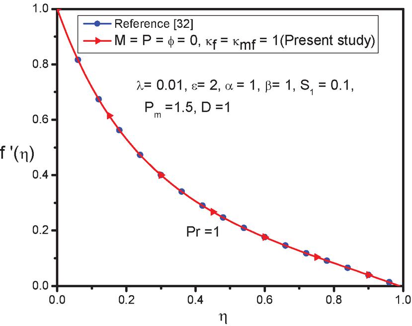
Figure 2 Comparison of velocity profile for $M=P=\varphi =0,{\kappa }_f={\kappa }_{mf}=1$.

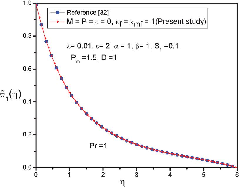
Figure 3 Comparison of Temperature profile for $M=P=\varphi =0,{\kappa }_f={\kappa }_{mf}=1$.

Results and Discussion

In this section we discuss the results presented graphically with respect of the effect of the dimensionless parameters for velocity, temperature, pressure, skin friction coefficient, rate of heat transfer and pressure gradient. In order to attain this, we need to put some realistic values which published previously and relative to this paper. So, we assume the fluid is blood and the magnetic particles are Fe${}_3$O${}_4$, and following the literature [19, 20, 33–36] we adopt the values of properties of blood and Fe${}_3$O${}_4$ given in Table 2.

Table 1 Comparison of the rate of heat transfer with [32] for various values of Pr when $M=P=\varphi =0,{\kappa }_f={\kappa }_{mf}=1$

Pr	Present Result	Tahir et al. [32]	$|Error|$
1	0.5131	0.5132769	0.0001769
1.3	0.5858	0.5982321	0.0182321
1.9	0.6324	0.6312902	0.0011098
4	0.8807	0.8892303	0.0085303
10	1.801	1.8002134	0.0007866

Table 2 Thermo-physical values of blood and Fe${}_3$O${}_4$

Physical Properties	$C_p(jk{g}^{-1}{K}^{-1})$	$\rho (kg{m}^{-3})$	$\sigma (s{m}^{-1})$	$\kappa (W{m}^{-1}{K}^{-1})$
Blood	$3.9\times {10}^3$	1050	0.8	0.5
Fe${}_3$O${}_4$	670	5180	$0.74\times {10}^6$	9.7

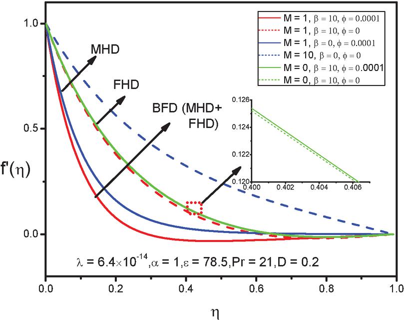
Figure 4 Axial velocity profile $f^{\prime }(\eta )$ for FHD, MHD and BFD.

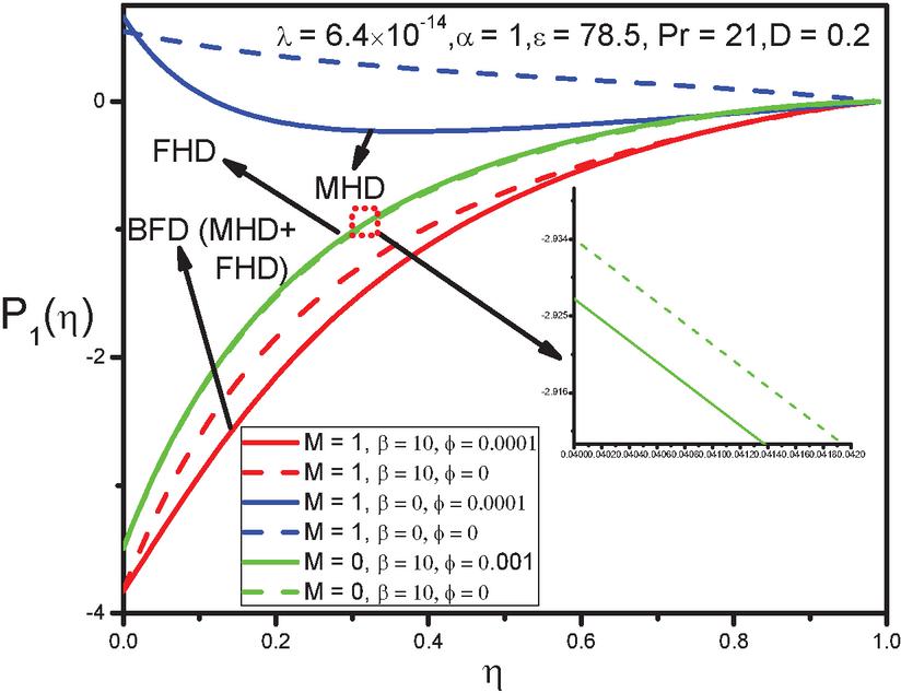
Figure 5 Pressure profile $P_1(\eta )$ for FHD, MHD and BFD.

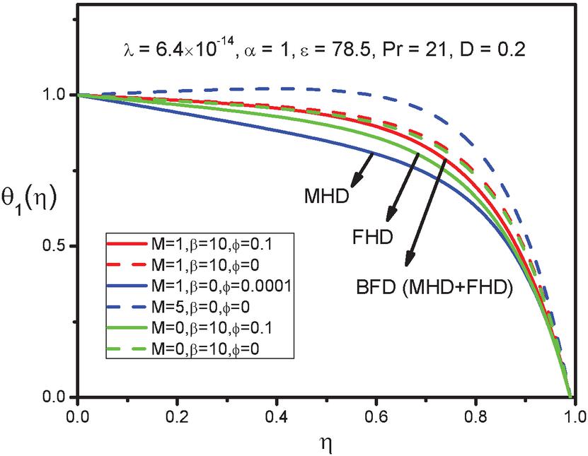
Figure 6 Temperature profile ${\theta }_1(\eta )$ for FHD, MHD and BFD.

Whereas human body temperature $T_w={37}^{\circ }$C [20], body Curie temperature is $T_c={41}^{\circ }$C. For above values dimensionless temperature $\epsilon =78.5$ [14], viscous dissipation number $\lambda =6.4\times {10}^{-14}$ [14] and dimensionless distance $\alpha =1$ [19]. For numerical calculation the values of leading parameters Prandtl number $\mathrm{Pr}=17,21,23,25$ [19], magnetic parameter $M=0.1,0.5,0.5,0.7,1,5,10$ [37, 38], volume fraction $\varphi =0.0,0.0001,0.001,0.005,0.1,0.15,0.2$ [39], curvature parameter $D=0.1,0.2,0.5,1,1.5,2$ [31, 32] and ferromagnetic interaction parameter $\beta =0,5,10$ [14]. Note down when $M=0,\beta \ne 0$ indicates to pure ferrohydrodynamic flow (FHD), $M\ne 0,\beta =0$ indicates to pure magnetohydrodynamic flow (MHD) and $M\ne 0,\beta \ne 0$ indicates to mixed FHD and MHD flow which appears in the biomagnetic fluid flow (BFD) [13].

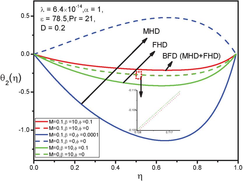
Figure 7 Temperature profile ${\theta }_2(\eta )$ for FHD, MHD and BFD.

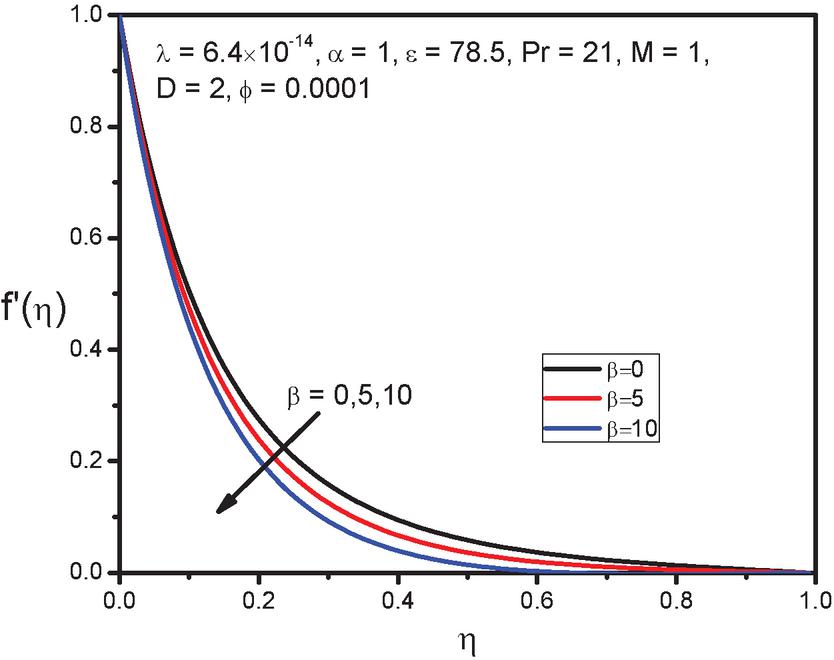
Figure 8 Influence of $\beta$ on axial velocity profile $f^{\prime }(\eta )$.

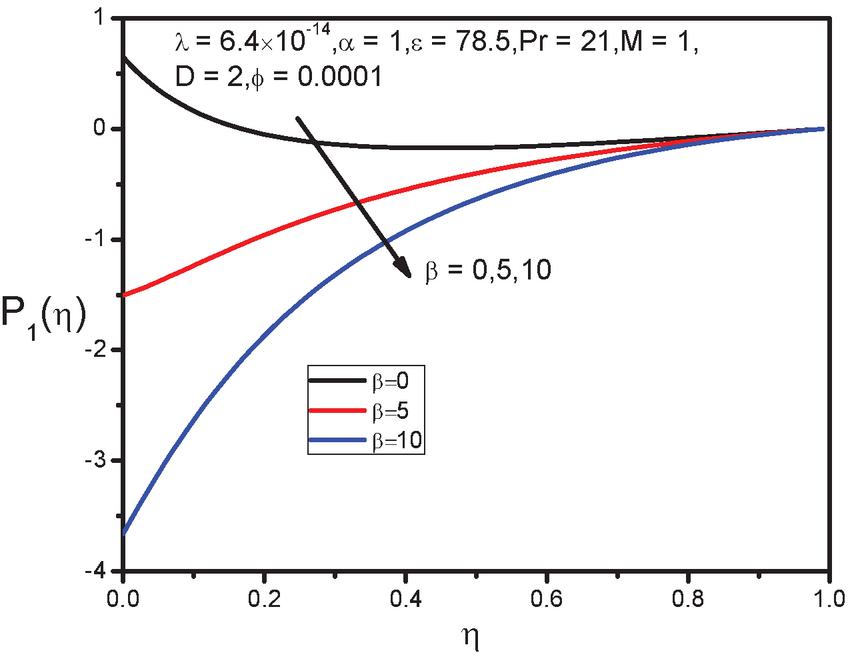
Figure 9 Influence of $\beta$ on pressure profile $P_1(\eta )$.

Figure 10 Influence of $\beta$ on temperature profile ${\theta }_1(\eta )$.

Figure 11 Influence of $\beta$ on temperature profile ${\theta }_2(\eta )$.

The influence of magnetic particles volume fraction on FHD, MHD and BFD in axial velocity, pressure and temperature profile can be observed from Figures 4 to 7. Where Figure 4 indicate that the decrement of the axial velocity for BFD is greater than FHD and MHD. It also clears that when we added magnetic particles with base fluid like blood, the decrement of BFD is more pronounced than pure BFD fluid. From the pressure profile (see Figure 5) we see that in case of BFD pressure is more comfortable to control rather than FHD and MHD. On the other hand, from the temperature profiles (see Figures 6 and 7) we observed that in case of BFD, temperature is increased much better than FHD and MHD cases under the influence of magnetic particles. Moreover, in the absence of magnetic particles, MHD is increased much effectively than BFD and FHD cases.

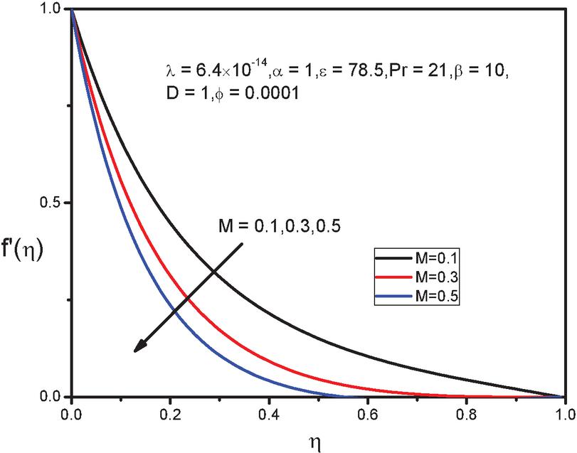
Figure 12 Influence of $M$ on axial velocity profile $f^{\prime }(\eta )$.

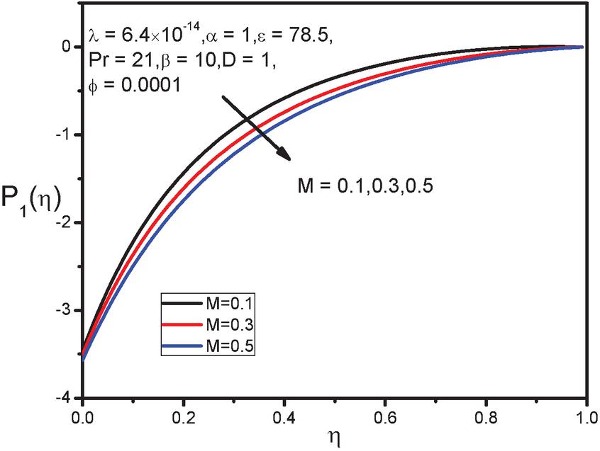
Figure 13 Influence of $M$ on pressure profile $P_1(\eta )$.

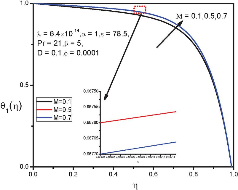
Figure 14 Influence of $M$ on temperature profile ${\theta }_1(\eta )$.

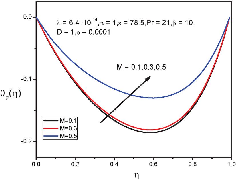
Figure 15 Influence of $M$ on temperature profile ${\theta }_2(\eta )$.

Figures 8 to 11 demonstrate the effect of ferromagnetic number on the axial velocity, pressure and temperature profile. From the pressure profile it is evident that as $\beta$ increases $P_1(\eta )$ is effectively reduced in the ferrohydrodynamic case especially for small values of $\eta$. Figures 10 to 11 show that the temperature profiles (see Figures 10 and 11) increase with raising values of $\beta$ and its augment noticed when $\beta >0$. The axial velocity $f^{\prime }(\eta )$ is reduced with increment of the values of ferromagnetic number (see Figure 8). This is happening due to the fact that $\beta$ is directly related to the Kelvin force.

Figures 12 to 15 present the variations of magnetic parameter on velocity, pressure and temperature distributions, respectively. It is apparent from Figure 12 that as magnetic parameter is increased, the axial velocity is reduced due to the fact that the presence of magnetic field produce Lorentz forces that act oppose to the flow. As the velocity is suppressed it is normal to see increment of the pressure profile as the values of $M$ are enhanced. The reverse behavior can be seen for the temperature profiles (see Figures 14 and 15).

Figures 16 to 19 portray the effect of various values of curvature parameter on velocity, pressure and temperature distributions, respectively. From Figure 16 it is observed that $f^{\prime }(\eta )$ increases as curvature is enhanced. This can be explained because when $D$ is increased the radius of cylinder decreases. As a result less resistance is provided on the surface which tumid the fluid velocity in boundary layer region. It discernible from Figures 18 and 19 that temperature profile ${\theta }_1(\eta )$ is reduced for higher values of curvature parameter but ${\theta }_2(\eta )$ is enhanced. With increasing values of $D$ we see that pressure profile $P_1(\eta )$ is also increased effectively (Figure 17).

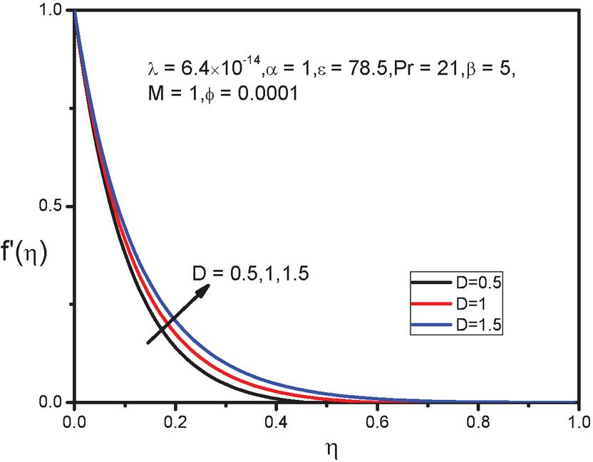
Figure 16 Influence of $D$ on axial velocity profile $f^{\prime }(\eta )$.

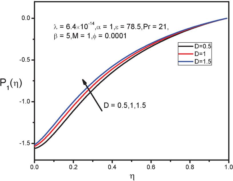
Figure 17 Influence of $D$ on pressure profile $P_1(\eta )$.

Figure 18 Influence of $D$ on temperature profile ${\theta }_1(\eta )$.

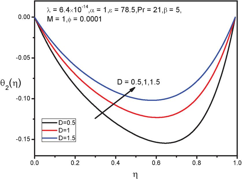
Figure 19 Influence of $D$ on temperature profile ${\theta }_2(\eta )$.

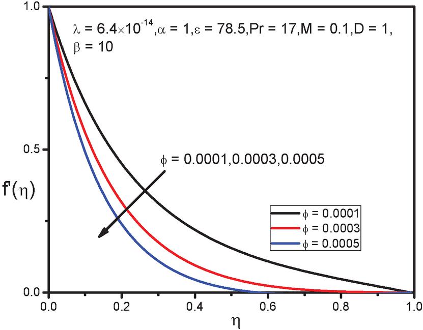
Figure 20 Influence of $\varphi$ on axial velocity profile $f^{\prime }(\eta )$.

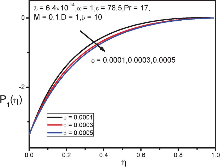
Figure 21 Influence of $\varphi$ on pressure profile $P_1(\eta )$.

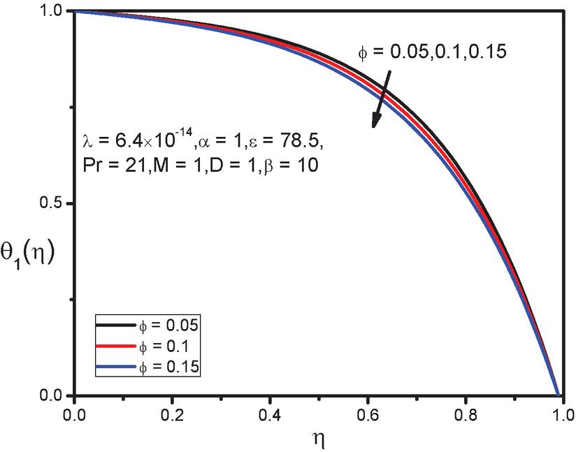
Figure 22 Influence of $\varphi$ on temperature profile ${\theta }_1(\eta )$.

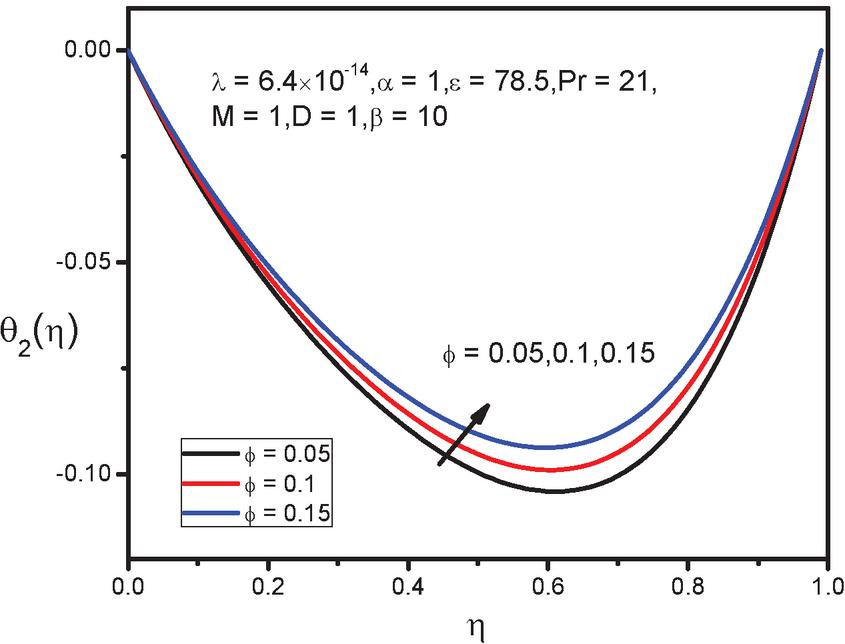
Figure 23 Influence of $\varphi$ on temperature profile ${\theta }_2(\eta )$.

Figures 20 to 23 plotted to observe the impact of magnetic particles volume fraction on velocity, temperature and pressure distributions, respectively. The fluid velocity $f^{\prime }(\eta )$ decreases with increasing values of volume fraction $\varphi$. This is due to the fact that magnetic particles spawn friction in fluids that creates a resistance to the flow. Since magnetic particles in large surface area produced high thermal conductivity, as a result thermal boundary layer is increased which is clearly visible in Figure 23 for the temperature profile ${\theta }_1(\eta )$ whereas the opposite is observed at Figure 22 which pictures the profile of the other temperature component ${\theta }_2(\eta )$. The pressure profile is gradually decreased with increasing values of volume fraction.

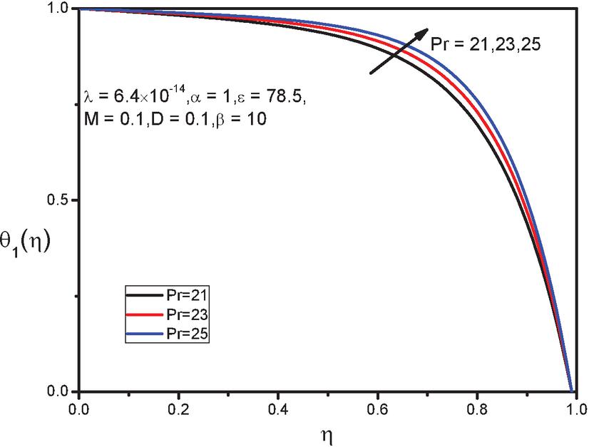
Figure 24 Influence of Pr on temperature profile ${\theta }_1(\eta )$.

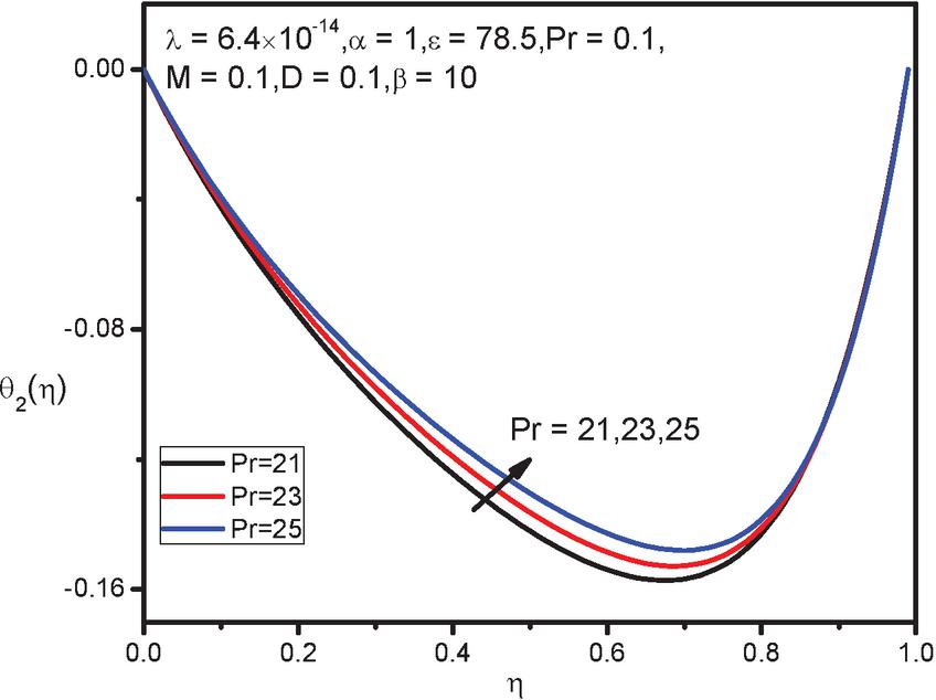
Figure 25 Influence of Pr on temperature profile ${\theta }_2(\eta )$.

Finally, Figures 24 and 25 represent the effect of the Prandtl number on temperature distributions. From Figures 24 and 25 it’s clearly seen that with increasing values of the Prandtl number temperature profiles ${\theta }_1(\eta )$ and ${\theta }_2(\eta )$ are reduced. Since Prandtl number is the ratio of momentum to thermal diffusion in boundary layer region.

One other interesting part of the study in engineer view is to graphically represent the skin friction coefficient, rate of heat transfer coefficient and wall pressure gradient. Mathematically, skin friction coefficient and rate of heat transfer coefficient are defined as

$$\begin{array}{c}{C}_f=-\frac{2{\tau }_{\mathrm{w}}}{{\rho }_f{U}_w^2}\hfill \\ N{u}_x=-\frac{x}{(T_c-T_w)}{\left(\frac{\partial \mathrm{T}}{\partial r}\right)}_{r=a}\hfill \end{array}\}$$

(31)

Where, ${\tau }_w={\mu }_{mf}{(\frac{\partial \mathrm{u}}{\partial r})}_{r=a}$ is the wall shear stress, using (16) and (17), Equation (31) reduces into

$C_f$	$=-{\displaystyle \frac{2}{{(1-\varphi )}^{2.5}}}{\mathrm{Re}}^{-\frac{1}{2}}{f}^{\prime \prime }(0)$	(32)
$N{u}_x$	$=-({\theta }_1^{\prime }(0)+{\xi }^2{\theta }_2^{\prime }(0)){\mathrm{Re}}^{\frac{1}{2}}$	(33)

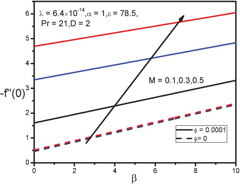
Figure 26 Skin friction coefficient $-f^{\prime \prime }(0)$ with $\beta$ for various values of$M$.

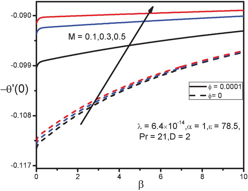
Figure 27 Rate of heat transfer $-{\theta }^{\prime }(0)$ with $\beta$ for various values of $M$.

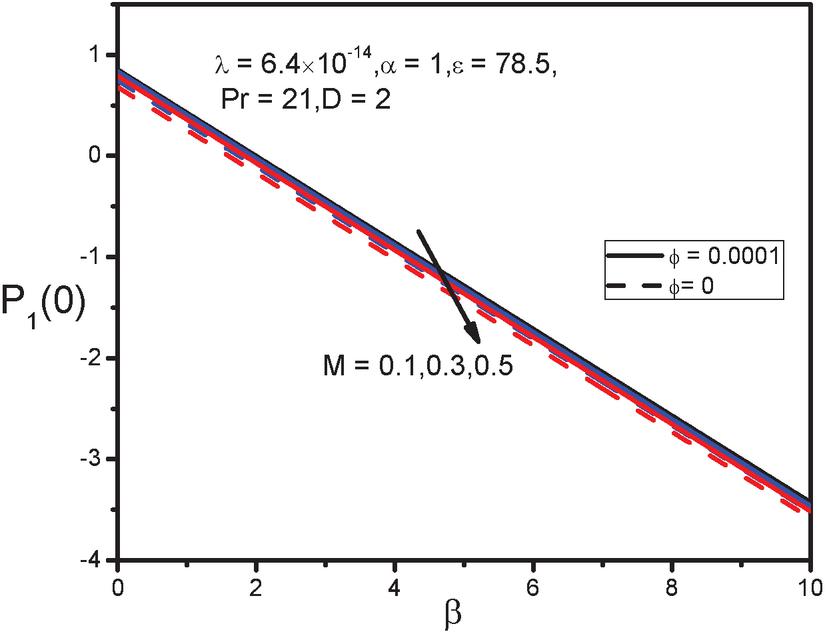
Figure 28 Wall pressure $P_1(0)$ with $\beta$ for various values of $M$.

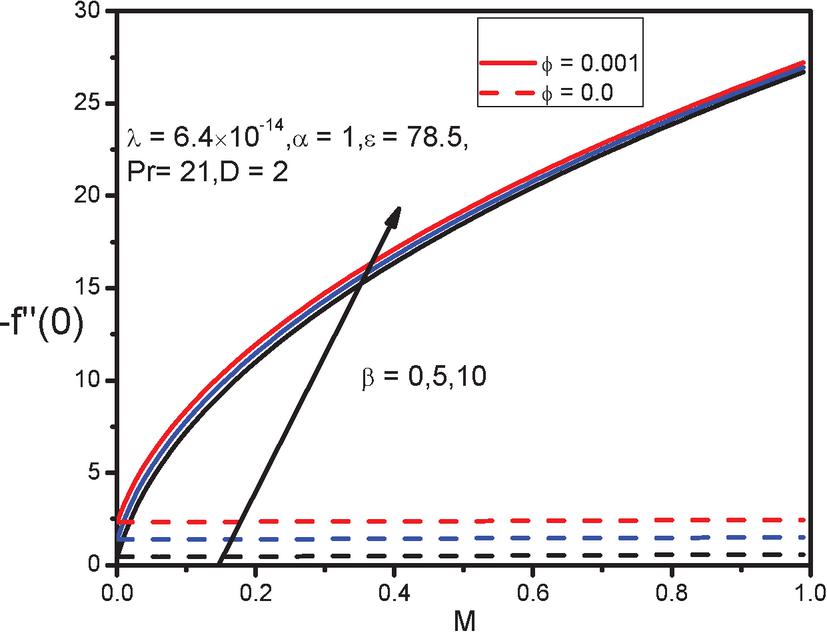
Figure 29 Skin friction coefficient $-f^{\prime \prime }(0)$ with $M$ for various values of $\beta$.

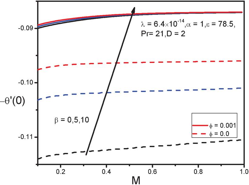
Figure 30 Rate of heat transfer $-{\theta }^{\prime }(0)$ with $M$ for various values of $\beta$.

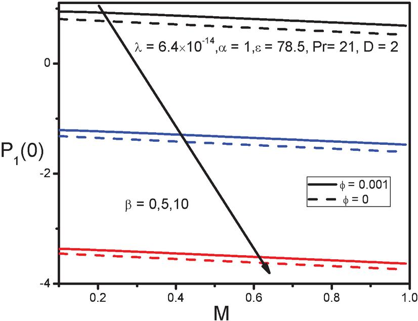
Figure 31 Wall pressure $P_1(0)$ with $M$ for various values of $\beta$.

Here $\mathrm{Re}=\frac{u_0{x}^2}{{\upsilon }_{f}l}$ known as local Reynolds number, $f^{\prime \prime }(0)$ and ${\theta }^{\prime }(0)=({\theta }_1^{\prime }(0)+{\xi }^2{\theta }_2^{\prime }(0))$ are defined as wall shear and wall heat transfer parameter, respectively.

Figures 26 to 31 demonstrate the skin friction coefficient, rate of heat transfer and wall pressure with $M$ and $\beta$ in the presence or absence of magnetic particles volume fraction, respectively. Where $P_1(0)$ represent the wall pressure parameter, solid line indicates when $\varphi \ne 0$ and dash line signifies when $\varphi =0$. From the Figures 26 to 31 it is apparent that $f^{\prime \prime }(0)$, ${\theta }^{\prime }(0)$ increase when values of $M$ and $\beta$ are enhanced respectively, whereas $P_1(0)$ is decreased. It also noticed from these figures that $f^{\prime \prime }(0)$ and ${\theta }^{\prime }(0)$ are always seems to be positive and negative, respectively throughout all their variation.

Conclusion

The main objective of the present study is to analyze the magnetic field effect on a base fluid like blood which is electrically conducting, contains magnetic particles and flows above a two-dimensional stretched cylinder in the presence of magnetic dipole. The numerical solution of the given problem carried out with the help of a finite differences method, based on central differencing, tridiagonal matrix manipulation and an iterative procedure. The effects of leading parameters which are involved with this model are studied and represented graphically. Such kind of problems is interesting in biomedicine. From the above analysis the basic conclusions are:

(1) After adding magnetic particles on blood, its flow is reduced, and the temperature is increased significantly using the extended BFD formulation comparatively to that of FHD or MHD.

(2) The axial velocity is decreased with increasing the values of the ferromagnetic number, magnetic parameter, and volume fraction whereas, is enhanced for large values of the curvature parameter.

(3) For enlarging values of the ferromagnetic number, magnetic parameter and Prandtl number the temperature profiles are enhanced.

(4) Opposite influence is observed in temperature profiles for curvature parameter and volume fraction.

(5) The pressure profile is decreased significantly with enhancing values of the ferromagnetic number, magnetic parameter and volume friction. The reverse behavior is obtained with the variation of the curvature parameter.

(6) For raising values of ferromagnetic number and magnetic parameter, skin friction coefficient and rate of heat transfer are increased respectively.

(7) The wall pressure is reduced for higher values of ferromagnetic number and magnetic parameter.

References

[1] Stark, D.D., Weissleder, R., Elizondo, G., Hahn, P.F., Saini, S., Todd, L.E., Wittenberg, J. and Ferucci, J.T. (1988). Superparamagnetic iron oxide: clinical application as a contrast for MR imaging of the liver, Radiology, 168: 297–301.

[2] Lu, J., Ma, S., Sun, J., Xia, C., Liu, C., Wang, Z. (2009). Magnetese ferrite nanoparticle micellarnanocomposites as MRI contrast agent for liver imaging, Biomaterials, 30:2919–2928.

[3] Suzuki, M., Honda, H., Kobayashi, T., Wakabayashi, T., Yoshida, J., and Takahashi, M. (1997). Development of a target directed magnetic resonance contrast agent using monoclonal antibody-conjugated magnetic particles, Brain Tumor Pathol, 13: 127–132.

[4] Durr, S., Janko, C., Lyer, S., Tripal, p., Schwarz, M., Zaloga, J., Toetze, R. and Alexiou, C. (2013). Magnetic nanoparticles for cancer therapy. Nanotechnol Rev. 2(4): 395–409.

[5] Jordan, A., Scholz, R., Wust, P., Fahling, H. and Felix, R. (1999). Magnetic fluid hyperthermia(MCFH): Cancer treatment with AC magnetic field induced excitation of biocompatible superparamagnetic nanoparticles, J. Magn. Magn. Mater., 201: 413–9.

[6] Mah, C., Zolotukhin, I., Fraites, T.J., Dobson, J., Batich, C. and Byrne, B.J. (2000). Micro-sphere mediated delivery of recombinant: AAV vectors in vitro and in vivo. Mol Therapy, 1:S239.

[7] Panatarotto, D., Prtidos, C.D., Hoebeke, J., Brown, F., Karmer, E., Briand, J.P., Muller, S., Prato, M. and Bianco, A. (2003). Immunization with peptide-functionalized carbon nanotubes enhances virus-specific neutralizing antibody responses. Chemistry & Biology, 10: 961–966.

[8] Joubert, J.C. and Quim, A.N. (1997). Magnetic microcomposites as vectors for bioactive agents, The state of Art. Intd. Ed.: 93S70.

[9] Goodwin, S. (2000). Magnetic targeted carries offer site-specific drug delivery. Oncol News Int, 9:22

[10] Dubertret, B., Skourides, P., Norris, D.J., Noireaux, V., Brivanlou, A.H. (2002). In vivo imaging of quantum dots encapsulated in phospholipids micelles, Science, 298(5599): 1759–1762.

[11] Gao, X.H., Cui, Y.Y., Levenson, R.M., Chung, L.W.K. and Nie, S.M. (2004). In vivo cancer targeting and imaging with semiconductor quantum dots. Nat Biotechnol, 22(8): 969–976.

[12] Haik,Y., Chen, J.C., Pai, V.M. (1996). Development of bio-magnetic fluid dynamics, in: S.H. Winoto, Y.T. Chew, N.E. Wijeysundera (Eds.),Proceedings of the IX International Symposium on Transport Properties in Thermal Fluids Engineering, Singapore, Pacific Center of Thermal Fluid Engineering, Hawaii, USA, 121–126.

[13] Tzirtzilakis, E.E. (2005). A mathematical model for blood flow in magnetic field, Phys. Fluids,17(7): 077103-1–14.

[14] Murtaza, M.G., Tzirtzilakis, E.E. and Ferdows, M. (2017). Effect of electrical conductivity and magnetization on the biomagnetic fluid flow over a stretching sheet, Zeitschrift fur angewandteMathematik und Physik, 68: 93.

[15] Misra, J.C. and Shit G.C. (2009). Biomagnetic viscoelastic fluid flow over a stretching sheet, Appl. Math. Comput., 210: 350.

[16] Murtaza, M.G., Ferdows, M., Tzirtzilakis, E.E. (2020). Stability and convergence analysis of a biomagnetic fluid flow over a stretching sheet in the presence of a magnetic field, Symmetry, 12:253.

[17] Murtaza, M.G., Ferdows, M., Tzirtzilakis, E.E., Misra, J.C. (2019). Three dimensional biomagnetic Maxwell fluid flow over a stretching surface in presence of heat source/sink, Internation Journal of Biomathematics, 12(3):12.

[18] Misra, J.C. and Shit G.C. (2009). Flow of a biomagnetic viscoelastic fluid in a channel with stretching walls, Journal of Applied Mechanics Trans. ASME, 76, 06106: 1–9.

[19] Tzirtzilakis, E.E. and Kafoussias, N. G. (2003). Biomagnetic fluid flow over a stretching sheet with nonlinear temperature dependent magnetization, Z. Angew. Math. Phys (ZAMP), 8:54–65.

[20] Tzirtzilakis, E.E., Xenos, M., Loukopoulos., V.C., Kafoussias, N.G. (2006). Turbulent biomagnetic fluid flow in a rectangular channel under the action of a localized magnetic field, International Journal of Engineering Science, 44(18–19), 1205–1224.

[21] Choi, SUS. (1995). Enhancing thermal conductivity of fluids with nanoparticles, in Proceedings of the ASME International Mechanical Engineering Congress and Exposition, San Francisco, CA, USA, 99–105.

[22] Misra, S. and Kamatam G. (2020). Effect of magnetic field, heat generation and absorption on nanofluid flow over a nonlinear stretching sheet, Journal of Nanotechnology, 11: 976–990.

[23] Neuringer, J.L. (1996). Some viscous flows of a saturated ferrofluid under the combined the influence of thermal and magnetic field gradients, Int. J. of Non-linear Mech., 1(2): 123–137.

[24] Elsayed, M. and Abd-Elaziz Mohamed, I.A. (2019). Effect of Thomson and thermal loading to laser pulse in a magneto-thermo elastic porous medium with energy dissipation, Z. Angew Math Mech (ZAMM), 99, e201900079.

[25] Sheikholeslami, M. and Ellahi, R. (2015). Electrohydrodynamicnanofluid hydrothermal treatment in an enclosure with sinusoidal upper wall, Appl. Sci., 5: 294–306.

[26] Rashidi, M.M. and Abelman, S. and FreidooniMehr, N. (2013). Entropy generation in steady MHD flow due to rotating porous disk in a nanofluid, Int. J. Heat and mass Transfer, 62: 515–525.

[27] Ishak, A. and Nazar, R. (2009). Laminar boundary flow along a stretching cylinder, Eur. J. Sci. Res., 36(1):22–29.

[28] Bachok, N. and Ishak, A. (2010). Flow and heat transfer over a stretching cylinder with prescribed heat flux, Malyasian Journal of Mathematical Sciences, 4: 159–169.

[29] Mukhopadhyay, S. (2013). MHD boundary layer slip flow along a stretching cylinder, Ain Shams Eng. J., 4: 317–324.

[30] Qasim, M., Khan, Z.H., Khan, W.A. and Ali shah I. (2014). MHD boundary layer slip flow and heat transfer of ferrofluid along a stretching cylinder with prescribed heat flux, PLos One, 9(1):e83930.

[31] Nadeem, S., Ullah, N., Khan, A.U. and Akbar, T. (2017). Effect of homogeneous-heterogeneous reactions on ferrofluid in the presence of magnetic dipole along a stretching cylinder, Results in Physics, 7: 3574–3582.

[32] Tahir, H., Khan, U., Din, A., Chu, Y.U. and Muhammad, N. (2020). Heat transfer in a ferromagnetic chemically reactive species, Journal of Thermophysics and Heat Transfer, doi: 10.2514/1.T6143.

[33] Tzirtzilakis, E.E. (2015). Biomagnetic fluid flow in an aneurysm using ferrohydrodynamics principles, Physics Fluids, 27:061902.

[34] Reddy, S.R.R., Reddy, P.B.A. (2018). Biomathematical analysis for the stagnation point flow over a nonlinear stretching surface with the second order velocity slip and Titanium alloy nanoparticle, Front. Heat Mass Transfer, 12.

[35] Tzirtzilakis, E.E. and Xenos, M.A. (2013). Biomagnetic fluid flow in a driven cavity, Meccanica, 48:187.

[36] Aziz, A., Jamshed, W., Ali, Y. and Shams, M. (2020). Heat transfer and entropy analysis of Maxwell Hybrid nanofluid including effects of inclined magnetic field joule heating and thermal radiation, Discrete and Continous Dynamical Systems series S, 13(10): 2667–2690.

[37] Liqat, A., Xiaomin, L., Bagh, A., Saima, M. and Sohaib, A. (2019). Finite element simulation of multi-slip effects on unsteady MHD bioconvectivemicropolarnanofluid flow over a sheet with solutal and thermal convective boundary conditions, Coatings, 9:842.

[38] Tzirtzilakis, E.E. and Tanoudis, G.B. (2003). Numerical study of biomagnetic fluid flow over a stretching sheet with heat transfer, Int. J. of Numerical Methods for Heat and Fluid Flow, 13: 830.

[39] Kuttan, B.A., Manjunathan, B., Jayanthi, B. and Gireesha, B.J. (2020). Performance of four different nanoparticles in boundary layer flow over a stretching sheet in porous medium driven by buoyancy force, Int. J. of Applied Mechanics and Engineering, 25(2): 1–10.

[40] Kafoussias, N.G. and Williams, E.W. (1993). An improved approximation technique to obtain numerical solution of a class of two point boundary value similarity problems in fluid mechanics, International Journal for Numerical Methods in Fluids, 17: 145–162.

[41] Tzirtzilakis, E.E., Loukopoulos., V.C. (2005). Biofluid flow in a channel under the action of a uniform localized magnetic field, Comput Mech., 36:360–374.

Biographies

Jahangir Alam received the bachelor’s and master’s degree in Mathematics from Comilla University, Bangladesh in 2017 and 2018, respectively. He is currently a philosophy of doctorate degree (Ph.D.) student at the Department of Applied Mathematics, University of Dhaka, Bangladesh. His research activities are focused on modeling and implementation of bio-fluid model with thermo-physical properties of nanoparticles and analysis their proper applications in relevant fields.

M. G. Murtaza received the bachelor’s degree in Mathematics from University of Dhaka in 2006, the master’s degree in Applied Mathematics from University of Dhaka in 2008, and the philosophy of doctorate degree (Ph.D.) in Applied Mathematics from University of Dhaka in 2020, respectively. Since 2020, he has been working as an Associate professor at the Department of Mathematics, Faculty of Science, Comilla University, Cumilla-3506, Bangladesh. His research focuses on the modeling, analysis and implementation of numerical simulation of fluid flow problems, and analysis their appropriate applications.

Efstratios Tzirtzilakis is professor at the Department of Mechanical Engineering, University of the Peloponnese, Greece. He has a degree in Mathematics, an MSc in Applied Mathematics, and a PhD in Biomagnetic Fluid Dynamics (BFD). His research field lies in Computational Fluid Mechanics and especially BFD, ferrofluid and MagnetoHydrodynamic flows. He has published in mathematical formulation of BFD flow problems, numerical methods for the solution of fluid mechanics problems, internal and boundary layer flows, analytic solutions and generally, in the research area of applied mathematics. He is author or co-author of more than 50 papers in international refereed journal with more than 1300 references from other researchers. He is member of the Editorial Board of the “Mathematical Problems in Engineering” International Journal (JSR IF 1.305) and “Mathematics” JSR IF 2.258. He is an expert in BFD flows and two of his publications were selected for the “Virtual Journal of Biological Physics Research”, where the papers published are reviewed for second time by a different editor and consider to constitute frontier research. He has also include in the database $<$$<$Data for Updated science-wide author database of standardized citation indicators $>$$>$, for the years 2020 and 2021 which includes the top 2% of the researchers worldwide with respect the number of citations in a specific area of research. In the past he has received scholarships from the Greek State Scholarship Foundation during his graduate and post-doctoral studies.

Mohammad Ferdows received his Ph.D. degrees from the Department of Mechanical Engineering, Tokyo Metropolitan University, Japan. He worked as a Postdoctoral Research Associate at several Institute/University and also worked as Professor and Visiting Professor in Louisiana Tech University, King Abdulaziz University, King Abdullah University of Science and Technology. Currently he is working as Professor at the Department of Applied Mathematics, University of Dhaka, Bangladesh. His research interests are in fluid mechanics, transport phenomena and biomedical flow phenomena.

European Journal of Computational Mechanics, Vol. 31_1, 1–40.
doi: 10.13052/ejcm2642-2085.3111
© 2022 River Publishers

Abstract

List of Symbols

Introduction

Mathematical Flow Model

Solution Procedure

Numerical Technique

Validation

Results and Discussion

Conclusion

References

Biographies