Approximated Fundamental Solutions Based on Levi Functions

R. Gallego and E. Puertas García*

Department of Structural Mechanics and Hydraulic Engineering,
School of Civil Engineering, University of Granada,
Fuentenueva Campus, Spain
E-mail: epuertas@ugr.es
*Corresponding Author

Received 05 March 2019; Accepted 10 May 2019;
Publication 05 August 2019

Abstract

Fundamental Solutions (FS) are useful for numerical methods, specifically in applications such as the Boundary Element Method (BEM) or the Method of Fundamental Solutions (MFS). Obtaining analytically the FS for a given problem is frequently unfeasible since it entails the solution of a complex system of differential equations. In this paper, a novel method for the computation of approximate FS based in enhanced Levi Function is presented. The first terms of the enhanced Levi Function are computed analytically by an iterative procedure until the residual is regular at the collocation point. The last step in the computation of the FS is completed approximating the residual by Modified Radial Base Functions that are particular solutions of the problem equations.

The method is applied to potential problems with variable coefficients, and validated comparing to available analytically computed Fundamental Solutions.

Keywords: Fundamental Solution, Levi Function, Functionally Graded Materials

1 Introduction

Fundamental Solutions are known for many Partial Differential Equations (PDEs) with constant coefficients [1, 2] which are of scientific and engineering interest. However, when the coefficients are variable with the position, the solution is not available in explicit form but for some special cases [3, 4].

Several techniques have been proposed to solve problems with variable coefficients by the Boundary Element Method or similar techniques, but lead to domain-boundary integral equations. The Dual Reciprocity Method was developed by [5]. In this method, a domain source term is approximated with a series of Radial Basis Functions and particular solutions are employed to transfer the domain integrals to the boundary.

The Radial Integration Method is a transformation technique that was implemented by [6]. This method transform domain integrals to the boundary in order to remove singularities. [7] developed this technique to solve elastic problems with nonlinearly varying material parameters.

The Analog Equation Method [8] was applied successfully [9] to solve elastostatic problems for materials with spatially varying properties.

The parametrix or Levi Function [10] is used as a substitute of a Fundamental Solution in order to reduce a boundary value problem into a system of boundary-domain integral equations [11–13].

Additionally, Radial Basis Functions (RBFs) have been applied to solve many problems in science and engineering [14]. RBFs are employed in the development of methods for solving partial differential equations and are used in some of the aforementioned papers [9, 15–19].

One important class of materials where the mathematical modeling leads to differential equations with variable coefficients is the so called Functionally Graded Materials (FGM). FGM are natural or artificial materials whose properties, composition and/or structure vary spatially in a controlled manner in order to optimize their behavior against spatially varying demands [20, 21]. FGMs have great potential applications but their modelization by BEM techniques is largely prevented due to the lack of suitable Fundamental Solution.

The goal of this paper is to prove the feasibility of obtaining the Fundamental Solution of differential operators with variable coefficients by combining Levi Functions and Radial Basis Functions. The technique is first developed theoretically for a general operator A(x) and applied to the heat transfer problem in a FGM for the purpose of validating the proposed methodology.

2 Definition of Problem

Let us consider a general linear partial differential operator A(x) of order n. Its Fundamental Solution is given by the solution U(x; y) of the system of equations

A(x)U(x; y) = $δ (x; y)$

where $δ (x; y)$ is the Direc’s Delta function applied at $x = y; x, y \in Ω \subset R^{n}$ are the “observation” and “collocation” point, respectively.

A Levi Function of the operator A(x) is any function $U_{L} (x; y)$ such that

A(x)UL(x; y) = $δ (x; y) + R (x; y)$

where R(x; y) is “smoother” than $δ (x; y)$ at $x = y$ ; $R (x; y)$ will be named “residual” of the Levi Function.

Defining,

UR(x; y) = U(x; y) - UL(x; y)

which is termed the “remainder”, is obvious that,

A(x)UR(x; y) = R(x; y)

The method for calculate the Fundamental Solution

$U (x; y)$ is divided in two steps: firstly a Levi Function $U_{L} (x; y)$ of $A (x)$ is computed using an iterative procedure [22]; secondly, the remainder $U_{R} (x; y)$ is approximated using Modified Radial Basis Functions. The complete Fundamental Solution will be given by,

U(x; y) = UL(x; y) + UR(x; y)

3 Calculation of a Levi Function

Following [22] the differential operator A(x) is decomposed in two terms,

A(x) =A0(y) - T(x; y)

where $A_{0} (y)$ is the principal part of A(x) with frozen coefficients, i.e. only the derivatives order n are kept, and x is substituted in the remaining coefficients by the fixed value y. Here $T (x; y)$ is simply $T (x; y) = A_{0} (y) - A (x)$ .

Formally this decomposition can be written as,

A(x) = A0(y){I - A0ˆ-1 (y)T(x; y)}

and therefore the inverse of $A (x)$ is given by,

Aˆ-1 (x) = [A0(y){I- A0ˆ-1(y) T(x; y)}]ˆ-1= {I - Aˆ-10(y)T(x; y)}ˆ-1 Aˆ-10(y)

Taking the (formal) expansion of ${I - A_{0}^{- 1} (y) T (x; y)}^{- 1}$ {I-Aˆ-10(y)T(x; y)}ˆ-1=I+ $Δ + Δ^{2} + Δ^{3} + . . . .$ where $Δ = A_{0}^{- 1} (y) T (x; y)$ , then Aˆ-1 (x) = (I+ $Δ + Δ^{2} + Δ^{3} + \dots) A_{0}^{- 1} (y)$

From this expansion an iterative process can be implemented

U (x; y) = A^{- 1} (x) δ (x; y) = \sum_{i = 0}^{\infty} U^{(i)} (x; y)

(1)

where

U^{(i)} (x; y) = {(A_{0}^{- 1} T)}^{i} U_{0} (x; y) = A_{0}^{- 1} T U^{(i - 1)} (x; y)

(2)

and $U^{0} (x; y) = A_{0}^{- 1} δ (x; y)$ is the Fundamental Solution for $A_{0} (y)$ .

Provided the expansion (1) converges, a Levi Function of the operator $A (x)$ will be obtained truncating the expansion after N terms,

U_{L} (x; y) = \sum_{i = 0}^{N} U^{(i)} (x; y)

(3)

The number of terms N will be chosen so the residual $R (x; y) = A (x) (U (x; y) - U_{L} (x; y))$ is regular.

The recursive formula given by Equation (2) can be split in two steps,

\begin{aligned} U^{(i)} (x; y) & = A_{0}^{- 1} B^{(i)} (x; y) (4) \\ B^{(i + 1)} (x; y) & = T (x; y) U^{(i)} (x; y) (5) \end{aligned}

with $B^{0} (x; y) = δ (x; y)$ .

Formally, Equations (3) to (5) allow the calculation of the Fundamental Solution to the desired level of accuracy taking N large enough; however, for differential operators of practical interest the first step in the iteration (4) can not be carried out analytically for $i > 0$ , since the equation,

A_{0} U^{(i)} (x; y) = B^{(i)} (x; y)

can not be solved but for simple source functions $B^{(i)} (x; y)$ .

Even for cases when the iteration may be carried out, the ensuing expressions become unwieldy in a few steps and therefore the expansion is not suitable for practical computation of the Fundamental Solution for a given level of accuracy.

However, for the computation of a Levi Function the iteration can be modify defining the following scheme,

\begin{aligned} U^{(i)} (x; y) & = A_{0}^{- 1} B^{(i)} (x; y) (6) \\ B^{' (i + 1)} (x; y) & = T (x; y) U^{(i)} (x; y) (7) \\ B^{(i + 1)} (x; y) & = S P [B^{' (i + 1)} (x; y)] (8) \end{aligned}

where $S P [f] =$ means singular part of f and is obtained retaining only the most singular terms in f at $r = | x - y | \to 0$ and then freezing the coefficients at $x = y$ . It is worth to emphasize that this singular part should be such that the expression,

B_{R}^{(i)} (x; y) = B^{' (i)} (x; y) - B^{(i)} (x; y)

is regular.

The iteration stops at $i = N$ , when $S P [B^{' (N + 1)} (x; y)] = 0$ , and it depends on the order of the operator A(x).

This new iteration leads to simpler sources $B^{(i)} (x; y)$ since the variation of the coefficients is removed when taking the singular part so the first step in the recursion (6) is now analytically feasible.

4 Calculation of the Remainder $U_{R} (x; y)$ Using Modified Radial Basis Functions

In this section a method to obtain the remainder U $_{R} (x; y)$ using an approximation of the residual $R (x; y)$ is presented.

Firstly, it is easily shown that the residual $R (x; y)$ is given by,

R (x; y) = \sum_{i = 1}^{N} B_{R}^{(i)} (x; y) + B^{(N + 1)} (x; y)

(9)

where $B_{R}^{(i)} (x; y) = B^{' (i)} (x; y) - B^{(i)} (x; y) = B^{' (i)} (x; y) - S P [B^{' (i)} (x; y)]$ , i.e., the regular part of $B^{' (i)} (x; y)$ .

The problem to be solved is given by,

A(x)UR(x; y) = R(x; y)

where $R (x; y)$ is regular. The solution of this problem can be found using standard procedures based in Radial Basis Functions (RBF) as shown by [17, 18]. However, since in most applications one is interested in the solution of this problem for many points y, a procedure that combines RBF and the Method of Particular Solutions (MPS) is developed.

Let $z_{j} \in Ω$ a set of M points, and let $f (x; z_{j})$ be a Radial Basis Function (RBF) whose value at any point x $\in Ω$ depends only on the distance from the point $z_{j}$ .

The first step is to compute a particular solution $u_{p} (x; z_{j})$ solving the equation

A_{p} u_{p} (x; z_{j}) = f (x; z_{j})

(10)

where $A_{p}$ is the principal part of $A (x)$ at a point $x = z_{p}$ . The point $z_{p}$ can be $z_{j}$ or a fixed point $z_{p} \forall_{j}$ .

From this particular solution a Modified Radial Basis Function (MRBF) is computed by,

A (x) u_{p} (x; z_{j}) = f_{p} (x; z_{j})

(11)

and the residual R(x; y) is approximated by a linear combination of these MFBRs in the following form,

R (x; y) \sum_{j = 1}^{M} λ_{j} (y) f_{P} (x; z_{j})

(12)

Collocating this equation at $x = z_{i}$ the following system of linear equations is obtained,

M $λ (y) = R (y)$

where

\begin{aligned} λ (y) & = (λ_{1} (y), λ_{2} (y), \dots, λ_{L} (y))^{T} \\ R & = R (z_{1}; y), R (z_{2}; y), \dots,)^{T} \\ M & = (M_{i j}) = (f_{p} (z_{i}; z_{j})) \end{aligned}

The matrix M is called the kernel matrix. This matrix is independent from the collocation point y. So, it is necessary to calculate and factorize it just once.

Solving this linear system of equations, and considering Equations (10), (11) and (12), the remainder $U_{R} (x; y)$ is obtained simply by,

UR(x; y) $\sum_{j = 1}^{M} λ_{j} (y) u_{p} (x; z_{j})$

Finally, the Fundamental Solution is given by,

U(x; y) UL(x; y)+ $\sum_{j = 1}^{N} λ_{j} (y) u_{p} (x; z_{j})$

where $U_{L} (x; y)$ is the Levi Function computed analytically by the procedure shown in previous section.

5 Fundamental Solution of Heat Transfer Equation in Functionally Graded Materials

To validate the proposed methodology it will be tested by solving the equation

$\nabla \cdot (k (x) \nabla_{u} (x)) = δ (x; y)$

for an arbitrary variation of $k (x)$ .

In this case the operator is,

A(x) = $\nabla \cdot (k (x) \nabla)$

and therefore,

A0= A(y) = $\nabla \cdot (k (y) \nabla) = k_{0} \nabla^{2}$ where $k_{0} = k (y)$ .

The operator T(x; y) is therefore,

T(x; y) = A0 - A =- $\nabla \cdot ({k (x) - k_{0}} \nabla) = - k_{0} \nabla \cdot (s (x; y) \nabla)$ where $s (x; y) = \frac{k (x) - k (y)}{k (y)} = \frac{k (x) - k_{0}}{k_{0}}$ .

It is easy to obtain $U^{(0)} (x; y) = A_{0}^{- 1} δ (x; y)$ since $A_{0} = k_{0} \nabla^{2}$ , Uˆ(0)(x; y) = -1 $2 π k_{0}$ log r

where $r = | x - y |$ .

Applying the recursive iteration given by Equations (6) to (8) the next terms of the Levi Function are obtained,

\begin{aligned} U^{(1)} (x; y) & = - \frac{1}{4 π k_{0}} b^{(1)} \log r \\ U^{(2)} (x; y) & = - \frac{1}{96 π k_{0}} (a^{(2)} + b^{(2)} \log r) \end{aligned}

where,

\begin{aligned} b^{(1)} & = r_{1} s_{10} + r_{2} s_{01} \\ a^{(2)} & = 3 r^{2} (s_{01}^{2} + s_{10}^{2}) + (7 s_{10} s_{20} + 5 s_{02} s_{10} + 2 s_{01} s_{11}) r_{1}^{3} \\ + (7 s_{01} s_{02} + 5 s_{01} s_{20} + 2 s_{10} s_{11}) r_{2}^{3} \\ b^{(2)} & = (15 s_{10}^{2} - 3 s_{01}^{2}) r_{1}^{2} + (15 s_{01}^{2} - 3 s_{10}^{2}) r_{2}^{2} + 36 s_{01} s_{10} r_{1} r_{2} \\ + (4 s_{10} s_{20} - 4 s_{02} s_{10} - 2 s_{01} s_{11}) r_{1}^{3} + (4 s_{01} s_{02} - 4 s_{01} s_{20} - 2 s_{10} s_{11}) r_{2}^{3} \\ + 6 (3 s_{10} s_{11} - s_{01} s_{02} + s_{01} s_{20}) r_{1}^{2} r_{2} + 6 (3 s_{01} s_{11} - s_{10} s_{20} + s_{02} s_{10}) r_{1} r_{2}^{2} \end{aligned}

and $r_{i} = x_{i} - y_{i}, s_{j k} = {\frac{\partial^{j} +^{k} s}{\partial x_{1}^{j} \partial x_{2}^{k}}|}_{x = y} = \frac{1}{k_{0}} {\frac{\partial^{j} +^{k} k}{\partial x_{1}^{j} \partial x_{2}^{k}}|}_{x = y}$ .

The function $B_{s}^{' (3)} (x; y) = T (x; y) U^{(2)} (x; y)$ is regular, since the operator $A (x)$ is order 2, and therefore the Levi Function is given by,

U_{L} (x; y) = U^{(0)} (x; y) + U^{(1)} (x; y) + U^{(2)} (x; y)

(13)

The Residual of this Levi Function is obtained by applying Equation (9)

R (x; y) = B_{R}^{(1)} (x; y) + B_{R}^{(2)} (x; y) + B^{(3)} (x; y)

(14)

that in this case are computed by,

\begin{aligned} B_{R}^{(1)} (x; y) & = - \frac{1}{2 π r^{2}} {r_{1} [s_{1} - (s_{10} + s_{20} r_{1} + s_{11} r_{2})] + r_{2} [s_{2} - (s_{01} + s_{11} r_{1} + s_{02} r_{2})]} \\ B_{R}^{(2)} (x; y) & = - \frac{1}{16 π r^{2}} {a_{0}^{(2)} (s - (s_{10} r_{1} + s_{01} r_{2})) + (a_{1}^{(2)} + b_{1}^{(2)} r^{2} \log r^{2}) (s_{1} - s_{10})) \\ + (a_{2}^{(2)} + b_{2}^{(2)} r^{2} \log r^{2}) (s_{2} - s_{01})} \\ B^{(3)} (x; y) & = - \frac{1}{96 π r^{2}} {(a_{0}^{(3)} + b_{0}^{(3)} r^{2} \log r^{2}) s + (a_{1}^{(3)} + b_{1}^{(3)} r^{2} \log r^{2}) s_{1} \\ + (a_{2}^{(3)} + b_{2}^{(3)} r^{2} \log r^{2}) s_{2}} \end{aligned}

where $s = s (x; y), s_{1} = \frac{\partial s (x; y)}{\partial x_{1}}, s_{2} = \frac{\partial s (x; y)}{\partial x_{2}}$

and $\begin{array}{rcl} a_{0}^{(2)} = 8 (s_{10} r_{1} + s_{01} r_{2} + s_{20} r_{1}^{2} + 2 s_{11} r_{1} r_{2} + s_{02} r_{2}^{2}) \\ a_{1}^{(2)} = r_{1} {4 (s_{10} r_{1} + s_{01} r_{2}) + (3 s_{20} + s_{02}) r_{1}^{2} + 4 s_{11} r_{1} r_{2} + (s_{20} + 3 s_{02}) r_{2}^{2}} \\ b_{1}^{(2)} = 2 s_{10} + (s_{20} - s_{02}) r_{1} + 2 s_{11} r_{2} \end{array}$ $\begin{array}{rcl} a_{2}^{(2)} = r_{2} {4 (s_{10} r_{1} + s_{01} r_{2}) + (3 s_{20} + s_{02}) r_{1}^{2} + 4 s_{11} r_{1} r_{2} + (s_{20} + 3 s_{02}) r_{2}^{2}} \\ b_{2}^{(2)} = 2 s_{01} + 2 s_{11} r_{1} + (s_{02} - s_{20}) r_{2} \\ a_{0}^{(3)} = 6 {12 (s_{10}^{2} r_{1}^{2} + s_{01}^{2} r_{2}^{2}) + (11 s_{20} + s_{02} + 20 s_{11}) s_{10} r_{1}^{2} r_{2} \\ + (s_{20} + 11 s_{02} + 20 s_{11}) s_{01} r_{1} r_{2}^{2} + (11 s_{20} + s_{02}) s_{10} r_{1}^{3} + (s_{20} + 11 s_{02}) s_{01} r_{2}^{3}} \\ b_{0}^{(3)} = 6 {2 (s_{10}^{2} + s_{01}^{2}) + (- s_{10} s_{02} + 2 s_{01} s_{11}) r_{1} + (2 s_{10} s_{11} + s_{01} s_{02}) r_{2}} \\ a_{1}^{(3)} = r_{1} {3 (7 s_{10}^{2} + s_{01}^{2}) r_{1}^{2} + 36 s_{10} s_{01} r_{1} r_{2} + 3 (s_{10}^{2} + 7 s_{01}^{2}) r_{2}^{2} \\ + (11 s_{02} s_{10} + 4 s_{01} s_{11} + 25 s_{10} s_{20}) r_{1}^{3} + 6 (3 s_{10} s_{11} + s_{01} s_{20} - s_{01} s_{02}) r_{1}^{2} r_{2} \\ + 3 (7 s_{02} s_{10} + 8 s_{01} s_{11} + 5 s_{10} s_{20}) r_{1} r_{2}^{2} + 2 (2 s_{01} s_{02} - s_{10} s_{11} + 2 s_{01} s_{20}) r_{2}^{3}} \\ b_{1}^{(3)} = 3 {(5 s_{10}^{2} - s_{01}^{2}) r_{1} + 6 s_{01} s_{10} r_{2} + (2 s_{10} s_{20} - 2 s_{02} s_{10} - s_{01} s_{11}) r_{1}^{2} \\ + 2 (3 s_{10} s_{11} + s_{01} s_{20} - s_{01} s_{02}) r_{1} r_{2} + (s_{02} s_{10} + 3 s_{01} s_{11} - s_{10} s_{20}) r_{2}^{2}} \\ a_{2}^{(3)} = r_{2} {3 (7 s_{10}^{2} + s_{01}^{2}) r_{1}^{2} + 36 s_{10} s_{01} r_{1} r_{2} + 3 (s_{10}^{2} + 7 s_{01}^{2}) r_{2}^{2} \\ + (11 s_{01} s_{20} + 4 s_{10} s_{11} + 25 s_{01} s_{02}) r_{2}^{3} + 6 (3 s_{01} s_{11} + s_{02} s_{10} - s_{10} s_{20}) r_{1} r_{2}^{2} \\ + 3 (7 s_{01} s_{20} + 8 s_{10} s_{11} + 5 s_{01} s_{02}) r_{1}^{2} r_{2} + 2 (2 s_{10} s_{20} - s_{01} s_{11} - 2 s_{02} s_{10}) r_{1}^{3}} \\ b_{2}^{(3)} = 3 {(5 s_{01}^{2} - s_{10}^{2}) r_{2} + 6 s_{01} s_{10} r_{1} + (2 s_{01} s_{02} - 2 s_{20} s_{01} - s_{10} s_{11}) r_{2}^{2} \\ + 2 (3 s_{01} s_{11} + s_{10} s_{02} - s_{10} s_{20}) r_{1} r_{2} + (s_{20} s_{01} + 3 s_{10} s_{11} - s_{01} s_{02}) r_{1}^{2}} \end{array}$

Note that all three terms in the residual $R$ (x; y) given by Equation (14) are regular.

5.1 Modified Radial Basis Function

In order to approximate the residual $R$ (x; y) the standard Radial Basis Function are modified in order to obtain a particular solution of the operator A(x). In the case we are considering in this section, given a Radial Basis Function f(r), firstable the corresponding solution u(r) is computed solving the equation,

\nabla^{2} u (r) = f (r)

(15)

Table 1 shows a selection of the most popular RBFs, while Table 2 shows the corresponding particular solutions u(r).

Secondly the modified Radial Basis Function $f_{p}$ (x) is obtained by,
fp(x) = $\nabla \cdot (k (x) \nabla u (r))$

Table 1 Radial Basis Functions

$R B F n a m e$	$f (r)$
Linear	$r + S$
Thin Plate Spline	$r^{2} l o g r$
Wendland	${(1 - \frac{r}{S})}^{4} (1 + 4 \frac{r}{S})$

Buhmann	$1 - 21 {(\frac{r}{S})}^{4} + 32 {(\frac{r}{S})}^{3}$
	$- 12 {(\frac{r}{S})}^{2} + 12 {(\frac{r}{S})}^{4} l o g (\frac{r}{S})$
Gaussian	$e^{{- S r}^{2}}$
multiquadrics	$\sqrt{r^{2} + S}$
Inverse multiquadrics	$\frac{1}{\sqrt{r^{2} + S}}$
Inverse quadratic	$\frac{1}{r^{2} + S}$

Table 2 Modified Radial Basis Functions

$R B F n a m e$	$u (r)$	$g (r) \to 0$
Linear	$\frac{r^{2}}{36} (4 r + 9 S)$	0
Thin Plate Spline	$\frac{r^{4}}{32} (2 l o g (r) - 1)$	0
Wendland	$S^{2} (\frac{4}{49} {(\frac{r}{S})}^{7} - \frac{5}{12} {(\frac{r}{S})}^{6}$
	$+ \frac{4}{5} {(\frac{r}{S})}^{5} - \frac{5}{8} {(\frac{r}{S})}^{4} + \frac{1}{4} {(\frac{r}{S})}^{2})$	0
Buhmann	$\frac{S^{2}}{900} (225 {(\frac{r}{S})}^{2} - 675 {(\frac{r}{S})}^{4} + 1152 {(\frac{r}{S})}^{5}$
	$- 625 {(\frac{r}{S})}^{6} + 300 {(\frac{r}{S})}^{6} l o g (\frac{r}{S}))$	0
Gaussian	$- \frac{E i (- S r^{2})}{4 S}$	$- \frac{1}{2 S r}$ (singular)
Multiquadrics	$\frac{1}{9} \sqrt{r^{2} + S} (r^{2} + 4 S) + \frac{1}{3} S^{3 ∕ 2} l o g \frac{r}{(\sqrt{S} \sqrt{r^{2} + S + S})}$	$\frac{S^{3 ∕ 2}}{3 r}$ (singular)
Inverse multiquadric	$\sqrt{r^{2} + S} + \sqrt{S} l o g \frac{r}{(\sqrt{S} \sqrt{r^{2} + S + S})}$	$\frac{\sqrt{S}}{r}$ (singular)
Inverse quadratic	$\frac{1}{2} l o g r l o g S - \frac{1}{4} {L i}_{2} (- \frac{r^{2}}{S})$	$\frac{l o g S}{2 r}$ (singular)

that leads to,

f_{p} (r, θ) = k (r, θ) f (r) + \frac{\partial k}{\partial r} g (r)

The modified Radial Basis Function $f_{p}$ (x) has two terms, the first one were the original Radial Basis Function is recovered (times the material constant k(x)), plus a second one which further modifies the original Radial Basis Function. In Table 2 the limit of $g$ (r) as $r \to 0$ is shown. It is clear that the last four Radial Basis Functions in these tables can not be used since the corresponding Modified Radial Basis Functions are singular at x $=$ z $_{j}$ . In Figure 1 the four valid RBFs and the corresponding MRBFs are shown for two different variations of the material properties k(x). Note that the Wendland and Buhmann RBF are the most “stable” functions when subject to the modification procedure, since they remain mostly “radial” after modification.

5.2 Numerical Examples

In this section, the Fundamental Solution computed by the procedure presented above is compared with the exact Fundamental Solution, which is analytically available for some variations of the material property k(x) (see [23]).

5.2.1 Exponential variation of the material properties

Let’s consider an specific case described in Dumont et al. (2002). A time-independent problem with material properties varying in the direction $x_{2}$ is defined, such that

k(x2) = koeˆ-2 $β x_{2} {(α e^{2 β x_{2}} + 1)}^{2}$

where $k_{0} = \bar{k} e^{2 β {\bar{x}}_{2}} {(α e^{2 β {\bar{x}}_{2}} + 1)}^{- 2}; \bar{k}, β, α$ and ${\bar{x}}_{2}$ are material parameters.

The Fundamental Solution is given analytically in this case by $U$ (x; y) $=$ p(x $_{2}$ )h(x; y)

where

\begin{aligned} p (x_{2}) & = P_{0} e^{β x_{2}} (α e^{2 β x_{2}} + 1)^{- 1} (16) \\ h (x; y) & = \frac{1}{2 π} {K_{0} (β r) + [l o g (β / 2) + γ] I_{0} (β r)} (17) \end{aligned}

where $p_{0} = e^{{β x}_{2}^{0}} K_{0}^{- 1} {(α e^{{2 β x}_{2}^{0}} + 1)}^{- 1}; x_{2}^{0}$ is the collocation point $x_{2}$ coordinate; $I_{0}$ and $K_{0}$ are the modified Bessel Functions of the first and second kind of order 0, respectively. For the numerical test the material properties are $α = 0.215, β = 1.5, \bar{k} = 5, {\bar{x}}_{2} = 0.2 .$

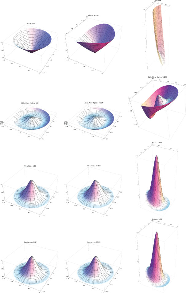
Figure 1: Radial Basis Functions (firts column) and corresponding modified Radial Basis Functions for a material with quadratic variation of k(x) (second column) and exponential variation of k(x) (third column).

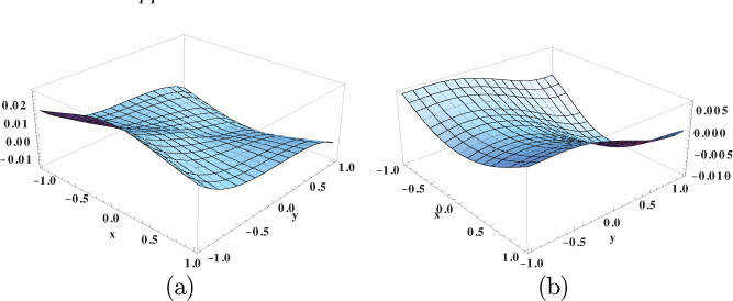
Figure 2: (a) Residual $R$ (x; y) and (b) remainder $U_{R}$ (x; y) approximated by 10 10 Wendland Modified Radial Basis Functions (parameter S $=$ 1.2 for the RBF) for the problem described in [23].

In Figure 2 the residual and the remainder are shown for the collocation point at (0, 0). The residual is computed exactly by the analytical expression in (14) while the remainder $U_{R} (x; y)$ is approximated using a grid of 10 10 Wendland Modified RBFs (parameter S $=$ 1.2 for the RBF). Note that both the residual and the remainder are smooth functions, even around the collocation point (0, 0).

In Figure 3 the Fundamental Solution analytically computed $(U_{e x a c t} (x; y))$ , approximated by the proposed procedure $(U_{a p p r o x} (x; y))$ and their difference $(Δ U = U_{e x a c t} (x; y) - U_{a p p r o x} (x; y))$ are shown for different axes $(x_{1} = c o n s t . a n d x_{2} = c o n s t .) .$ The approximation is carried out using a grid of 10 10 Wendland Modified RBFs. Very similar but slightly different results are obtained using Buhmann Modified RBFs as shown in Figure 4.

It is shown that using both the Wendland RBFs and the Buhmann RBFs, the difference between the exact and approximated FS’s goes to zero as one approaches the collocation point, but it seems that U $_{a p p r o x}$ (x; y) is not a good approximation of $U_{e x a c t}$ (x; y) far from it. However, it can be numerically checked that

\nabla \cdot (k (x) \nabla Δ U (x; y)) = \nabla \cdot (k (x) \nabla [U_{e x a c t} (x; y) - U_{a p p r o x} (x; y)]) \approx 0

(18)

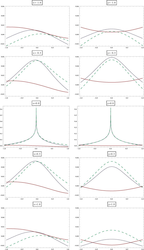
Figure 3: Analytically computed Fundamental Solution (dotted blue line), approximated by the proposed procedure (dashed green line) and their difference (continuos red line) for different axes ( $x_{1}$ $=$ const. and $x_{2}$ $=$ const.). The approximation is carried out using a grid of 10 10 Wendland Modified RBFs.

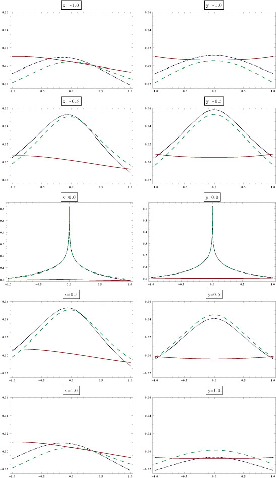
Figure 4: Analytically computed Fundamental Solution (dotted blue line), approximated by the proposed procedure (dashed green line) and their difference (continuos red line) for different axes ( $x_{1} =$ const. and $x_{2} =$ const.). The approximation is carried out using a grid of 10 10 Buhmann Modified RBFs.

This means that $U_{a p p r o x} (x; y)$ is a Fundamental Solution but different from the one provided by $U_{e x a c t} (x; y)$ . Actually, the $U_{a p p r o x} (x; y)$ are different for different RBFs, but in all cases $\nabla \cdot (k (x) \nabla Δ U (x; y)) \approx 0$ .

6 Conclusions

In this paper, a method is proposed and implemented for obtaining Fundamental Solutions in problems with spatially variable material parameters. The method is based in two steps: firstly a Levi Function of the problem is analytically obtained by an iterative procedures, and secondly the remainder of this Levi Function is approximated using particular solutions of the original operator, which are found modifying standard Radial Basis Functions.

The following remarks apply to the present approach:

The technique is easy to implement numerically.
Modified Radial Basis Functions provide very high rates of convergence, but not all standard RBF can be applied, since the ensuing MRBF is not regular for all RBF.
If using a global approximation of the remainder, the kernel matrix M is computed and factorized only once, and therefore the calculation of the Fundamental Solution for any number of collocation points y is not computationally expensive.

The method is validated using the heat transfer problem with variable conductivity. For this problem the Levi Function to the third order is computed and presented in this paper for the first time.

References

[1] Brebbia, C. A. and Domnguez, J. (1989). Boundary elements: An introductory course. McGraw Hill Book Co.

[2] Kausel, E. (2006). Fundamental Solutions in Elastodynamics. A compendium. Cambridge University Press.

[3] Clements, D. L. (1998) Fundamental solutions for second order linear elliptic partial differential equations. Computational Mechanics, 22, 26–31.

[4] Shaw, R. P. (1994). Green’s functions for heterogeneous media potential problems. Engineering Analysis with Boundary Elements, 13, 219–221.

[5] Nardini, D and Brebbia, C. A.(1983). A new approach to free vibration analysis using boundary elements. Applied Mathematical Modelling, 7(3), 157–162.

[6] Gao, X. W. (2002). The radial integration method for evaluation of domain integrals with boundary-only discretization. Engineering Analysis with Boundary Elements, 26 905–916.

[7] Gao, X. W. Zhang, Ch. and Guo, L. (2007). Boundary-only element solutions of 2D and 3D nonlinear and nonhomogeneous elastic problems. Engineering Analysis with Boundary Elements, 31(12), 947–982.

[8] Katsikadelis, J.T. (1994). The Analog Equation Method: A Powerful BEM-based Solution Technique for Solving Linear and Nonlinear Engineering Problems, In: Boundary Element Method XVI, ed. C.A. Brebbia, Computational Mechanics Publications, 167–182.

[9] Riveiro, M.A. and Gallego, R.(2013). Boundary elements and the analog equation method for the solution of elastic problems in 3-D non-homogeneous bodies. Comput. Meth. Appl. Mech. Eng., 263, 12–19.

[10] Levi, E. E. (1909). I problemi dei valori al contorno per le equazioni lineari totalmente ellittiche alle derivate parziali. Memorie della Societa Italiana di Scienze XL, 16, 1–112.

[11] Al-Jawary, M. A. and Wrobel, L. C. (2011). Numerical solution of two-dimensional mixed problems with variable coefficients by the boundary-domain integral and integro-differential equation methods. Engineering Analysis with Boundary Elements, 35, 1279–1287.

[12] Mikhailov, S. E. (2015). Analysis of Segregated Boundary-Domain Integral Equations for Variable-Coefficient Dirichlet and Neumann Problems with General Data. arXiv:1509.03501.

[13] Pomp, A. (1998). The Boundary-Domain Integral Method for Elliptic Systems. Springer-Verlag, Berlin.

[14] Buhmann, M. D. (2003). Radial Basis Functions, Theory and Implementations. Cambridge University Press.

[15] Chen, W. and Tanaka, M. (2002). A meshless, exponential convergence, integration-free, and boundary only RBF technique. Computers and Mathematics with Applications, 43, 379–391.

[16] Golberg, M. A. and Chen, C. S. (1998). The method of fundamental solutions for potential, Helmholtz and diffusion problems. In M. A. Golberg, editor, Boundary Integral Methods: Numerical and Mathematical Aspects, 103–176. WIT Press.

[17] Kansa, E. J. (1990). Multiquadrics – a scattered data approximation scheme with applications to computational fluid dynamics – I. Computers and Mathematics with Application, 19 (8/9), 127–145.

[18] Kansa, E. J. (1990). Multiquadrics – a scattered data approximation scheme with applications to computational fluid dynamics – II. Computers and Mathematics with Application, 19 (8/9), 147–161.

[19] Kupradze, V. D. and Aleksidze, M. A. (1964). The method of functional equations for the approximate solution of certain boundary value problems. U.S.S.R. Computational Mathematics and Mathematical Physics, 4, 82–126.

[20] Gupta, A. and Talha, M. (2015). Recent development in modeling and analysis of functionally graded materials. Progress in Aerospace Sciences, 79, 1–14.

[21] Jha, D. K., Kant, T. and Singn, R. K. (2013). A critical review of recent research on functionally graded plates. Composite Structures, 96, 833–849.

[22] Pomp, A. (1998). Levi Functions for linear elliptic systems with variable coefficients including shell equations. Computational Mechanics, 22, 93–99.

[23] Dumont, N. A. Chaves, R. A. P. and Paulino, G. H. (2002). The hybrid boundary element method applied to functionally graded materials. In C. A. Brebbia, A. Tadeu, V. Popov, editors, Boudary Elements XXIV.

[24] Sutradhar, A. and Paulino, G. H. (1994). A symple boundary element method for problems of non-homogeneous media. International Journal for numerical Methods in Engineering, 60, 2203–2230.

Biographies

Rafael Gallego is full professor at the University of Granada since 1995. He received his Bachelor and Master degrees in Structural and Mechanical Engineering at the University of Sevilla (1987) and got his PhD at the same University in 1990; he was granted a Fulbright postdoctoral scholarship (1990–92) at the Brown University. Among other academic posts, he has been chairman of the Department of Structural and Hydraulic Engineering at the University of Granada since 2000 to 2008 and since 2016 to date. His research work has focused in developing computational models based on Boundary Integral Equations for solid mechanics problem, mainly related to wave propagation in solids, dynamic fracture mechanics and dynamic soil-structure interaction, including resolution of inverse problems to match computational results and experimental ones.

Esther Puertas Garca is permanent lecturer at the University of Granada. She received her Bachelor and Master degrees in Civil Engineering at the University of Granada, and PhD degrees in Civil Engineering from the University of Granada in 2014. She has an extensive teaching, research and professional experience in the Mechanics of Continuous Media and Theory of Structures topics. Her research work concerns the development of computational toolkits for continuum media dynamics. She belongs to the Research Group of Mechanics of Solids and Structures. Her lines of work are based on the study of Integral Equations Methods for advanced applications in Solid Mechanics. She has developed techniques for the analysis of wave propagation problems in two and a half domains.

European Journal of Computational Mechanics, Vol. 28 1&2, 3150.
doi: 10.13052/ejcm1958-5829.28122
© 2019 River Publishers