Analysis of Two- and Three-dimensional Steady-state Thermo-mechanical Problems Including Curved Line/Surface Heat Sources Using the Method of Fundamental Solutions

M. Mohammadi^1,∗, M. R. Hematiyan² and A. Khosravifard²

¹Department of Mechanical Engineering, College of Engineering, Shiraz Branch,
Islamic Azad University, Shiraz, Iran
²Department of Mechanical Engineering, Shiraz University, Shiraz 71936, Iran
E-mail: mehr4457@gmail.com; mohammadi mehrdad@iaushiraz.ac.ir
^*Corresponding Author

Received 05 March 2019; Accepted 28 June 2019;
Publication 05 August 2019

Abstract

In this work, the method of fundamental solutions (MFS) and the method of particular solutions (MPS) are used to solve two and three dimensional steady-state thermoelastic problems involving curved-shape heat sources. The geometrical shape of the heat sources can be very complicated. Each curved heat source is modelled by assembling several simple sources with quadratic shapes. The particular solutions for temperature and stress are presented in simple forms and they are used without considering any internal points or internal cells. Several examples are analysed to demonstrate the efficiency of the presented formulation. Numerical results show that the presented MFS-MPS formulation is very efficient and useful. Unlike the finite element method, only a small number of collocation and source points are sufficient to achieve accurate results in the proposed MFS formulation.

Keywords: Method of fundamental solutions, Curved line heat source, Curved surface heat source, Thermo-mechanical, Meshfree

1 Introduction

In practical thermo-mechanical problems such as infrared heating, electrical heating and laser beam welding, it is necessary to consider concentrated heat sources for accurate modelling of such systems. Only a few analytical solutions are presented yet for these types of problems. For example, [1] presented a general analytical solution for an annular involving a point heat source. [2] presented Green’s functions for some boundary value problems in an infinite plane with a point heat source, and [3] presented Green’s functions for a multi-material domain including a point heat source. Despite these analytical solutions, for complicated practical problems involving concentrated heat sources, numerical methods should be used.

The finite element method (FEM) is a popular numerical method for solving large majority of thermo-mechanical problems. But in the FEM, a concentrated heat source should be modeled as a separated region with a small area. The size of this area affects the accuracy of the analysis and a large number of internal elements and nodes should be used, especially near the heat source region. As a powerful alternative, the boundary element method (BEM) only requires boundary discretization. The BEM, which is based on fundamental solutions, has been used effectively to solve direct and inverse thermo-mechanical problems containing concentrated heat sources. [4] proposed a BEM approach for identification of intensity of point heat sources in time-dependent heat conduction. He tested his proposed method by conducting some 2D experiments [5]. [6] formulated line and distributed heat sources in the BEM analysis of nonlinear heat conduction problems in two and three dimensions. They also used the proposed method for inverse non-linear heat conduction analysis [7]. There is no need for domain discretization in their proposed method. [8] used the BEM for thermoelastic analysis of two-dimensional anisotropic media involving concentrated heat sources. They converted domain integrals to boundary integrals in their formulation. In another work, [9] presented a BEM approach for heat conduction in anisotropic non-homogeneous media involving internal point heat sources. They used the direct domain mapping (DDM) technique to enable the exact volume integral transformation. [10] presented a BEM formulation with no need to any internal points or cells for 2D and 3D thermo-elastic problems including point, straight line and flat surface heat sources. They considered a linear variation for the strength of heat sources in their formulation. [11] implemented curved line heat sources with arbitrary variations in 2D and 3D isotropic domains by considering several quadratic heat sources.

Another efficient numerical method is the method of fundamental solutions (MFS), which is used in the present work. Similar to the BEM, the MFS is a boundary-type technique and it is applicable when a fundamental solution of the problem is known. However, the MFS does not require any mesh and it is an integration-free method. Therefore, developing computer codes for the MFS is much simpler than the BEM and it provides very good results with low computational cost [12, 13]. The MFS is a simple method in which the solution of the problem is expressed in terms of fundamental solutions with some unknown coefficients. The singular points of the fundamental solutions are positioned on a boundary outside the body. The intensities of the MFS sources are unknown and are determined by satisfying boundary conditions on some collocation points on the boundary of the body. After the first numerical implementation of the MFS by [14], various applications of this method have been presented in the literature. An overview can be found in the works of [15–18].

The governing equations of the steady-state thermo-elasticity involving heat sources are the heat conduction equation including the heat source term (a standard Poisson equation) and the Navier equations with thermal effects. To solve these equations using the MFS, particular solutions corresponding to heat source terms in addition to homogeneous solutions of the equations should be found. The MFS in conjunction with the dual reciprocity method (DRM) [19] was used by [20] for solving Poisson’s equation, by [21] to solve two-dimensional thermo-elasticity with general body forces, by [22] for thermo-mechanical analysis of functionally graded materials and by [23] to solve three-dimensional thermo-elasticity with arbitrary body forces. Another similar approach is the MFS in combination with the so called method of particular solutions (MPS). The MFS-MPS was used by [24] to solve Poisson’s equation, by [25] for thermo-elastic problems in axisymmetric domains, by [26] to solve two-dimensional thermoelasticity, by [27] for three-dimensional inverse thermoelasticity, by [28] to solve two-dimensional thermoelasticity with the non-singular MFS (NMFS), and by [13] for steady state heat conduction in 2D and 3D isotropic domains involving curved heat sources.

To the authors’ best knowledge, the MFS formulation for thermo-elastic problems involving internal curved heat sources has not been presented yet. The method proposed by [13] for heat conduction analysis is developed here for thermo-mechanical problems. In the present work, the MFS-MPS is used for 2D and 3D analysis of steady-state thermo-mechanical problems involving curved line/surface heat sources.The particular solutions associated with the heat source effect are presented in simple forms. They are calculated without considering any internal points or internal cells and therefore the attractiveness of the MFS as a boundary-type mesh-free method is preserved. Several numerical example problems are presented to demonstrate the advantages of the proposed MFS in comparison with the BEM and the finite element method (FEM).

2 Basic Equations and Formulation

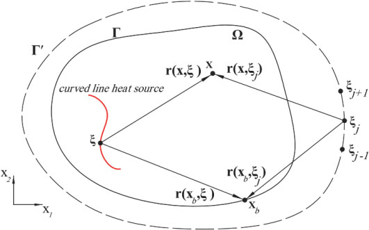
Figure 1: Domain, main boundary, pseudo boundary, and a curved line heat source.

Consider a medium $\Omega$ with its boundary $\Gamma$ (Figure 1). In the presence of heat sources, the governing equation of steady-state heat conduction can be expressed as

$${\nabla }^2\tau \left(\mathbf{\text{x}}\right)=-\frac{s\left(\mathbf{\text{x}}\right)}{k}in\Omega$$

(1)

The boundary conditions can be written as

$$f_1\left({\mathbf{\text{x}}}_b\right)\tau \left({\mathbf{\text{x}}}_b\right)+f_2\left({\mathbf{\text{x}}}_b\right)\frac{\partial \tau \left({\mathbf{\text{x}}}_b\right)}{\partial n}=f_3\left({\mathbf{\text{x}}}_b\right)on\Gamma$$

(2)

where $f_1$, $f_2$ and $f_3$ are given functions on the boundary, ${\nabla }^2$ is the Laplace operator, n is the direction normal to the boundary, x is a point in the domain, ${\mathbf{\text{x}}}_b$ is a point on the boundary, $\tau$ is the temperature, $s\left(\mathbf{\text{x}}\right)$ is a known function describing the heat source distribution in the domain and $k$ is the thermal conductivity.

Navier equations for two and three dimensional problems with consideration of the thermal effects are given as:

$$G{\nabla }^2{u}_i\left(\mathbf{\text{x}}\right)+G1-2\bar{\nu }\sum \underset{}{\overset{}{}}j=1d\left({\partial }^2{u}_j\left(\mathbf{\text{x}}\right)\partial x_i\partial x_j\right)-\bar{\gamma }\partial \tau \left(\mathbf{\text{x}}\right)\partial x_i=0$$

(3)

where d is the dimension of the problem, i.e. d $=$ 2 for a 2D problem and d $=$ 3 for a 3D problem, and i $=$ 1, 2 for 2D problems and i $=$ 1, 2, 3 for 3D problems.

Mechanical boundary conditions can be expressed as follows:

$$\begin{array}{r}\begin{array}{rl}{u}_i({\mathbf{\text{x}}}_b)& =g_i({\mathbf{\text{x}}}_b)\mathrm{o}\mathrm{n}{\mathrm{\Gamma <!--\; \Gamma \; -->}}_1(4)\\ t_i({\mathbf{\text{x}}}_b)& =h_i({\mathbf{\text{x}}}_b)\mathrm{o}\mathrm{n}{\mathrm{\Gamma <!--\; \Gamma \; -->}}_2\end{array}\end{array}$$

where ${\mathrm{\Gamma <!--\; \Gamma \; -->}}_1\cup <!--\; \cup \; -->{\mathrm{\Gamma <!--\; \Gamma \; -->}}_2=\mathrm{\Gamma <!--\; \Gamma \; -->}.u_{i}and{t}_i$ are the components of displacement vector and traction vector, respectively, G is the modulus of rigidity and $g_i$ and h_i are prescribed functions on the boundary. In Equation (3) $\stackrel{¯<!--\; ¯\; -->}{\mathrm{\gamma <!--\; \gamma \; -->}}=2G\stackrel{¯<!--\; ¯\; -->}{\mathrm{\alpha <!--\; \alpha \; -->}}(1+\stackrel{¯<!--\; ¯\; -->}{\mathrm{\nu <!--\; \nu \; -->}})/\phantom{2G\stackrel{¯<!--\; ¯\; -->}{\mathrm{\alpha <!--\; \alpha \; -->}}(1+\stackrel{¯<!--\; ¯\; -->}{\mathrm{\nu <!--\; \nu \; -->}})(1-<!--\; -\; -->2\stackrel{¯<!--\; ¯\; -->}{\mathrm{\nu <!--\; \nu \; -->}})}(1-<!--\; -\; -->2\stackrel{¯<!--\; ¯\; -->}{\mathrm{\nu <!--\; \nu \; -->}})$, where

$$\begin{array}{rcl}\stackrel{¯<!--\; ¯\; -->}{\mathrm{\nu <!--\; \nu \; -->}}& =& \{\begin{array}{ll}\mathrm{\nu <!--\; \nu \; -->}& \mathrm{p}\mathrm{l}\mathrm{a}\mathrm{n}\mathrm{e}\mathrm{s}\mathrm{t}\mathrm{r}\mathrm{a}\mathrm{i}\mathrm{n}\mathrm{a}\mathrm{n}\mathrm{d}3\mathrm{D}\\ \mathrm{\nu <!--\; \nu \; -->}/(1+\mathrm{\nu <!--\; \nu \; -->})& \mathrm{p}\mathrm{l}\mathrm{a}\mathrm{n}\mathrm{e}\mathrm{s}\mathrm{t}\mathrm{r}\mathrm{e}\mathrm{s}\mathrm{s}\end{array}\\ \\ \stackrel{¯<!--\; ¯\; -->}{\mathrm{\alpha <!--\; \alpha \; -->}}& =& \{\begin{array}{ll}\mathrm{\alpha <!--\; \alpha \; -->}& \mathrm{p}\mathrm{l}\mathrm{a}\mathrm{n}\mathrm{e}\mathrm{s}\mathrm{t}\mathrm{r}\mathrm{a}\mathrm{i}\mathrm{n}\mathrm{a}\mathrm{n}\mathrm{d}3\mathrm{D}\\ \mathrm{\alpha <!--\; \alpha \; -->}(1+\mathrm{\nu <!--\; \nu \; -->})/(1+2\mathrm{\nu <!--\; \nu \; -->})& \mathrm{p}\mathrm{l}\mathrm{a}\mathrm{n}\mathrm{e}\mathrm{s}\mathrm{t}\mathrm{r}\mathrm{e}\mathrm{s}\mathrm{s}\end{array}\end{array}$$

(5)

where $\alpha$ represents the coefficient of linear thermal expansion and $\nu$ is the Poisson’s ratio.

The solution of Equation (1) in the MFS is represented as follows:

$$\tau \left(\mathbf{\text{x}}\right)=\sum _{l=1}^N{a}_l{\tau }^{*}\left(\mathbf{\text{x}},{\xi }_l\right))+{\tau }^p\left(\mathbf{\text{x}}\right)$$

(6)

where $\xi {}_{}l$ and $a_l$ are the location and intensity of the lth source point on the pseudo boundary ${\Gamma }^{\prime }$, respectively, and N is the number of source points. The fundamental solution of the Laplace equation is denoted by ${\tau }^{*}$ and is expressed as

$$\begin{array}{rcll}{\tau }^{*}\left(\mathbf{\text{x}},{\xi }_l\right)& =\frac{-1}{2\pi }ln\left(r\left(\mathbf{\text{x}},{\xi }_l\right)\right)for2D& & \text{(7)}\\ {\tau }^{*}\left(\mathbf{\text{x}},{\xi }_l\right)& =\frac{1}{4\pi r\left(\mathbf{\text{x}},{\xi }_l\right)}for3D\end{array}$$

where r is the magnitude of the vector $\mathbf{\text{r}}$, which represents the distance between the source point ${\xi }_l$ to the point x.

${\tau }^p\left(\mathbf{\text{x}}\right)$ in Equation (6) is the particular solution and it can be obtained by constructing the associated Newton potential in the following domain integral form [15]:

$${\tau }^p\left(\mathbf{\text{x}}\right)=\frac{1}{k}\underset{\Omega }{\int }s\left(\xi \right){\tau }^{*}\left(\mathbf{\text{x}},\xi \right)dV\left(\xi \right)$$

(8)

Considering $N$ collocation points on the main boundary and satisfying the thermal boundary conditions at these points, the coefficients $a_l$ can be determined.

Considering thermal effects in the Navier equation, the solution of this equation can be represented as follows:

$$u_i\left(\mathbf{\text{x}}\right)=u_i^h\left(\mathbf{\text{x}}\right)+u_i^p\left(\mathbf{\text{x}}\right)$$

(9)

The components of the homogeneous displacement vector (solution of the Navier equation without thermal terms) are expressed as follows [21]:

$$\begin{array}{r}{u}_i^h\left(\mathbf{\text{x}}\right)=\sum _{l=1}^N\left[c_l{U}_{1i}^{*}\left(\mathbf{\text{x}},{\xi }_l\right)+c_{l+N}{U}_{2i}^{*}\left(\mathbf{\text{x}},{\xi }_l\right)\right]\left(for2D\right)\left(6\right)\\ u_i^h\left(\mathbf{\text{x}}\right)=\sum _{l=1}^N\left[c_l{U}_{1i}^{*}\left(\mathbf{\text{x}},{\xi }_l\right)+c_{l+N}{U}_{2i}^{*}\left(\mathbf{\text{x}},{\xi }_l\right)+c_{l+2N}{U}_{3i}^{*}\left(\mathbf{\text{x}},{\xi }_l\right)\right]\left(for3D\right)\end{array}$$

(10)

$$$$

where:

$$\begin{array}{r}{U}_{ij}^{*}=\frac{1}{8\pi \left(1-\bar{\nu }\right)G}\left[\left(3-4\bar{\nu }\right)ln\left(\frac{1}{r}\right){\delta }_{ij}+r_{,i}{r}_{,j}\right]\left(for2D\right)\left(8\right)U\dot{}ijˆ*\\ =\frac{1}{16\pi \left(1-\bar{\nu }\right)Gr}\left[\left(3-4\bar{\nu }\right){\delta }_{ij}+r_{,i}{r}_{,j}\right]\left(for3D\right)\end{array}$$

(11)

$$$$

in which

$$r_{,i}=\frac{r_i}{r}$$

(12)

where $r_i$ are the elements of the vector $\mathbf{\text{r}}$.

The coefficients $c_l$ in Equation (10) are unknowns, which can be found by applying boundary conditions. The components of the particular displacement vector (solution of the Navier equations with thermal terms) can be represented by the following equation:

$$u_i^p\left(\mathbf{\text{x}}\right)=\frac{1}{Ā}\sum _{l=1}^N\left[a_l{r}_i\left(\mathbf{\text{x}},{\xi }_l\right){\tau }^{*}\left(\mathbf{\text{x}},{\xi }_l\right)\right]+\frac{1}{kĀ}\underset{\Omega }{\int }s\left(\xi \right)r_i\left(\mathbf{\text{x}},\xi \right){\tau }^{*}\left(\mathbf{\text{x}},\xi \right)dV\left(\xi \right)$$

(13)

where:

$$Ā=\frac{4G\left(1-\bar{\nu }\right)}{\bar{\gamma }\left(1-2\bar{\nu }\right)}$$

(14)

The components of the traction vector at boundary points can be calculated as follows:

$$t_i\left({\mathbf{\text{x}}}_b\right)=t_i^h\left({\mathbf{\text{x}}}_b\right)+t_i^p\left({\mathbf{\text{x}}}_b\right)$$

(15)

where $t_i^h$ and $t_i^p$ are components of the homogeneous traction vector and the particular traction vector, respectively. The components of homogeneous traction vector can be derived from the following equations [21]:

$$\begin{array}{r}{t}_i^h\left({\mathbf{\text{x}}}_b\right)=\sum _{l=1}^N\left[c_l{P}_{1i}^{*}\left({\mathbf{\text{x}}}_b,{\xi }_l\right)+c_{l+N}{P}_{2i}^{*}\left({\mathbf{\text{x}}}_b,{\xi }_l\right)\right]\left(for2D\right)\left(14\right)t\dot{}iˆh\left(x\dot{}b\right)\\ =\sum _{l=1}^N\left[c_l{P}_{1i}^{*}\left({\mathbf{\text{x}}}_b,{\xi }_l\right)+c_{l+N}{P}_{2i}^{*}\left({\mathbf{\text{x}}}_b,{\xi }_l\right)+c_{l+2N}{P}_{3i}^{*}\left({\mathbf{\text{x}}}_b,{\xi }_l\right)\right]\left(15\right)\\ \left(for3D\right)\end{array}$$

(16)

where: P˙ijˆ*=-1 $2^d\pi \left(1-\bar{\nu }\right)r^{\left(d-1\right)}$ ((1-2ν̄)δij+dr,jr,i) ∂r ∂n-(1-2ν̄) (r,inj-r,jni)

$$$$

(17)

in which, $n_i$ are the elements of the unit vector $n$, normal to the boundary.

The components of the particular traction vector can be calculated as follows:

$$t_i^p\left({\mathbf{\text{x}}}_b\right)={\sigma }_{ij}^p\left({\mathbf{\text{x}}}_b\right)n_j\left({\mathbf{\text{x}}}_b\right)$$

(18)

In order to calculate the components of the particular stress tensor ${\sigma }_{ij}^p$ at a point, the following stress-strain relation can be used:

$${\sigma }_{ij}^p\left(\mathbf{\text{x}}\right)=2G\left[{\epsilon }_{ij}^p\left(\mathbf{\text{x}}\right)+\frac{\bar{\nu }}{1-2\bar{\nu }}{\epsilon }_{kk}^p\left(\mathbf{\text{x}}\right){\delta }_{ij}\right]-\bar{\gamma }\tau \left(\mathbf{\text{x}}\right){\delta }_{ij}$$

(19)

The components of the particular strain tensor ${\epsilon }_{ij}^p$ at a point can be determined using the strain-displacement relation as

$$\begin{array}{r}{\epsilon }_{ij}^p\left(\mathbf{\text{x}}\right)=\frac{1}{2}\left(u_{i,j}^p\left(\mathbf{\text{x}}\right)+u_{j,i}^p\left(\mathbf{\text{x}}\right)\right)\left(20\right)=\\ \frac{1}{Ā}\sum _{l=1}^N\left[a_l\left({\tau }^{*}\left(\mathbf{\text{x}},{\xi }_l\right){\delta }_{ij}-\frac{r_i\left(\mathbf{\text{x}},{\xi }_l\right)r_j\left(\mathbf{\text{x}},{\xi }_l\right)}{2^{\left(d-1\right)}\pi r^d\left(\mathbf{\text{x}},{\xi }_l\right)}\right)\right]\left(21\right)\\ +\frac{1}{kĀ}\underset{\Omega }{\int }s\left(\xi \right)\left({\tau }^{*}\left(\mathbf{\text{x}},\xi \right){\delta }_{ij}-\frac{r_i\left(\mathbf{\text{x}},\xi \right)r_j\left(\mathbf{\text{x}},\xi \right)}{2^{\left(d-1\right)}\pi r^d\left(\mathbf{\text{x}},\xi \right)}\right)dV\left(\xi \right)\end{array}$$

(20)

For calculation of stress tensor components at a point of the domain, the following equation can be used:

$${\sigma }_{ij}^{}\left(\mathbf{\text{x}}\right)={\sigma }_{ij}^h\left(\mathbf{\text{x}}\right)+{\sigma }_{ij}^p\left(\mathbf{\text{x}}\right)$$

(21)

In which, the components of the homogeneous stress tensor ${\sigma }_{ij}^h$ can be calculated as follows [21]:

$$\begin{array}{r}{\sigma }_{ij}^h\left(\mathbf{\text{x}}\right)=\sum _{l=1}^N\left[c_l{\Psi }_{1ij}^{*}\left(\mathbf{\text{x}},{\xi }_l\right)+c_{l+N}{\Psi }_{2ij}^{*}\left(\mathbf{\text{x}},{\xi }_l\right)\right]\left(for2D\right)\left(24\right){\sigma }_{ij}^h\left(\mathbf{\text{x}}\right)\\ =\sum _{l=1}^N\left[c_l{\Psi }_{1ij}^{*}\left(\mathbf{\text{x}},{\xi }_l\right)+c_{l+N}{\Psi }_{2ij}^{*}\left(\mathbf{\text{x}},{\xi }_l\right)+c_{l+2N}{\Psi }_{3ij}^{*}\left(\mathbf{\text{x}},{\xi }_l\right)\right]\left(25\right)\\ \left(for3D\right)\end{array}$$

(22)

where: ${\Psi }_{ijk}^{*}=\frac{-1}{2^d\pi \left(1-\bar{\nu }\right)r^{\left(d-1\right)}}\left[\left(1-2\bar{\nu }\right)\left(r_{,j}{\delta }_{ik}+r_{,k}{\delta }_{ij}-r_{,i}{\delta }_{jk}\right)+\right.\left.d{r}_{,i}{r}_{,j}{r}_{,k}\right]$

(23)

As it can be seen in Equations (8), (13) and (20), the particular solutions associated with the heat source effect are represented by domain integrals. In the next section, these integrals are calculated for curved line/surface heat sources without any need for internal cells or internal points.

3 Formulations for Heat Sources Concentrated on a Curved Line/Surface

In this section, the particular solutions associated with curved line/surface heat sources in the MFS are presented. For the 2D case, curved line sources and for the 3D case, both curved line and curved surface sources are considered.

3.1 Curved Line Heat Source in Two-dimensional Problems

Any curved line heat source can be discretized by several quadratic segments. As shown in Figure 2, each segment has a quadratic shape and is represented by three points. The domain integrals in Equations (8), (13) and (20) for the 2D case, are converted to integrals over the quadratic segment as follows:

$$\begin{array}{rcll}{I}_T\left(\mathbf{\text{x}}\right)& =\frac{-1}{2\pi k}\underset{l_{source}}{\int }s\left(\xi \right)ln\left[r\left(\mathbf{\text{x}},\xi \right)\right]dl& & \\ I_u\left(\mathbf{\text{x}}\right)& =\frac{-1}{2\pi kĀ}\underset{l_{source}}{\int }s\left(\xi \right)r_i\left(\mathbf{\text{x}},\xi \right)ln\left[r\left(\mathbf{\text{x}},\xi \right)\right]dl& & \\ I_{\epsilon }\left(\mathbf{\text{x}}\right)& =\frac{-1}{2\pi kĀ}\underset{l_{source}}{\int }s\left(\xi \right)\left(ln\left[r\left(\mathbf{\text{x}},\xi \right)\right]{\delta }_{ij}+\frac{r_i\left(\mathbf{\text{x}},\xi \right)r_j\left(\mathbf{\text{x}},\xi \right)}{r^2\left(\mathbf{\text{x}},\xi \right)}\right)dl\end{array}$$

(24)

where $dl$ is an infinitesimal element on the quadratic segment, $r\left(\mathbf{\text{x}},\xi \right)=\sqrt{{\left(x-x_s\right)}^2+{\left(y-y_s\right)}^2}$ is the distance between the field point $\mathbf{\text{x}}=\left(x,y\right)$ and the source points $\xi =\left(x_s,y_s\right)$ on the quadratic line heat source, $r_1\left(\mathbf{\text{x}},\xi \right)=\left(x-x_s\right)$, and $r_2\left(\mathbf{\text{x}},\xi \right)=\left(y-y_s\right)$.

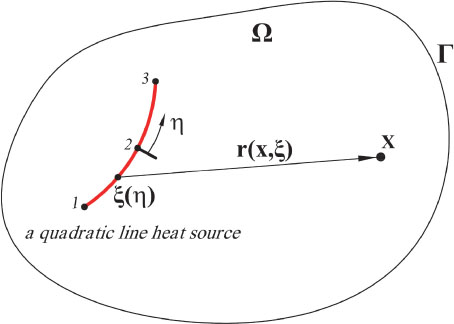
Figure 2: A curved line heat source with quadratic shape and its dimensionless local coordinate.

The coordinates of the point $\xi =\left(x_s,y_s\right)$ on the quadratic segment can be expressed as

$$x_s=\left(N_1{x}_1+N_2{x}_2+N_3{x}_3\right)y_s=\left(N_1{y}_1+N_2{y}_2+N_3{y}_3\right)$$

(25)

where $\left(x_1,y_1\right)$, $\left(x_2,y_2\right)$ and $\left(x_3,y_3\right)$ are respectively, the coordinates of the starting point, the middle point and the end point of the quadratic segment and $N_1$, $N_2$ and $N_3$ are the quadratic Lagrangian shape functions. These shape functions can be expressed as follows [29]:

$$N_1=\frac{1}{2}\eta \left(\eta -1\right)N_2=-\left(\eta +1\right)\left(\eta -1\right)N_3=\frac{1}{2}\eta \left(\eta +1\right)$$

(26)

where $-1\le \eta \le +1$ is a dimensionless local coordinate shown in Figure 2. Using Equation (25), the integrals in Equation (24) are converted to the following integrals:

$$\begin{array}{r}{I}_T\left(\mathbf{\text{x}}\right)=\frac{-1}{2\pi k}\underset{-1}{\overset{1}{\int }}s\left(\eta \right)ln\left[r\left(\eta \right)\right]Jd\eta \\ I_u\left(\mathbf{\text{x}}\right)=\frac{-1}{2\pi kĀ}\underset{-1}{\overset{1}{\int }}s\left(\eta \right)r_i\left(\eta \right)ln\left[r\left(\eta \right)\right]Jd\eta \\ I_{\epsilon }\left(\mathbf{\text{x}}\right)=\frac{-1}{2\pi kĀ}\underset{-1}{\overset{1}{\int }}s\left(\eta \right)\left(ln\left[r\left(\eta \right)\right]{\delta }_{ij}+\frac{r_i\left(\eta \right)r_j}{r^2\left(\eta \right)}\right)Jd\eta \end{array}$$

(27)

where J is the Jacobian of transformation.

The integrals in Equation (27) can be calculated using conventional numerical integration methods such as the Gaussian quadrature method (GQM). It should be noted that if the field point $\mathbf{\text{x}}=\left(x,y\right)$ is exactly on the line source, the integrals in Equation (27) will be weakly singular with a finite value. In other words, in the two-dimensional case, stress, displacement and temperature have finite values at points exactly on the curved line heat source. In this case, the integral in Equation (27) can be calculated by various methods such as the weighted Gaussian integration [30], transformation of variable [31] and subtraction of singularity [32] methods. In this research, weighted Gaussian integration method has been used.

3.2 Curved Line Heat Source in 3D Problems

Similar to the 2D case, any curved line heat source in 3D is discretized by some heat sources with quadratic shapes. The domain integrals in Equations (8), (13) and (20) for the 3D case, are converted to integrals on the quadratic segment as follows:

$$\begin{array}{rcll}{I}_T\left(\mathbf{\text{x}}\right)& =\frac{1}{4\pi k}\underset{l_{source}}{\int }\frac{s\left(\xi \right)}{r\left(\mathbf{\text{x}},\xi \right)}dl& & \\ I_u\left(\mathbf{\text{x}}\right)& =\frac{1}{4\pi kĀ}\underset{l_{source}}{\int }s\left(\xi \right)\frac{r_i\left(\mathbf{\text{x}},\xi \right)}{r\left(\mathbf{\text{x}},\xi \right)}dl& & \\ I_{\epsilon }\left(\mathbf{\text{x}}\right)& =\frac{1}{4\pi kĀ}\underset{l_{source}}{\int }s\left(\xi \right)\left(\frac{{\delta }_{ij}}{r\left(\mathbf{\text{x}},\xi \right)}-\frac{r_i\left(\mathbf{\text{x}},\xi \right)r_j\left(\mathbf{\text{x}},\xi \right)}{r^3\left(\mathbf{\text{x}},\xi \right)}\right)dl\end{array}$$

(28)

where $r\left(\mathbf{\text{x}},\xi \right)=\sqrt{{\left(x-x_s\right)}^2+{\left(y-y_s\right)}^2+{\left(z-z_s\right)}^2}$ is the distance between the field point $\mathbf{\text{x}}=\left(x,y,z\right)$ and the source points $\xi =\left(x_s,y_s,z_s\right)$ on the quadratic line heat source, $r_1\left(\mathbf{\text{x}},\xi \right)=\left(x-x_s\right)$, $r_2\left(\mathbf{\text{x}},\xi \right)=\left(y-y_s\right)$, and $r_3\left(\mathbf{\text{x}},\xi \right)=\left(z-z_s\right)$.

Each quadratic segment is discretized by three points, i.e. $\left(x_1,y_1,z_1\right)$ at the starting point, $\left(x_2,y_2,z_2\right)$ at the middle point, and $\left(x_3,y_3,z_3\right)$ at the end point. The coordinates of the points $\xi =\left(x_s,y_s,z_s\right)$ on the quadratic segment can be expressed as follows:

$$\begin{array}{r}{x}_s=\left(N_1{x}_1+N_2{x}_2+N_3{x}_3\right),y_s=\left(N_1{y}_1+N_2{y}_2+N_3{y}_3\right),\\ z_s=\left(N_1{z}_1+N_2{z}_2+N_3{z}_3\right)\left(29\right)\end{array}$$

where $N_1$, $N_2$ and $N_3$ are the quadratic Lagrangian shape functions as given in Equation (26).

Using Equation (29), the integrals in Equation (28) are converted to the following integrals:

$$\begin{array}{r}{I}_T\left(\mathbf{\text{x}}\right)=\frac{1}{4\pi k}\underset{-1}{\overset{1}{\int }}\frac{s\left(\eta \right)}{r\left(\eta \right)}\\ Jd\eta I_u\left(\mathbf{\text{x}}\right)=\frac{1}{4\pi kĀ}\underset{-1}{\overset{1}{\int }}s\left(\eta \right)\frac{r_i\left(\eta \right)}{r\left(\eta \right)}Jd\eta \\ I_{\epsilon }\left(\mathbf{\text{x}}\right)=\frac{1}{4\pi kĀ}\underset{-1}{\overset{1}{\int }}s\left(\eta \right)\left(\frac{{\delta }_{ij}}{r\left(\eta \right)}-\frac{r_i\left(\eta \right)r_j\left(\eta \right)}{r^3\left(\eta \right)}\right)Jd\eta \end{array}$$

(30)

The integrals in Equation (30) can be calculated using conventional numerical integration methods such as the Gaussian quadrature method (GQM). It should be noted that if the field point $\mathbf{\text{x}}=\left(x,y,z\right)$ is exactly on the curved line heat source, the first and the third integrals in Equation (30) will be strongly singular without any finite values, but the second integral in Equation (30) will be weakly singular with a finite value. In other words, in the three-dimensional case, at a point on a curved line heat source, the displacement has a finite value but the temperature and the stress go to infinity.

3.3 Curved Surface Heat Source in 3D Problems

We consider an arbitrary heat source distributed over a curved surface in a 3D domain. Each surface heat source can be divided into several quadrilateral surface heat sources. Each quadrilateral surface heat source has a quadratic shape. A curved surface heat source and one of its quadratic segments are shown in Figure 3.

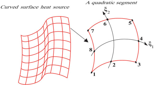
Figure 3: An arbitrary curved surface heat source and a quadratic segment with its local coordinates.

The domain integrals in Equations (8), (13) and (20) for the 3D case, are converted to integrals on the surface of the quadratic segment as follows:

$$\begin{array}{rcll}{I}_T\left(\mathbf{\text{x}}\right)& =\frac{1}{4\pi k}\underset{A_{source}}{\int }\frac{s\left(\xi \right)}{r\left(\mathbf{\text{x}},\xi \right)}dA& & \\ I_u\left(\mathbf{\text{x}}\right)& =\frac{1}{4\pi kĀ}\underset{A_{source}}{\int }s\left(\xi \right)\frac{r_i\left(\mathbf{\text{x}},\xi \right)}{r\left(\mathbf{\text{x}},\xi \right)}dA& & \\ I_{\epsilon }\left(\mathbf{\text{x}}\right)& =\frac{1}{4\pi kĀ}\underset{A_{source}}{\int }s\left(\xi \right)\left(\frac{{\delta }_{ij}}{r\left(\mathbf{\text{x}},\xi \right)}-\frac{r_i\left(\mathbf{\text{x}},\xi \right)r_j\left(\mathbf{\text{x}},\xi \right)}{r^3\left(\mathbf{\text{x}},\xi \right)}\right)dA\end{array}$$

(31)

where $dA$ is an infinitesimal area element on the quadratic surface heat source and $r\left(\mathbf{\text{x}},\xi \right)$ is the distance between the field point $\mathbf{\text{x}}=\left(x,y,z\right)$ and the source points $\xi =\left(x_s,y_s,z_s\right)$ on the quadratic surface heat source. As shown in Figure 3, each quadratic surface heat source is represented by 8 points and a set of local coordinates $\left({\xi }_1,{\xi }_2\right)$, which vary between $-$1 and 1. $x_s$, $y_s$, and $z_s$ can be expressed in terms of the 8 Lagrangian shape functions as follows:

$$\begin{array}{r}{x}_s\left({\xi }_1,{\xi }_2\right)=\sum _{i=1}^8{N}_i\left({\xi }_1,{\xi }_2\right)x_i,y_s\left({\xi }_1,{\xi }_2\right)=\sum _{i=1}^8{N}_i\left({\xi }_1,{\xi }_2\right)y_i,\\ z_s\left({\xi }_1,{\xi }_2\right)=\sum _{i=1}^8{N}_i\left({\xi }_1,{\xi }_2\right)z_i\end{array}$$

(32)

$$$$

where $\left(x_i,y_i,z_i\right)$ are the coordinates of the 8 points on the heat source. The shape functions N ${}_i$ in terms of ${\xi }_1$ and ${\xi }_2$ are expressed as follows [29]:

$$\begin{array}{r}{N}_1=\frac{-1}{4}\left(1-{\xi }_1\right)\left(1-{\xi }_2\right)\left(1+{\xi }_1+{\xi }_2\right),N_2=\frac{1}{2}\left(1-{\xi }_1^2\right)\left(1-{\xi }_2\right),\left(6\right)N\dot{}3\\ =\frac{-1}{4}\left(1+{\xi }_1\right)\left(1-{\xi }_2\right)\left(1-{\xi }_1+{\xi }_2\right),N_4=\frac{1}{2}\left(1+{\xi }_1\right)\left(1-{\xi }_2^2\right),\left(7\right)N\dot{}5\\ =\frac{-1}{4}\left(1+{\xi }_1\right)\left(1+{\xi }_2\right)\left(1-{\xi }_1-{\xi }_2\right),N_6=\frac{1}{2}\left(1-{\xi }_1^2\right)\left(1+{\xi }_2\right),\left(8\right)N\dot{}7\\ =\frac{-1}{4}\left(1-{\xi }_1\right)\left(1+{\xi }_2\right)\left(1+{\xi }_1-{\xi }_2\right),N_8=\frac{1}{2}\left(1-{\xi }_1\right)\left(1-{\xi }_2^2\right).\end{array}$$

(33)

Using Equation (32), the integrals in Equation (31) are converted to the following integrals:

$$\begin{array}{rcll}{I}_T\left(\mathbf{\text{x}}\right)& =\frac{1}{4\pi k}\underset{-1}{\overset{1}{\int }}\underset{-1}{\overset{1}{\int }}\frac{s\left({\xi }_1,{\xi }_2\right)}{r\left({\xi }_1,{\xi }_2\right)}Jd{\xi }_{1}d{\xi }_2& & \\ I_u\left(\mathbf{\text{x}}\right)& =\frac{1}{4\pi kĀ}\underset{-1}{\overset{1}{\int }}\underset{-1}{\overset{1}{\int }}s\left({\xi }_1,{\xi }_2\right)\frac{r_i\left({\xi }_1,{\xi }_2\right)}{r\left({\xi }_1,{\xi }_2\right)}Jd{\xi }_{1}d{\xi }_2& & \\ I_{\epsilon }\left(\mathbf{\text{x}}\right)& =\frac{1}{4\pi kĀ}\underset{-1}{\overset{1}{\int }}\underset{-1}{\overset{1}{\int }}s\left({\xi }_1,{\xi }_2\right)& & \\ & \left(\frac{{\delta }_{ij}}{r\left({\xi }_1,{\xi }_2\right)}-\frac{r_i\left({\xi }_1,{\xi }_2\right)r_j\left({\xi }_1,{\xi }_2\right)}{r^3\left({\xi }_1,{\xi }_2\right)}\right)Jd{\xi }_{1}d{\xi }_2\end{array}$$

(34)

The integrals in Equation (34) can be calculated using standard 2D numerical integration methods such as the GQM. In the cases that the field point $\mathbf{\text{X}}$ is exactly on the surface of the heat source, the integrals in Equation (34) will be weakly singular with a finite value. In other words, in the three-dimensional case, the temperatures, displacements and stresses at points on a surface heat source have finite values. In this case, the integrals in Equation (34), which is weakly singular, can be calculated by various methods such as the transformation of variable and subtraction of singularity methods [32]. In this research, the method of transformation of variable has been used for such cases.

4 Numerical Examples

To verify the proposed MFS formulation, four thermo-mechanical examples are presented. In two-dimensional examples, curved line heat sources and in three-dimensional examples curved line and curved surface heat sources are considered. In the MFS modelling of all examples, the location of source points and collocation points are determined according to the procedure proposed by [33]. In this procedure, a “location parameter” for a source point is defined as the ratio of the distance from the source point to its corresponding collocation point to the distance from the same source point to the neighbouring collocation point [33]. It is recommended that the value of the location parameter be greater than a lower bound to obtain solutions without undesired oscillations. In this work, the locations of source points are determined in a way that the value of the location parameter of source points would be greater than 0.85.

In all examples, the results computed by the present MFS are compared with those of the FEM with a fine mesh as a reference solution. Also in the first example, the BEM results are included. The software package MATLAB is used for writing MFS and BEM source codes and ANSYS package is used for the FE analyses. In all examples, it is assumed that $k=60W∕m{}^{\circ }C$, $\alpha =11.7\times 10^{-6}1{∕}^{\circ }C$, $E=200GPa$ and $\nu =0.3$.

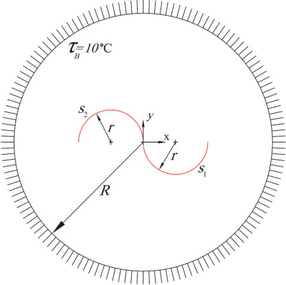
Figure 4: The boundary conditions and the curved line heat sources in a circular domain.

4.1 Two-dimensional Examples

In the two-dimensional examples the state of plane strain is considered. The first 2D example deals with a circular domain with radius $R=0.5m$, which is centred at $\left(0,0\right)$. According to Figure 4, boundary conditions are ${\tau }_B=10{}^{\circ }C$ and $u_x=u_y=0$. The domain involves two semi-circular heat sources with radius of $r=0.125m$ and centres at $\left(0.125,0\right)$ and $\left(-0.125,0\right)$. Their intensity functions are as follows:

$$s_1=16000x+4000W∕m,s_2=-16000x+4000W∕m$$

(35)

In the MFS modelling of the problem, only 8 boundary points and 8 source points are used. The pseudo boundary is considered as a circle with radius of $R^{\prime }=5m$ and each semi-circular heat source is modelled with 2 quadratic segments. The MFS results are compared with those of the FEM with a fine mesh as a reference solution. The BEM results are obtained according to the procedure described in the authors’ previous work [11]. In the BEM modelling of the problem, 8 linear boundary elements are used and each semi-circular heat source is modelled with 2 quadratic segments. In other words, the number of unknowns in the MFS and BEM modelling of the problem is the same. In the finite element modelling, each curved line heat source should be modelled as an area heat source. The thickness of the area heat source should be selected small enough to reduce the error of the modelling. Also this thickness should be chosen so that there is a possibility of generating an appropriate mesh. In this example, each semi-circular segment is modelled as an area heat source over a semi-circular strip with the thickness 0.01 m. The whole domain is meshed by 3463 quadratic quadrilateral elements, which have 10502 nodes. The finite element mesh is shown in Figure 5.

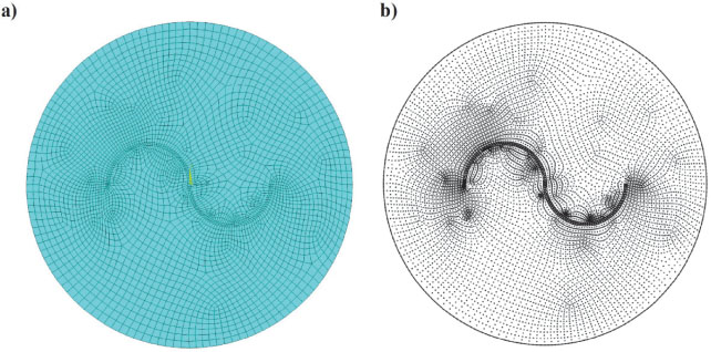
Figure 05: The finite element discretization of the circular domain with curved line heat sources: (a) 3463 elements, (b) 10502 nodes.

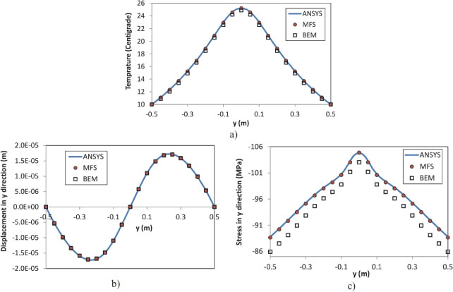
Figure 06: Variations of field variables along the vertical diameter: (a) temperature, (b) displacement in y direction, (c) normal stress in y direction.

The obtained results for field variables along the vertical diameter of the circle are shown in Figure 6. As can be seen, with only 8 source points and without using any internal points, the MFS results are better than the BEM results with the same number of unknowns (8 nodes), and are in a close agreement with the FEM results with a large number of elements. Also, as presented in Section 3.1, it can be seen from the figures that the stress, displacement and temperature have finite values at points exactly on the curved line heat source.

In the second 2D example, a $1\times 1m$ square domain with a large number of circular heat sources is considered. The domain involves 30 circular heat sources in different locations. The radius of each heat source is 0.05 m and the intensity of each heat source is 2500 W/m. The boundary conditions and the layout of the heat sources are shown in Figure 7.

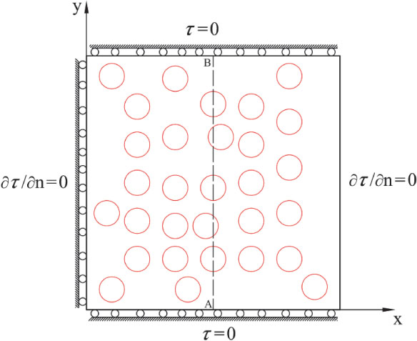
Figure 7: A square with 30 circular heat sources.

In the proposed MFS, each circular heat source is modelled with 4 quadratic segments and 36 collocation points and 36 source points are considered on the main and pseudo boundaries, respectively. The configuration of these points is shown in Figure 8.

The results of the present MFS are compared with those of the FEM. In the FEM, 8524 quadratic elements with 25631 nodes are used and each circular heat source is considered as an area source over a ring with thickness of 0.005 m. The finite element mesh is shown in Figure 9.

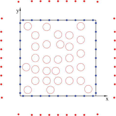
Figure 8: The MFS modelling of the square with 30 circular heat sources.

Figure 9: The finite element discretization of the square domain with 30 circular heat sources: (a) 8524 elements, (b) 25631 nodes.

The obtained results for temperature, displacement and stress variation along the line AB of the square are shown in Figure 10. As can be seen, with only 36 source points and without using any internal points, the MFS results are in very good agreement with the FEM results with a large number of elements and nodes.

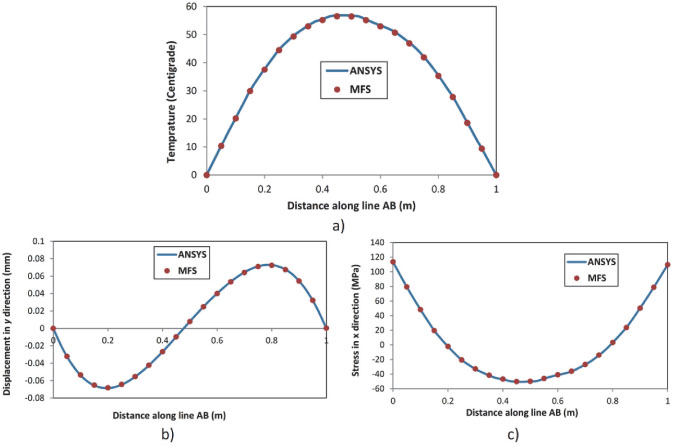
Figure 10: Variations of field variables along the line AB of the square: (a) temperature, (b) vertical displacement and (c) x-direction normal stress.

4.2 Three-dimensional Examples

In the following three-dimensional examples, a spherical domain with radius R $=$ 1 m, and centred at (0, 0, 0) is considered. The surface of the sphere is kept at $\tau =0^{\circ }C$. In the first example, A circular heat source with the radius r $=$ 0.4 m and the centre at ( $-$0.15, 0.2, 0.15) is considered. The plane of the circular heat source is parallel to the $xz$ plane as shown in Figure 11. For better visualization, only a quarter of the spherical domain is shown in Figure 11. The intensity per unit length of the source is considered to be a function of x and the z coordinates with the following form:

$$s=20000\left(1+x^2+z\right){Wm}^{-1}$$

(36)

In the MFS modelling, the circular heat source is divided into 4 quadratic segments. Only 98 source points and 98 collocation points are used. Source points are distributed on surface of a sphere with radius $R^{\prime }=1.4m$.

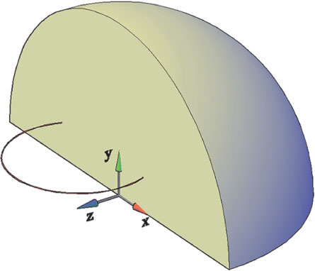
Figure 11: A cut out of the spherical domain including a circular heat source.

The MFS solutions are compared with the FEM solutions. In the FE analysis, the heat source, which is concentrated over a circular ring, should be modelled as a torus with a small minor radius. The major and minor radii of this torus are considered as $r_o=0.4m$ and $r_i=0.02m$, respectively. The torus and a quarter of the spherical domain are shown in Figure 12.

The whole domain is discretized with 40,094 3D quadratic elements and 54,040 nodes. As can be seen in Figure 13, a large number of nodes should be used, especially near the heat source region.

Variations of field variables along the y and z axes are depicted in Figures 14 and 15, respectively. As it can be observed, the MFS results are in a close agreement with the FEM solutions with a note that the modeling of the problem in the proposed MFS is much simpler than that in the FEM.

To verify the accuracy of the proposed formulation for curved surface heat sources, another 3D example is analysed. In this example, the previous sphere with a cylindrical surface heat source is considered. The base of the cylinder is centred at (0, 0, 0). The radius and the height of the cylindrical heat source are 0.2 m and 0.8 m, respectively. The heat source intensity is assumed a function of x, y and z coordinates as follows:

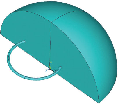
Figure 12: Finite element modelling of the circular heat source by a torus with a small thickness.

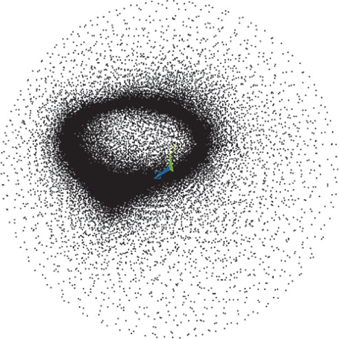
Figure 13: The nodes in the finite element discretization of the sphere with circular heat source.

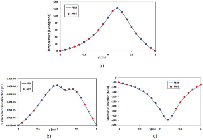
Figure 14: The MFS and FEM results for (a) the temperature (b) horizontal displacement and (c) x-direction normal stress along the y-axis in the sphere with a circular heat source.

$$s=20y\left(1+e^{xz}\right)kW∕m^2$$

(37)

In the MFS modelling, 8 quadrilateral quadratic segments are used for discretization of the cylindrical surface heat source. Pseudo boundary, number of source points and collocation points are the same as the previous example. The results of the proposed MFS are compared with the results obtained by the FEM. In the finite element modelling, the surface heat source is considered as a cylindrical volume heat source with a small thickness of 0.04. The cylindrical volume and a quarter of the spherical domain are shown in the Figure 16.

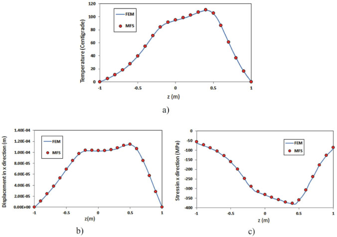
Figure 15: The MFS and FEM results for (a) the temperature (b) horizontal displacement and (c) x-direction normal stress along the z-axis in the sphere with a circular heat source.

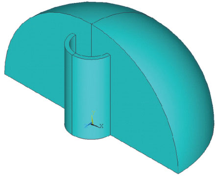
Figure 16: Finite element modelling of the curved surface heat source by a thin-walled cylinder.

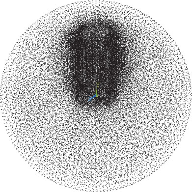
Figure 17: The nodes in the finite element discretization of the sphere with cylindrical heat source.

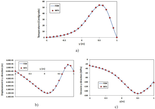
Figure 18: The MFS and FEM results for (a) the temperature (b) vertical displacement and (c) y-direction normal stress along the y-axis in the sphere with a cylindrical heat source.

The total number of 3D quadratic elements is 33448 which include 46376 nodes. The nodal configuraion of the finite element mesh is shown in Figure 17.

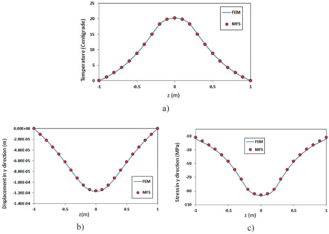
Figure 19: The MFS and FEM results for (a) the temperature (b) vertical displacement and (c) y-direction normal stress along the z-axis in the sphere with a cylindrical heat source.

The variations of field variables along the y and z axes are shown in Figures 18 and 19, respectively. These figures show very good agreement between the proposed MFS results and the FEM solutions. Also, as presented in Section 3.3, it can be seen from Figure 19 that the stress, displacement and temperature have finite values at points exactly on the curved surface heat source.

5 Conclusions

A formulation based on the MFS-MPS was presented for 2D and 3D thermo-mechanical problems involving curved line/surface heat sources. The particular solutions associated with the arbitrary heat sources were presented in simple integral forms. These integrals were evaluated efficiently without considering any internal cells or internal points. Unlike the FEM, modelling of the concentrated heat sources is very simple in the proposed MFS. For reliable FEM modelling, a 2D curved line heat source should be modelled as an area heat source over a narrow region of the domain and 3D curved line/surface heat sources should be modelled as volume heat sources with small thicknesses. The accuracy of the analysis by the FEM depends on the mesh density especially near the concentrated heat source. On the other hand, in the presented MFS, a small number of source and collocation points are sufficient to achieve accurate results. By presenting four examples, the effectiveness and efficiency of the proposed formulation were demonstrated. The obtained results showed that the proposed MFS is very efficient.

References

[1] Chao, C. K., & Tan, C. J. (2000). On the general solutions for annular problems with a point heat source. Journal of Applied Mechanics, 67, 511–518.

[2] Han, J. J., & Hasebe, N. (2002). Green’s functions of point heat source in various thermoelastic boundary value problems. Journal of Thermal Stresses, 25, 153–167.

[3] Rogowski, B. (2016). Green’s function for a multifield material with a heat source. Journal of Theoretical and Applied Mechanics, 54, 743–755.

[4] Le Niliot, C. (1998). The boundary element method for the time-varying strength estimation of point heat sources: application to a two-dimensional diffusion system. Numerical Heat Transfer, part B, 33, 301–321.

[5] Le Niliot, C., Rigollet F., & Petit, D. (2000). An experimental identification of line heat sources in a diffusive system using the boundary element method. International Journal of Heat and Mass Transfer, 43, 2205–2220.

[6] Karami, G., & Hematiyan, M. R. (2000a). Accurate implementation of line and distributed sources in heat conduction problems by the boundary-element method. Numerical Heat Transfer, Part B, 38, 423–447.

[7] Karami, G., & Hematiyan, M. R. (2000b). A boundary element method of inverse non-linear heat conduction analysis with point and line heat sources. International Journal for Numerical Methods in Biomedical Engineering, 16, 191–203.

[8] Shiah, Y. C., Guao, T. L., & Tan, C. L. (2005). Two-dimensional BEM thermoelastic analysis of anisotropic media with concentrated heat sources. CMES Computer Modeling in Engineering and Sciences, 7, 321–338.

[9] Shiah, Y. C., Hwang P. W., & Yang, R. B. (2006). Heat conduction in multiply adjoined anisotropic media with embedded point heat sources. Journal of Heat Transfer, 128, 207–214.

[10] Hematiyan, M. R., Mohammadi, M., & Aliabadi, M. H. (2011). Boundary element analysis of two and three-dimensional thermo-elastic problems with various concentrated heat sources. Journal of Strain Analysis for Engineering Design, 46, 227–242.

[11] Mohammadi, M., Hematiyan, M. R., & Khosravifard, A. (2016). Boundary element analysis of 2D and 3D thermoelastic problems containing curved line heat sources. European Journal of Computational Mechanics, 25, 147–164.

[12] Burgess, G., & Mahajerin, E. (1984). A comparison of the boundary element and superposition methods. Computers & Structures, 19, 697–705.

[13] Mohammadi, M., Hematiyan, M. R., & Shiah, Y. C. (2018). An efficient analysis of steady-state heat conduction involving curved line/surface heat sources in two/three dimensional isotropic media. Journal of Theoretical and Applied Mechanics, 56, 1123–1137.

[14] Mathon, R., & Johnston, R. L. (1977). The approximate solution of elliptic boundary value problems by fundamental solutions. SIAM Journal of Numerical Analysis, 14, 638–650.

[15] Fairweather, G., & Karageorghis, A. (1998). The method of fundamental solutions for elliptic boundary value problems. Advances in Computational Mathematics, 9, 69–95.

[16] Fairweather, G., Karageorghis, A., & Martin, P. A. (2003). The method of fundamental solutions for scattering and radiation problems. Engineering Analysis with Boundary Elements, 27, 759–769.

[17] Karageorghis, A., Lesnic, D., & Marin, L. (2011). A survey of applications of the MFS to inverse problems. Inverse Problems in Science and Engineering, 19, 309–36.

[18] Liu, Q. G., & Šarler, B. (2013). Non-singular method of fundamental solutions for two-dimensional isotropic elasticity problems. Computer Modeling in Engineering and Sciences, 91, 235–266.

[19] Partridge, P. W., Brebbia, C. A., & Wrobel, L. C. (1992). The dual reciprocity boundary element method. Southampton, Computational Mechanics Publications.

[20] Golberg, M. A. (1995). The method of fundamental solutions for Poisson’s equation. Engineering Analysis with Boundary Elements, 16, 205–213.

[21] Medeiros, G. C., Partridge, P. W., & Brand?o, J. O. (2004). The method of fundamental solutions with dual reciprocity for some problems in elasticity. Engineering Analysis with Boundary Elements, 28, 453–461.

[22] Wang, H., & Qin, Q. H. (2008). Meshless approach for thermo-mechanical analysis of functionally graded materials. Engineering Analysis with Boundary Elements, 32, 704–712.

[23] Tsai, C. C. (2009). The method of fundamental solutions with dual reciprocity for three dimensional thermoelasticity under arbitrary forces. Engineering Computations, 26, 229–244.

[24] Poullikkas, A., Karageorghis, A., & Georgiou, G. (1998). The method of fundamental solutions for inhomogeneous elliptic problems. Computational Mechanics, 22, 100–107.

[25] Karageorghis, A., & Smyrlis, Y. S. (2007). Matrix decomposition MFS algorithms for elasticity and thermo-elasticity problems in axisymmetric domains. Journal of Computational and Applied Mathematics, 206, 774–795.

[26] Marin, L., & Karageorghis, A. (2013). The MFS–MPS for two-dimensional steady-state thermoelasticity problems. Engineering Analysis with Boundary Elements, 37, 1004–1020.

[27] Marin, L., Karageorghis, A., & Lesnic, D. (2016). Regularized MFS solution of inverse boundary value problems in three-dimensional steady-state linear thermoelasticity. International Journal of Solids and Structures, 91, 127–142.

[28] Liu, Q. G., & Šarler, B. (2017). A non-singular method of fundamental solutions for two-dimensional steady-state isotropic thermoelasticity problems. Engineering Analysis with Boundary Elements, 75, 89–102.

[29] Becker, A. A. (1992). The Boundary Element Method in Engineering: A Complete Course. McGraw-Hill Book Company.

[30] Stroud, A. H., & Secrest, D. (1966). Gaussian quadrature formulas. New York, Prentice-Hall.

[31] Telles, J. C. F. (1987). A self-adaptive coordinate transformation for efficient numerical evaluation of general boundary element integrals. International Journal for Numerical Methods in Engineering, 24, 959–973.

[32] Aliabadi, M. H. (2002). The boundary element method, applications in solids and structures (Vol.2). Chichester: John Wiley & Sons.

[33] Hematiyan, M. R., Haghighi, A., & Khosravifard, A. (2018). A two-constrained method for appropriate determination of the configuration of source and collocation points in the method of fundamental solutions for 2D Laplace equation. Advances in Applied Mathematics and Mechanics, 10, 554–580.

Biographies

M. Mohammadi received his Ph.D. in Mechanical Engineering from Shiraz University, Shiraz, Iran in 2010. His thesis was about the boundary element analysis of thermo-mechanical problems. He is currently an Assistant Professor at the Department of Mechanical Engineering of Islamic Azad University, Shiraz branch, where he has been a faculty member since 2010. His research interests include computational mechanics, boundary element method, method of fundamental solutions, elasticity and thermo-elasticity.

M. R. Hematiyan received his Ph.D. in Mechanical Engineering from Shiraz University, Iran in 2000. He is currently a full professor at the Department of Mechanical Engineering of Shiraz University, where he has been a faculty member since 2001. He has authored more than 75 journal papers and has been supervisor of more than 70 Ph.D. and M.Sc. thesis. His research interests include computational mechanics, inverse problems, finite element and mesh-free methods, boundary element method, elasticity, thermo-elasticity, hyper-elasticity, and visco-elasticity.

A. Khosravifard received his Ph.D. in Mechanical Engineering from Shiraz University, Shiraz, Iran, in 2012. He joined the Department of Solid Mechanics at School of Mechanical Engineering, Shiraz University as an Assistant Professor, in 2013. He has authored around 50 scientific publications. His areas of expertise include computational mechanics, meshfree methods, fracture mechanics, inverse methods, solidification and moving boundary problems, static and dynamic analysis of structures, and functionally graded materials.

European Journal of Computational Mechanics, Vol. 28 1&2, 51–80.
doi: 10.13052/ejcm1958-5829.28123
© 2019 River Publishers

Abstract

1 Introduction

2 Basic Equations and Formulation

3 Formulations for Heat Sources Concentrated on a Curved Line/Surface

3.1 Curved Line Heat Source in Two-dimensional Problems

3.2 Curved Line Heat Source in 3D Problems

3.3 Curved Surface Heat Source in 3D Problems

4 Numerical Examples

4.1 Two-dimensional Examples

4.2 Three-dimensional Examples

5 Conclusions

References

Biographies