Hypersingular Boundary Integral Equation for Harmonic Acoustic Problems in 2.5D Domains with Moving Sources
J. Pizarro-Ruiz, Esther Puertas García* and Rafael Gallego
Departamento de Mecánica de Estructuras e Ingeniería Hidráulica, ETS de
Ingenieros de Caminos, Canales y Puertos, Universidad de Granada, Avenida
Fuentenueva s/n, 18002 Granada, Spain
E-mail: epuertas@ugr.es
*Corresponding Author
Received 05 March 2019; Accepted 03 July 2019;
Publication 05 August 2019
Abstract
A challenge faced when modeling coincident boundaries by the Boundary Element Method, is to obtain an accurate approximation of integrals which have singular and/or hypersingular kernels. In this paper, we apply a procedure based on regularization of the kernels to compute singular and hypersingular integrals for time harmonic wave problems in two and a half dimensional (2.5D) domains. For this purpose, the Fundamental Solution is described and the study of the terms that arise taking its limit as is carried out. These terms lead to Singular Boundary Integral Equation (SBIE) and Hypersingular Boundary Integral Equation (HBIE). Regular terms of SBIE and HBIE are integrated by applying numerical quadratures, whereas singular and hypersingular terms are calculated analytically. Working in 2.5D domains make it easier to compute moving sources. A procedure, which leads to a simple change of the frequency of the problem, is described in this paper. Numerical results are presented for acoustic problems with coincident boundaries to demonstrate the accuracy of the proposed formulation.
Keywords: BEM, 2.5D, Hypersingular, Acoustic barriers, Coincident Boundaries, Moving Sources, Helmholtz Equation
1 Introduction
There is no doubt that noise pollution is a serious problem in our society. There are many diseases related to the increment of noise near housings [1]. Acoustic barriers are built to reduce or eliminate rail or car traffic noise. Thus, a good tool to estimate it is needed, in order to improve life quality in the cities. Many authors have studied the modeling of acoustic barriers; Finite Differences Method and Finite Element Method (FEM) were often used on this purpose. When Boundary Element Method [2, 3] appeared, new ways to address the problem were developed. A great advantage of this method when compared to FEM is that an infinite domain can be modeled easily, satisfying the far-field conditions, without having to increase the number of elements. This is why BEM is used in this paper to model sound propagation in air.
Acoustic barriers, which pursue the aim of restricting noise levels, are often modeled as an infinitely thin domain [4]. In BEM formulation, this would lead to a pair of infinitely close boundaries which are called Coincident Boundaries. Although BEM shows strong performance in wave propagation analysis problems, modeling these special boundaries using BEM leads to the integration of functions with hypersingular kernels, which are not easy to compute. For this purpose, many authors have proposed different techniques to face this problem. Gray [5] uses a linear function to represent the integrand function over the domain; [6] presents a regularization of the kernels by using simple solutions; [7] use polar transformation and Lauren expansion series are used to derive the hypersingular integral; [8] employ image source technique to avoid hypersingular terms. In this work, we apply the regularization procedure presented by [9] for the purpose of computing singular and hypersingular integrals in two and a half dimensional (2.5D) domains.
Another important issue when facing traffic noise calculations is estimating the effect of a moving emitting source. As traffic is composed by different moving sources such as cars or buses, it is needed to study the impact of their speed on the modeling problem. Some authors propose different ways to study this issue. Andersen and Nielsen [10] study the ground noise produced by a train load using moving coordinates. Tadeu et al. [11] use a 3D incident field in order to calculate sound absorption when the source is moving at constant speed in 2.5D problems. An interesting result is suggested by [12], who use source loads activated in different time-steps to simulate a moving load. In this paper, we propose a procedure to convert the moving-source problem into a fixed source problem which could be used in 2.5D domains problems. Although this work shows the formulation for the particular case of acoustic barriers, this procedure can also be applied to any wave propagation problem in 2.5D with coincident boundaries (such as antiplane shear problems near cracks) by just changing the meaning of the variables and constants, provided that the problem follows Helmholtz equation.
2 Boundary Element Formulation
The scalar Helmholtz equation can be written as:
| (1) |
In the particular case of 3D acoustics, is the wave propagation speed inside the fluid, are the external forces, is the fluid pressure and . For time harmonic problems, a Fourier Transform along time-axis can be done to convert the problem from time-domain to frequency-domain. Also, if the geometry of the acoustic domain does not vary along -coordinate, a parameter called wave number can be defined, and making another Fourier Transform along -axis would lead to:
| (2) |
This formulation express the solution of Eq:Helmoltz as an infinite sum of waves with different and . Substitution of (2) into (1), assuming there is no external forces () and with some rearrangement, gives the homogeneous Helmoltz equation in 2.5D:
| (3) |
where and . Let be the 2D boundary of the acoustic domain, be a point over , and let be the collocation point of the fundamental solution of (3) standard boundary integral equation (PBIES) of this equation is:
| (4) |
where is the pressure gradient and is the so called “free term”. and are, respectively, the fundamental solutions for the pressure and the pressure gradient:
where and are Hankel functions of second kind and , the Euclidean distance between the point over the domain and the collocation point :
When there is a rigid barrier inside the domain, its boundary can be expressed as a sum of three parts: the exterior boundary and two coincident boundaries ( and ), one for each face of the barrier [13]. As shown in Figure 1, both and are infinitely close, so if is over one of these boundaries, Eq:PBIES leads to an incompatible system of equations. Let be the normal vector of , then, would be the normal vector of boundary . Thus, with some rearrangement, (4) when is over the barrier is:
| (5) |

Figure 1: Example of a domain with a barrier on it inside. Both faces of the barrier are infinitely close to each other ().
Calling and , gives (5) as:
| (6) |
Using (6), instead of two separate equations for each face of the barrier, make the system of equation indeterminate. Thus, in order to have a determinate system, a new equation is needed. For this purpose, (6) can be derived with respect to over the direction defined by the vector , which is the normal vector in the collocation point. This leads to:
| (7) |
where
| (8a) |
| (8b) |
and the summation convention for repeated indices is adopted. Equation (6) is called Gradient Boundary Integral Equation (QBIES). The main disadvantage of using QBIES formulation is that it yields integrals with hypersingular kernels. A way to avoid this obstacle is proceed as follows. First, (8a) has to be expressed as a combination of Hankel functions:
| (9) |
where . In order to get non-regular terms of (9), Lauren expansion of its Hankel functions has been done. Two non-regular terms have been obtained:
-
which is hypersingular
- which is singular
Both terms are regularized and integrated following the procedure described in [9]. The same procedure has to be done with (8b). Expressing it as a combination of Hankel functions:
| (10) |
In this case, after making a Lauren expansion of this function, all resultant terms are regular. Thus, no special integration is needed and integrals can be calculated numerically.
3 Numerical Examples
In order to show the accuracy of the previous method, we have calculated a theoretical example. Let us consider a 2.5D domain where there is a rigid barrier. Assuming , and given boundary conditions expressed in Figure 2, and all units according to the International System of Units; we are going to compare results obtained after an analysis with both PBIES and QBIES. In the case of PBIES, the barrier can be modeled as an elliptical boundary where its semi-minor axis . On the other hand, for a QBIES formulation, the barrier will be modeled as a pair of coincident boundaries, as shown previously.
After both analysis, we show the results for the base boundary (), and for the barrier in Figure 3. Also, we have calculated the pressure in some internal points (Figure 4).
As we can see in Figures (3–4), as long as the semi-minor axis tends to 0, PBIES results tend to the solution with QBIES formulation. When is too small, the system of equations obtained with PBIES formulation is not consistent. In contrast, coincident boundaries formulation has a better performance, as the barrier is already infinitely thin. Thus, the accuracy of the results is better.
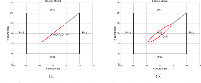
Figure 2: (a) Model with a pair of coincident boundaries and its boundary conditions. (b) Model with elliptical barrier. Crosses are internal points, where P will be calculate.
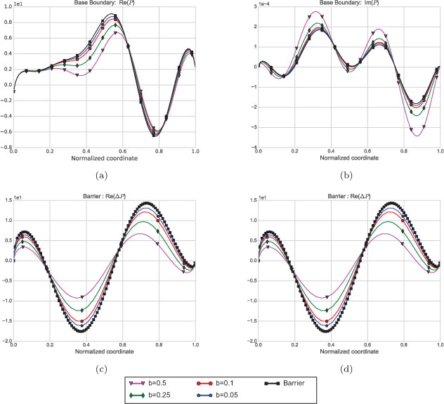
Figure 3: Comparison between calculated with QBIES, and PBIES for different values. (a) and (b) show real part and imaginary part respectively, of in base boundary. (c) and (d) show real part and imaginary part respectively, of in the barrier. Dimension of both boundaries have been normalized from 0 to 1.
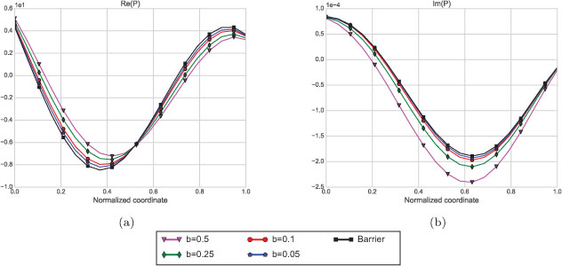
Figure 4: Comparison between obtained in internal points calculated with QBIES, and PBIES for different values. Distance from the barrier has been normalized from 0 on the left and down to 1 on the right and up. (a) shows the real part and (b) shows the imaginary part.
4 Moving Sources
One of the main advantages of working in 2.5D domains is when applied loads are moving constantly along one coordinate. Traffic noise problems can belong to these kind of situations. Let us have a 3D acoustic domain with an invariant geometry along direction, and a point load moving with constant speed along direction. If we call and the applied moving load in 3D domain and in 2.5D domain, respectively; and we follow the procedure described in Section 2 to work in and domain:
| (11) |
making the appropriate change of variables in previous equation:
| (12) |
where is the solution for a fixed load (Section 2) with frequency. Thus, being , Helmholtz differential equation results:
As a consequence of the previous demonstration, the moving source problem, when working in 2.5D domains, can be solved using the fixed source formulation (Section 2) by just changing for . In order to illustrate how to proceed when a moving source is applied to a 3D domain, the following example is given. Let us have a street where an acoustic barrier separates a building from a highway as shown in Figure 5(a). Let us consider a given source of frequency moving at constant speed and three observation points represented in Figure 5(b). Let also consider there is no air flux through the ground and the barrier, thus boundary conditions in both boundaries would be .
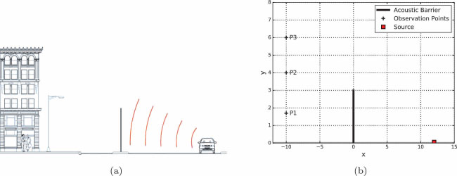
Figure 5: (a) Example problem. (b) Diagram of the problem in a 2.5D dimension model, crosses are observation points where the solution will be computed.
Using the formulation described in precedent sections, we are going to calculate the noise reduction resulting from the insertion of an acoustic barrier between the highway and the building for several values of : [km/h]. Insertion loss (IL) [4] is determined as follows:
| (13) |
where is the mean squared pressure without the barrier and is the mean squared pressure with the barrier. A general solution of the problem could be computed by just varying and . Figure 6(a) represents this solution at the first observation point (height m) when the frequency Hz. For any given , the resultant would be the general solution calculated over the equation line , as showed in Figure 6(b). Thus, following this procedure, we can obtain the solution at any given frequency for any value of by just evaluating over its equation line.
Figures 7–9 show the resultant when the solution is evaluated at the three observation points at a frequency of 650 Hz. As can be seen, for the same frequency of the source, different values of the speed lead to different solutions of the problem.
As a final result, an Inverse Fourier Transform of along dimension is represented when the speed is [km/h] and the frequency is 450 Hz (Figure 10). We have compute the solution for 256 points varying from 6 to 6 rad/m.
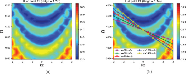
Figure 6: (a) General solution of the problem ( rad/s and rad/m). Abscissa axis represent , ordinate axis is and color scale is the insertion loss. Image (b) shows different lines, one for each value of , where is evaluated.
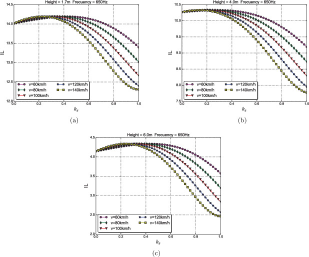
Figure 7: evaluated at observation points when the frequency of the source is Hz.
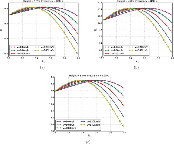
Figure 8: evaluated at observation points when the frequency of the source is Hz.
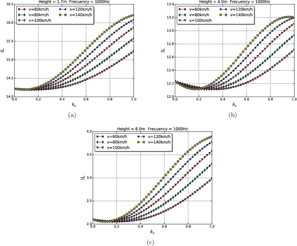
Figure 9: evaluated at observation points when the frequency of the source is Hz.
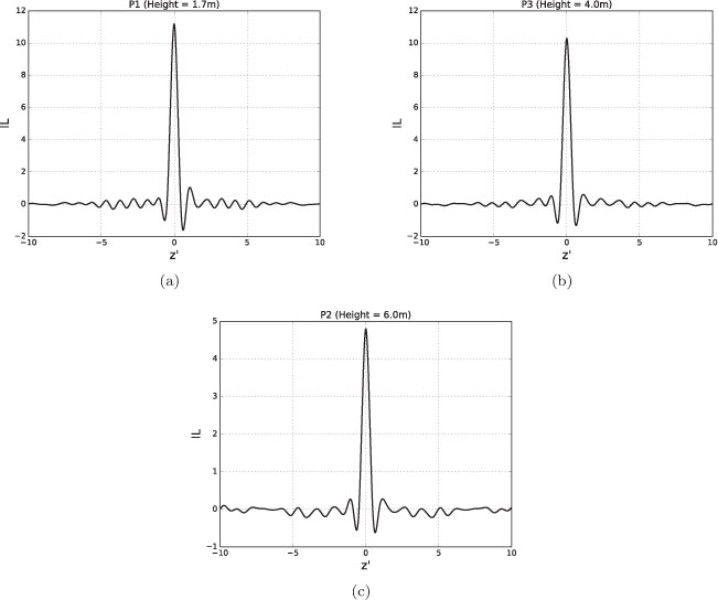
Figure 10: Results in three observation points (P1, P2, P3) on a 3D geometry domain and frequency domain.
5 Conclusions
In this paper, we propose a way to apply the Boundary Element Method to acoustic problems where a barrier is placed to reduce traffic noise. Acoustic barriers are modeled as a pair of infinitely close boundaries that produce integrals whose kernels are hypersingular. The suggested way to solve this kind of integrals is by making a regularization of their kernels, which makes it possible to compute them by numerical integration.
Traffic sound sources, such as cars or trains, can be modeled as point loads moving along one direction parallel to the barrier. Transforming the problem dimension from 3D to 2.5D has the great advantage of allowing the use of a fixed source formulation with a simple modification of the frequency. An example problem has been solved in order to present the method, whose results can be seen in Figures 7–9. These figures show the effect of the speed on insertion loss of the acoustic barrier.
References
[1] Stansfeld, S. A. and Matheson, M. P. (2003). Noise pollution: Non-auditory effects on health. British Medical Bulletin, 68, 243–257.
[2] Brebbia, C. and Domínguez, J. (1992). Boundary Elements: AnIntroductory Course. Ashurst, Southampton: Wit Press.
[3] Domínguez, J. (1993). Boundary Elements in Dynamics. Ashurst, Southampton: Wit Press.
[4] Maeso, O. and Aznárez, J. J. (2005). Estrategias para la reducción del impacto acústico en el entorno de carreteras. Una aplicación del método de los elementos de contorno. Servicio de Reprografía de la U.L.P.G.C.
[5] Gray, L. (1991). Evaluation of hypersingular integrals in the boundary element method. Mathematical and Computer Modelling, 15(3–5), 165–174.
[6] Rudolphi, T. (1991). The use of simple solutions in the regularization of hypersingular boundary integral equations. Mathematical and ComputerModelling, 15(3), 269–278.
[7] Guiggiani, M., Krishnasamy, G., Rudolphi, T. J. and Rizzo, F. J.(1992). A General Algorithm for the Numerical Solution of Hypersingular Boundary Integral Equations. Journal of Applied Mechanics, 59(3), 604.
[8] Tadeu, A., António, J., Amado-Mendes, P. and Godinho, L. (2007).Sound pressure level attenuation provided by thin rigid screens coupled to tall buildings. Journal of Sound and Vibration, 304(3–5), 479–496.
[9] Sáez, A., Gallego, R. and Dominguez, J. (1995, may). Hypersingular quarterpoint boundary elements for crack problems. International Journalfor Numerical Methods in Engineering, 38(10), 1681–1701.
[10] Andersen, L. and Nielsen, S. R. (2005). Reduction of ground vibration by means of barriers or soil improvement along a railway track. SoilDynamics and Earthquake Engineering, 25(7–10), 701–716.
[11] Tadeu, A., António, J., Godinho, L. and Amado-Mendes, P. (2012).Simulation of sound absorption in 2D thin elements using a coupled BEM/TBEM formulation in the presence of 3D sources. InternationalJournal for Housing Science and Its Applications, 36(4), 189–198.
[12] Lefévre, F. and Le Niliot, C. (2002). The BEM for point heat source estimation: Application to multiple static sources and moving sources.International Journal of Thermal Sciences, 41(6), 536–545.
[13] Bordón, J. D., Aznárez, J. J. and Maeso, O. (2014). A 2DBEM-FEM approach for time harmonic fuid-structure interaction analysis of thin elastic bodies. Engineering Analysis with Boundary Elements, 43, 19–29.
Biographies
J. Pizarro-Ruiz is a Ph.D student at the University of Granada since 2018. He attended the University of Granada, Spain, where he received his bachelor degree in Civil Engineering in 2016. He continued his studies at this University and obtained Master degree in Structures. Joaquín is working on his doctorate in Civil Engineering at University of Granada. His Ph.D work studies vibrations propagation modeling with Boundary Elements Method in poroelastic soils and spectral analysis of superficial waves, in order to obtain the properties of soils under the sea level.
Esther Puertas García is permanent lecturer at the University of Granada. She received her Bachelor and Master degrees in Civil Engineering at the University of Granada, and PhD degrees in Civil Engineering from the University of Granada in 2014. She has an extensive teaching, research and professional experience in the Mechanics of Continuous Media and Theory of Structures topics. Her research work concerns the development of computational toolkits for continuum media dynamics. She belongs to the Research Group of Mechanics of Solids and Structures. Her lines of work are based on the study of Integral Equations Methods for advanced applications in Solid Mechanics. She has developed techniques for the analysis of wave propagation problems in two and a half domains.
Rafael Gallego is full professor at the University of Granada since 1995. He received his Bachelor and Master degrees in Structural and Mechanical Engineering at the University of Sevilla (1987) and got his PhD at the same University in 1990; he was granted a Fulbright postdoctoral scholarship (1990–92) at the Brown University. Among other academic posts, he has been chairman of the Department of Structural and Hydraulic Engineering at the University of Granada since 2000 to 2008 and since 2016 to date. His research work has focused in developing computational models based on Boundary Integral Equations for solid mechanics problem, mainly related to wave propagation in solids, dynamic fracture mechanics and dynamic soil-structure interaction, including resolution of inverse problems to match computational results and experimental ones.
European Journal of Computational Mechanics, Vol. 28 1&2, 81-96.
doi: 10.13052/ejcm1958-5829.28124
© 2019 River Publishers