Numerical Simulation Using a Modified Solver within OpenFOAM for Compressible Viscous Flows

Valiyollah Ghazanfari¹, Ali Akbar Salehi², Alireza Keshtkar^1,*, Mohammad Mahdi Shadman³ and Mohammad Hossein Askari³

¹Materials and Nuclear Fuel Research School, Nuclear Science and Technology Research Institute, AEOI, Tehran, Iran

²Department of Energy Engineering, Sharif University of Technology, Tehran, Iran

³Advanced Technology Company of Iran, AEOI, Tehran, Iran

Email: akeshtkar@aeoi.org.ir

* Corresponding Author

Received 06 September 2019; Accepted 06 December 2019; Publication 28 February 2020

Abstract

In this work, we attempted to develop an Implicit Coupled Density-Based (ICDB) solver using LU-SGS algorithm based on the AUSM⁺ up scheme in OpenFOAM. Then sonicFoam solver was modified to include viscous dissipation in order to improve its capability to capture shock wave and aerothermal variables. The details of the ICDB solver as well as key implementation details of the viscous dissipation to energy equation were introduced. Finally, two benchmark tests of hypersonic airflow over a flat plate and a 2-D cylinder were simulated to show the accuracy of ICDB solver. To verify and validate the ICDB solver, the obtained results were compared with other published experimental data. It was revealed that ICDB solver has good agreement with the experimental data. So it can be used as reference in other studies. It was also observed that ICDB solver enjoy advantages such as high resolution for contact discontinuity and low computational time. Moreover, to investigate the performance of modified sonicFoam, a case study of airflow over the prism was considered. Then the results of the modified sonicFoam were compared with the ICDB, rhoCentralFoam and sonicFoam solvers. The results showed that the modified sonicFoam solver possesses higher accuracy and lower computational time in comparison with the sonicFoam and rhoCentralFoam solvers, respectively.

Keywords: OpenFOAM, density-based, AUSM⁺ up, sonicFoam, implicit.

1 Introduction

In a viscous fluid flow, the viscosity of the fluid dissipates the fluid’s mechanical energy into the internal energy; this process is partially irreversible. Viscous dissipation usually refers to the work done by the flow against the viscous stresses [1]. It has been studied by many researchers [2–5].

Stewartson studied the compressible boundary-layer characteristics using analytical and numerical methods, and presented the effects of viscosity variations with temperature [6]. Nepal et al. investigated the flow and the effect of viscous dissipation, as well as the heat transfer characteristics of compressible boundary-layer flow passing through a heated cylinder. For different Mach numbers and surface temperatures, the numerical solutions demonstrated how the local shear stress and the rate of heat transfer at the surface of the cylinder were affected by these parameters [7].

There are many procedures for numerical simulation: explicit or implicit and coupled or segregated schemes.

Explicit and implicit schemes are usually used in time discretization in Computational Fluid Dynamic (CFD). The computational cost of implicit scheme is more than that of explicit scheme because it needs to solve a linear system of equations at each time step. However, since explicit scheme uses only the previous flow field information while implicit scheme uses the current flow field information. In addition, the solution in implicit scheme is, generally, more stable [8].

In coupled method, the dependent equations are solved simultaneously. This method is more efficient; however, because of its complexity, it needs higher memory requirements [11]. Commercial CFD packages such as Fluent are quite convenient and efficient; they use the fully implicit coupled method but provide solutions only for general situations considered by the designers [12]. The limited programming interface in Fluent makes it difficult to use these packages to implement new models for specific needs. In contrast, OpenFOAM is a free-source CFD package that provides both tutorials and the C++ source code. The existing calculation modules can be used similar to commercial CFD software. Also the C++ source code can be modified for different purposes [13–16]. In the official version of OpenFOAM, an explicit segregated density-based compressible solver, called rhoCentralFoam, has been developed that uses the central-upwind schemes of Kruganov and Tadmor to capture the shocks.

The discrete details of rhoCentralFoam are shown in Ref. [17]. The number of functions of density-based solvers and their efficiency are relatively lower in the official version of OpenFOAM. The DensityBasedTurbo solver has been developed by the extended version of OpenFOAM. The well-known Godunov convective discrete schemes (e.g. AUSM family and Roe) are used in this solver [16–18], as well as in commercial CFD codes (Fluent, Fastran and CFX) [21–23].

The present work aimed at (i) development of Implicit Coupled Density-Based (ICDB) solver using AUSM⁺ up scheme in OpenFOAM framework, (ii) proposing a new modified sonicFoam (i.e. adding the viscous dissipation to the energy equation), and (iii) verification and validation of ICDB by comparing with Chun’s findings and other experimental data. To this end, three test cases are considered: (a) hypersonic airflow over an adiabatic flat plate, (b) hypersonic airflow over an isothermal cylinder, and (c) supersonic airflow over an adiabatic prism. In the prism case, the results of ICDB, modified sonicFoam, rhoCentralFoam, and sonicFoam solvers are compared. The present work ultimately aims to show the performance of the above mentioned solvers in OpenFOAM for compressible flows.

2 Governing Equations

The governing equations for the conservation of mass, momentum and energy are as follows, respectively [24]:

$$\frac{\partial \rho }{\partial t}+\nabla \cdot \mathrm{<mo\; stretchy="false">(</mo>}\rho V\mathrm{<mo\; stretchy="false">)</mo><mo>=</mo>0,}$$

(1)

$$\frac{\partial \mathrm{<mo\; stretchy="false">(</mo>}\rho V\mathrm{<mo\; stretchy="false">)</mo>}}{\partial t}+\nabla \cdot \mathrm{<mo\; stretchy="false">(</mo>}\rho VV\mathrm{<mo\; stretchy="false">)</mo><mo>=</mo>}-\nabla p+\nabla \cdot \tau \mathrm{,}$$

(2)

$$\frac{\partial \mathrm{<mo\; stretchy="false">(</mo>}\rho e\mathrm{<mo\; stretchy="false">)</mo>}}{\partial t}+\nabla \cdot \mathrm{<mo\; stretchy="false">(</mo>}\rho Ve\mathrm{<mo\; stretchy="false">)</mo><mo>=</mo>}-\nabla \cdot \mathrm{<mo\; stretchy="false">(</mo>}k\nabla T\mathrm{<mo\; stretchy="false">)</mo>}-\nabla \cdot \mathrm{<mo\; stretchy="false">(</mo>}pV\mathrm{<mo\; stretchy="false">)</mo>}+\nabla \cdot \mathrm{<mo\; stretchy="false">(</mo>}\tau \cdot V\mathrm{<mo\; stretchy="false">)</mo>}$$

(3)

where, ρ is the density, V is the velocity vector, p is the pressure, τ is the stress tensor, and e is the specific total energy. The equation of state for ideal gas is $p\mathrm{<mo>/</mo>}\rho \mathrm{<mo>=</mo>}\frac{R}{M}T$, in which R is the universal gas constant, M is the molar mass of the considered gas, and T is the temperature.

For a Newtonian fluid, the stress tensor is a linear function of the strain rate:

$$\tau \mathrm{<mo>=</mo>}\mu \mathrm{<mo\; stretchy="false">[</mo>}\nabla V+{\mathrm{<mo\; stretchy="false">(</mo>}\nabla V\mathrm{<mo\; stretchy="false">)</mo>}}^T\mathrm{<mo\; stretchy="false">]</mo>}+\lambda \mathrm{<mo\; stretchy="false">(</mo>}\nabla \cdot V\mathrm{<mo\; stretchy="false">)</mo>}I$$

(4)

where, μ is the molecular coefficient of viscosity, λ is the bulk coefficient of viscosity, usually set equal to −(2/3)μ (λ = −(2/3)μ), T refers to the transpose of ∇V, and I is the unit or identity tensor.

The divergence of the stress tensor is a vector that can be expressed as:

$$\begin{array}{l}\nabla \cdot \tau \mathrm{<mo>=</mo>}\nabla \cdot \mathrm{<mo\; stretchy="false">[</mo>}\mu \mathrm{<mo\; stretchy="false">[</mo>}\nabla V+{\mathrm{<mo\; stretchy="false">(</mo>}\nabla V\mathrm{<mo\; stretchy="false">)</mo>}}^T\mathrm{<mo\; stretchy="false">]</mo><mo\; stretchy="false">]</mo>}+\nabla \cdot \mathrm{<mo\; stretchy="false">(</mo>}\lambda \mathrm{<mo\; stretchy="false">(</mo>}\nabla \cdot V\mathrm{<mo\; stretchy="false">)</mo><mo\; stretchy="false">)</mo>}\hfill \\ \mathrm{<mo>=</mo>}\left[\begin{array}{l}\frac{\partial }{\partial x}\left[2\mu \frac{\partial u}{\partial x}+\lambda \left(\nabla \cdot v\right)\right]+\frac{\partial }{\partial y}\left[\mu \left(\frac{\partial v}{\partial x}+\frac{\partial u}{\partial y}\right)\right]\hfill \\ +\frac{\partial }{\partial z}\left[\mu \left(\frac{\partial u}{\partial z}+\frac{\partial w}{\partial x}\right)\right]\hfill \\ \frac{\partial }{\partial x}\left[\mu \left(\frac{\partial v}{\partial x}+\frac{\partial u}{\partial y}\right)\right]+\frac{\partial }{\partial y}\left[2\mu \frac{\partial v}{\partial y}+\lambda \left(\nabla \cdot v\right)\right]\hfill \\ +\frac{\partial }{\partial z}\left[\mu \left(\frac{\partial w}{\partial y}+\frac{\partial v}{\partial z}\right)\right]\hfill \\ \frac{\partial }{\partial x}\left[\mu \left(\frac{\partial u}{\partial z}+\frac{\partial w}{\partial x}\right)\right]+\frac{\partial }{\partial y}\left[\mu \left(\frac{\partial w}{\partial y}+\frac{\partial v}{\partial z}\right)\right]\hfill \\ +\frac{\partial }{\partial z}\left[2\mu \frac{\partial w}{\partial z}+\lambda \left(\nabla \cdot v\right)\right]\hfill \end{array}\right]\hfill \end{array}$$

(5)

For modeling the turbulent flow, the standard k−ε model is used.

3 Numerical Schemes

The numerical solution of compressible flow equations can be performed using two different approaches (pressure-based and density-based). In Open-FOAM, both approaches are implemented. RhoCentralFoam is a density-based solver and sonicFoam is a pressure-based solver. Almost all solvers of OpenFOAM can solve the continuity, momentum and energy equations by using a segregated method, sequentially.

3.1 rhoCentralFoam Solver

rhoCentralFoam is an explicit segregated density-based solver in OpenFOAM framework. In rhoCentralFoam, the continuity, momentum and energy equations are discretized separately to obtain three linear systems. These systems are independent, and can be solved separately. The continuity and momentum equations are solved in two steps. For this purpose, the inviscid part of the momentum equation is calculated explicitly and its values are updated. Then the viscous part is added primarily. Next, the energy equation is solved explicitly without the diffusive flux of heat, which is later added when the updated temperature is calculated. The actual inviscid equations are then corrected implicitly by associating the diffusion terms. In rhoCentralFoam, the required flux interpolations are performed using the second-order semi-discrete, non-staggered schemes of Kurganov and Tadmor (KT) [25], and Kurganov, Noelle, and Petrova (KNP) [26]. As a limitation, the Kurganov-Tadmor’s scheme needs to keep the acoustic Courant number less than 1/2 [27]. The main procedure of rhoCentralFoam, which is a part of code in rhoCentralFoam solver written in C++ language is shown in Figure 1.

3.2 sonicFoam Solver

sonicFoam is a semi-implicit segregated pressure-based solver. The method, known as PISO (Pressure Implicit with Splitting of Operators), uses the pressure and velocity as dependent variables. The required pressure equation to be used in sonicFoam may be derived from the differential form of the momentum and continuity equations. The main feature of this technique is splitting of the solution process into a series of steps where the operations on pressure are decoupled from those on velocity [26]. The two key differences between sonicFoam and rhoCentralFoam solvers are the use of pressure and velocity as dependent variables through the PISO method in sonicFoam, and the use of an alternative approach to Riemann solvers, based on central-upwind schemes in rhoCentralFoam. The main procedure of sonicFoam, which is a part of code in sonicFoam solver written in C++ language is shown in Figure 2.

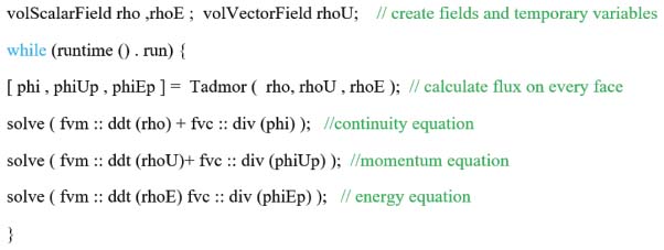
Figure 1 The procedure of rhoCentralFoam.

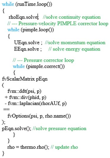
Figure 2 The procedure of sonicFoam.

3.3 Modified sonicFoam Solver

The solution of the energy equation is included in several solvers of Open-FOAM. The energy equation in sonicFoam solver is implemented in the form of total energy expressed in Equation (3), without the mechanical sources ∇ · (τ · V):

$$\nabla \cdot \mathrm{<mo\; stretchy="false">(</mo>}\tau \cdot V\mathrm{<mo\; stretchy="false">)</mo><mo>=</mo><mo\; stretchy="false">(</mo>}\nabla \cdot \tau \mathrm{<mo\; stretchy="false">)</mo>}\cdot V+\tau \mathrm{<mo>:</mo>}\nabla V$$

(6)

where, τ: ∇V represents the conversion of mechanical power into internal energy, and thus, the random motion of particles, and (∇ · τ) · V shows a mechanical power due to the bulk motion of particles. The viscous dissipation rate is:

$$\Phi \mathrm{<mo>=</mo>}\tau \mathrm{<mo>:</mo><mi>\; </mi>}\nabla V\mathrm{<mo>=</mo>}\left(-\frac{2}{3}\mu \nabla \cdot V+\mu \mathrm{<mo\; stretchy="false">[</mo>}\nabla V+{\mathrm{<mo\; stretchy="false">(</mo>}\nabla V\mathrm{<mo\; stretchy="false">)</mo>}}^T\mathrm{<mo\; stretchy="false">]</mo>}\right)\mathrm{<mo>:</mo><mi>\; </mi>}\nabla V\mathrm{.}$$

(7)

In the present study, the mechanical source term was added to the energy equation of sonicFoam solver; we named it “modified sonicFoam”. The C++ programming language was used for this purpose in accordance with the programming structure in OpenFOAM.

This term is calculated by calling devRhoReff()&U. In the modified sonicFoam solver, the energy equation is implemented as follows:

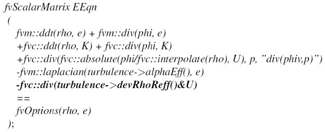
Where, ∇ · τ is used to define the details of ∇ · (τ · V), (turbulence-> divDevRhoReff(U)). The value of (divDevRhoReff(U)) can be shown as:

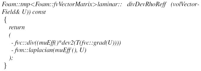
Thus, ∇ · (τ · V) is calculated using (divDevRhoReff()&U).

The purpose of adding an extra source term to sonicFoam is to increase the capability of this solver to analysis the effect of viscous dissipation. Review of other studies shows viscous dissipation has special importance in compressible flows so it is necessary to develop sonicFoam in order to investigating the effect of viscous dissipation.

3.4 ICDB (Implicit Coupled Density-Based) Solver

Computational fluid dynamics codes are becoming a promising tool for regular and routine use in engineering. Hence, more careful attention must be paid for developing a numerical scheme that is reliable for a wide range of applications like physical modeling [29]. One of the important extensions is to allow the application of the existing compressible flow codes to reliably predict low and high speed flows.

Flux difference splitting (FDS) schemes such as the Roe scheme [30] have very high resolution for both contact discontinuity and boundary layer in compressible flows. Flux vector splitting (FVS) schemes have much better robustness in capturing strong discontinuities; however, they have a large numerical dissipation on contact discontinuities and in boundary layers. The AUSM family schemes enjoy the advantages of both FDS and FVS schemes like high resolution for contact discontinuity, low numerical dissipation, and high computational efficiency [19].

In simulation of gas centrifuge, there is a wide range of Mach numbers such that it is low near the axis and high near the wall of the rotor. The objective of the present study is to develop a new scheme that is uniformly valid for all speed regimes.

A new version of the AUSM-family schemes, called AUSM⁺ up based on the low Mach number asymptotic analysis, is described in Liou’s study [29]. It has been demonstrated to be reliable and effective not only for low Mach numbers, but also for all speed regimes, as well as for a wide variety of flow problems over different geometries and grids [29]. In this scheme, central and upwind interpolations are used for subsonic and supersonic flows, respectively [31]. The equations related to Roe and AUSM⁺ up schemes are found in Refs. [29, 30].

In this part, the characteristics of ICDB solver are explained.

The general conservation equations in steady state is as below:

$$\nabla \cdot \mathrm{<mo\; stretchy="false">(</mo>}{\overrightarrow{F}}_c-{\overrightarrow{F}}_v\mathrm{<mo\; stretchy="false">)</mo><mo>=</mo>0}$$

(8)

where, ${\overrightarrow{F}}_c$ and ${\overrightarrow{F}}_v$ are the vectors of the convective and viscous fluxes, respectively, which can be expressed as follows:

$${\overrightarrow{F}}_c\mathrm{<mo>=</mo>}\left[\begin{array}{c}\rho \\ \rho uV+n_{x}p\\ \rho vV+n_{y}p\\ \rho wV+n_{z}p\\ \rho VE\end{array}\right]$$ $${\overrightarrow{F}}_v\mathrm{<mo>=</mo>}\left[\begin{array}{c}0\\ n_x{\tau }_{xx}+n_y{\tau }_{xy}+n_z{\tau }_{xz}\\ n_x{\tau }_{yx}+n_y{\tau }_{yy}+n_z{\tau }_{yz}\\ n_x{\tau }_{zx}+n_y{\tau }_{zy}+n_z{\tau }_{zz}\\ n_x{\theta }_x+n_y{\theta }_y+n_z{\theta }_z\end{array}\right]$$ $$\begin{array}{l}{\theta }_x\mathrm{<mo>=</mo>}u{\tau }_{xx}+v{\tau }_{xy}+w{\tau }_{xz}+u{\dot{q}}_{sx}\hfill \\ {\theta }_y\mathrm{<mo>=</mo>}u{\tau }_{yx}+v{\tau }_{yy}+w{\tau }_{yz}+u{\dot{q}}_{sy}\hfill \\ {\theta }_z\mathrm{<mo>=</mo>}u{\tau }_{zx}+v{\tau }_{zy}+w{\tau }_{zz}+u{\dot{q}}_{sz}\hfill \end{array}$$

In order to solve the conservation equation by implicit coupled method, a system of equations is solved as:

$$\left[\begin{array}{ccc}{a}_{1.1}& \dots & a_{1.n}\\ ⋮& \ddots & ⋮\\ a_{n.1}& \dots & a_{n\mathrm{.}n}\end{array}\right]\left[\begin{array}{c}\rho \\ \rho u\\ \rho v\\ \rho w\\ \rho E\end{array}\right]\mathrm{<mo>=</mo>}\left[\begin{array}{c}{b}_1\\ ⋮\\ b_n\end{array}\right]$$

(9)

The system of equations is solved by the ICDB solver in OpenFOAM framework. The ICDB solver is based on the AUSM⁺ up scheme using LU-SGS (Lower-Upper Symmetric Gauss–Seidel) algorithm and GMRES (Generalized Minimal Residual) method.

Matrix-free LU-SGS implicit scheme is widely used to solve a linear system because of its low numerical complexity and modest memory requirements [10].

Here, the equations system is Ax = b. According to the original theory of LU-SGS scheme, the implicit operator should be divided into the diagonal matrix, D, the lower-diagonal matrix, L, and the upper-diagonal matrix, U, as follows:

$$A\mathrm{<mo>=</mo>}L+D+U\simeq \mathrm{<mo\; stretchy="false">(</mo>}L+D\mathrm{<mo\; stretchy="false">)</mo>}{D}^{-1}\mathrm{<mo\; stretchy="false">(</mo>}D+U\mathrm{<mo\; stretchy="false">)</mo>}$$

(10)

The solving process is divided into two steps: forward sweep and backward sweep, which are directly solved by Equations (11) and (12), respectively:

$$D\Delta x^{\mathrm{<mo>*</mo>}}\mathrm{<mo>=</mo>}b-A{x}^n-L\Delta x^{\mathrm{<mo>*</mo>}}$$

(11)

$$D\Delta x\mathrm{<mo>=</mo>}D\Delta x^{\mathrm{<mo>*</mo>}}-U\Delta x$$

(12)

and

$$x^{n+1}\mathrm{<mo>=</mo>}{x}^n+\Delta x$$

Chun et al. described the details of implementation of LU-SGS method in OpenFOAM [10]. Furst developed an implicit semi-coupled solver [1], and we attempt to develop an implicit full-coupled solver using GMRES method as an iterative method for numerical solution of a nonsymmetrical system of linear equations. GMRES is an extension of the minimal residual (MINRES) method, which is only applicable to symmetric systems, to nonsymmetrical systems. Like MINRES, it generates a sequence of orthogonal vectors, but in the absence of symmetry, this can no longer be done with short recurrences; instead, all previously computed vectors in the orthogonal sequence have to be retained [2].

Shuai Ye et al. described the details of implementation of GMRES in OpenFOAM [32].

We follow the works of Chun and Shuai Ye simultaneously and then extend the solver using the AUSM⁺ up scheme. This solver is called ICDB.

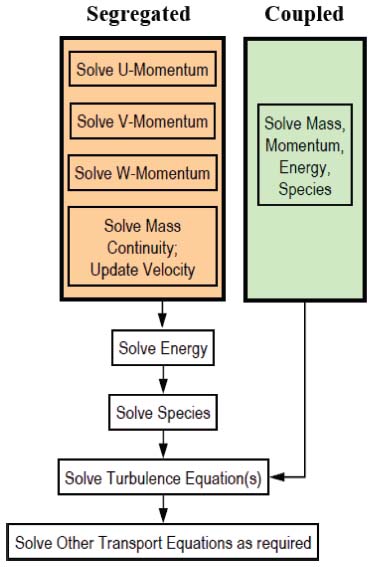
Figure 3 The procedures of the segregated and coupled methods.

The main difference between ICDB solver and the other two solvers (rhoCentralFoam and sonicFoam) is in their solution method. The solution method of ICDB solver is based on the coupled method, while the other solvers are based on the segregated method. They differ in the way that the continuity, momentum, and (where appropriate) energy and species equations are solved; the segregated solver solves these equations sequentially (i.e., segregated from one another), while the coupled solver solves them simultaneously (i.e., coupled together). The procedures of the segregated and coupled methods are shown in Figure 3.

4 Results and Discussion

The developed numerical schemes are tested for supersonic and hypersonic flows for the three cases of airflow over a flat plate, a 2-D cylinder, and a prism.

4.1 Description of Two Benchmark Test Cases

To verify and validate the ICDB solver, two test cases (flat plate and 2-D cylinder) are considered as follows:

4.1.1 Flat plate

This case is related to a hypersonic airflow over an adiabatic flat plate (Figure 4). As boundary conditions, the upper and outlet boundaries are assumed as zero gradient of pressure, velocity and temperature ($\frac{\partial p}{\partial n}\mathrm{<mo>=</mo>}0$, $\frac{\partial \overrightarrow{V}}{\partial n}\mathrm{<mo>=</mo>}0$, $\frac{\partial T}{\partial n}\mathrm{<mo>=</mo>}0$). Inlet boundary conditions for airflow are: total pressure p₀ = 648.1 Pa, total temperature T₀ = 241.5 K, and Mach number Ma = 6.47. The wall plane is adiabatic, and the fluid domain is meshed with a structured grid (Figure 5). To capture the steep gradients in the boundary layer, the mesh near the plane wall is properly fined. By a careful grid examination, it is found that a 200 × 200 grid and a distance of 20 μm (as the closest grid line to the wall of the flat plate) are appropriate.

4.1.2 2-D cylinder

This case is hypersonic airflow over an isothermal cylinder (Figure 6). The lower boundary condition is symmetric, the outlet boundary conditions are set as zero gradient ($\frac{\partial p}{\partial n}\mathrm{<mo>=</mo>}0$, $\frac{\partial \overrightarrow{V}}{\partial n}\mathrm{<mo>=</mo>}0$, $\frac{\partial T}{\partial n}\mathrm{<mo>=</mo>}0$), and inlet boundary conditions for airflow are: total pressure p₀ = 648.1 Pa, total temperature T₀ = 241.5 K, and Mach number Ma = 6.47. The wall temperature of the cylinder is 294.4 K. The fluid domain is meshed with a structured grid (Figure 7). To capture the steep gradients inside the shock wave and boundary layer, a fine mesh is used near the wall of the cylinder (The grid is 200 × 200, and the distance of the first grid line close to the wall of cylinder is 20 μm).

Figure 4 Computational domain of flat plate with boundaries.

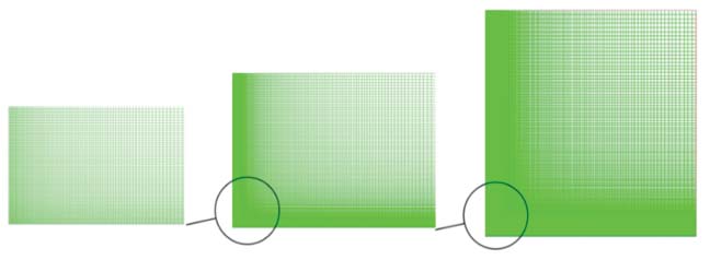
Figure 5 Structured mesh in the fluid domain for flat plate.

4.2 Case Study Description for Solver Analysis

For analysis of the solvers, the airflow over an adiabatic prism is considered. The outlet, lower and upper boundary conditions are set as zero gradient ($\frac{\partial p}{\partial n}\mathrm{<mo>=</mo>}0$, $\frac{\partial \overrightarrow{V}}{\partial n}\mathrm{<mo>=</mo>}0$, $\frac{\partial T}{\partial n}\mathrm{<mo>=</mo>}0$). Inlet boundary conditions for airflow are: total pressure p₀ = 100 kPa, total temperature T₀ = 300 K, and Mach number Ma = 1.9. The wall of the prism is adiabatic. The total computational domain and the different inlet, outlet, upper and lower boundaries of the prism are shown in Figure 8. The boundary conditions for the upper, lower and outlet faces are assumed as zero gradient, and the grid used is structured (Figure 9). A highly, but reasonably, fined mesh is adopted near the prism walls, and a mesh independent grid size of 1200 × 1200 is adopted. The distance of the first grid line close to the walls of the prism is 40 μm.

Figure 6 Computational domain of the cylinder with boundaries.

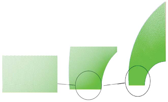
Figure 7 Structured mesh in the fluid domain for the cylinder.

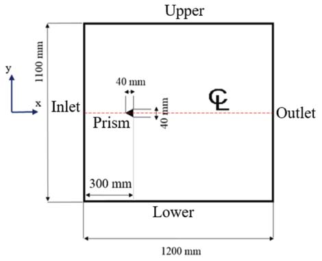
Figure 8 Computational domain of the prism with boundaries.

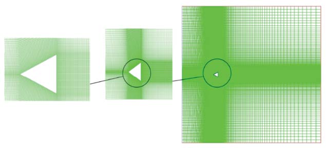
Figure 9 Structured mesh for the prism.

4.3 Verification and Validation of the ICDB Solver’s Results

First, for the flat plate, the results of ICDB solver are compared with the Chun of findings [19]. In Chun’s study, the 2nd spatial order AUSM+ and AUSM schemes have been utilized in the OpenFOAM and Fastran software, respectively.

On the other hands, the results obtained from ICDB solver are compared with the results of Chun’s study. In the present study, the 2nd spatial order AUSM⁺ up scheme is utilized in ICDB solver.

First, the contours are compared, and then the boundary aerothermal variables are compared in order to confirm the capability of ICDB solver to differentiate variables in diffusive boundary layer. The pressure and temperature contours of the present study are compared with Chun’s results in Figures 10 and 11, respectively. The predictions are in good agreement very well with each other.

The distributions of the pressures and temperatures along the flat plate are calculated by ICDB solver, and compared in Figures 12 and 13, respectively. As shown, there is no significant difference between the ICDB and Chun’s simulations.

At the flat plate’s leading edge, the results of ICDB solver and Chun’s study show oscillations. As illustrated in Figure 12, the results are quite close to each other, and the maximum difference is nearly 2%. In Figure 13, the line of ICDB is smoother than the line of solver performed by Chun. The maximum difference between the outcomes of ICDB solver and Chun’s study is approximately 3%.

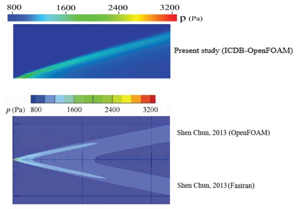
Figure 10 Comparison of the pressure contours of ICDB solver with Chun’s study [19].

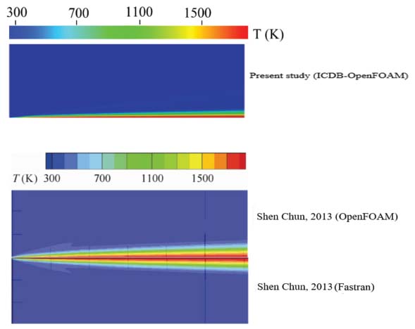
Figure 11 Comparison of the temperature contours of ICDB solver with Chun’s study [19].

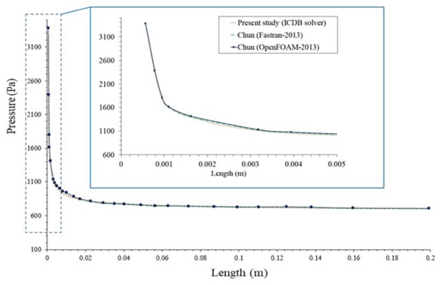
Figure 12 Comparison of the pressure distributions along the flat plate with Chun’s study [19].

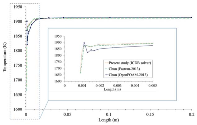
Figure 13 Comparison of the temperature distributions along the flat plate with Chun’s study [19].

It is worth mentioning that comparison of the results obtained from three schemes (AUSM, AUSM+, and AUSM⁺ up) showed their the differences well.

Here, for the cylinder case, the results of ICDB solver are compared with Chun’s results. In Chun’s study, the results have been presented by the AUSM+ solver within OpenFOAM and the 2nd order AUSM solver within Fastran. In the present study, the 2nd spatial order AUSM⁺ up scheme is utilized in ICDB solver in OpenFOAM.

Figures 14 and 15, respectively, compare the pressure and temperature contours calculated by ICDB solver with Chun’s results. The sharp gradients inside the shock wave and boundary layer can be seen clearly. As illustrated in Figure 14, for the pressure contour lines in the shock wave, the maximum contours above 35 kPa generated by ICDB is bigger than that of Fastran solver, though both of them are quite close to the results obtained by Chun using OpenFOAM. In other zones, the results are in good agreement with each other. In Figure 15, for the temperature contour lines in the shock wave, the maximum contour above 2200 K generated by ICDB is clearly bigger than that reported in Chun’s study. In other zones, the temperature contour lines from ICDB are quite close to those in Chun’s study.

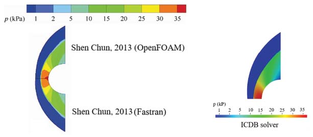
Figure 14 Comparison of the pressure contours of ICDB solver with Chun’s study [19].

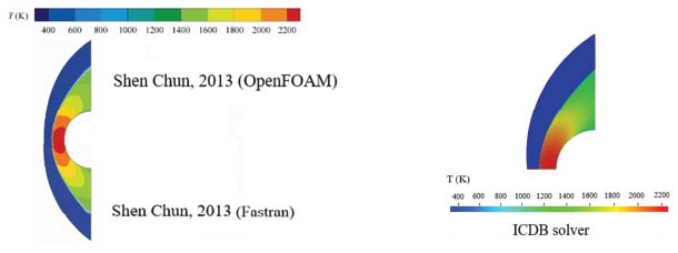
Figure 15 Comparison of the temperature contours of ICDB solver with Chun’s study [19].

Figure 16 compares the pressure distributions along the cylinder wall; as shown, the difference between the results is small. For the pressure distributions, the maximum difference between the outcome of ICDB solver and Chun’s study is nearly 5%.

The accuracy of the present study is validated by comparing with the experimental data. As shown in Figure 17, the pressure distribution of ICDB solver is in well agreement with the experimental data [19, 33]. In Figure 17, pressure is normalized with the value of inlet pressure.

Based on the above results, ICDB solver can be used as reference. Therefore, this solver is used to verify the modified sonicFoam in the next part.

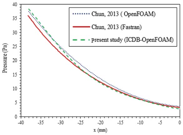
Figure 16 Comparison of the pressure distributions along the cylinder wall obtained by ICDB solver with Chun’s study [19].

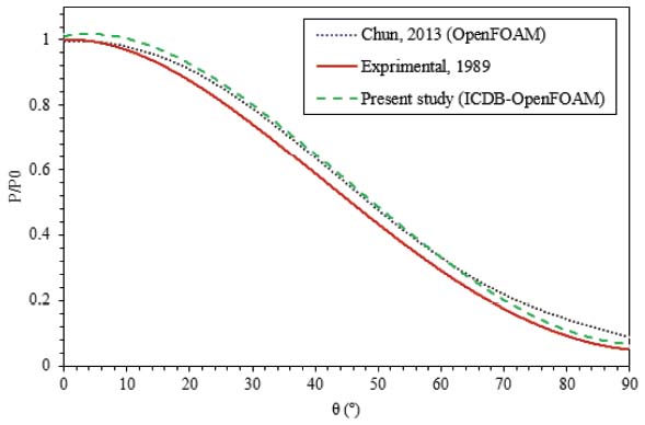
Figure 17 Comparison of the dimensionless pressure distributions along the cylinder wall obtained by ICDB solver with Chun’s study [19, 33].

4.4 Modified sonicFoam Solver’s Analysis Results

To see whether the modified sonicFoam solver has the capabilities to capture aerothermal variables or not, the airflow over an adiabatic prism as case is investigated. Due to large gradients and high turbulence levels in the prism case, the viscous dissipation rate is high. The pressure, velocity and temperature contours of sonicFoam, modified sonicFoam, rhoCentralFoam and ICDB are shown in Figure 18. As can be seen, the mechanical source ∇ · (τ · V) makes noticeable differences between the temperature fields of sonicFoam and the modified sonicFoam.

In Figure 18(a) and (b), the pressure and velocity contours produced by all the mentioned solvers are shown. Figure 18(c) illustrates that the maximum difference between the temperature contours, in comparison with ICDB solver, belongs to sonicFoam, modified sonicFoam, and rhoCentralFoam, orderly.

The pressure, velocity and temperature distributions along the central line of the prism (y = 0.0 m), the line with y = 0.01 m, and the line with y = 0.04 m are compared in Figures 19 to 21.

For better presentation, all of the obtained resulted are plotted within x = 0.2 and x = 0.5 m.

Figure 19 illustrates the pressure, velocity and temperature distributions along the center line of the prism (y = 0.0 m). There are some differences between the pressure and velocity distributions obtained by the mentioned solvers at x = 0.31–0.45 m. Also a significant difference is seen between the temperature distributions of the obtained results by sonicFoam solver with others solvers.

The temperature increases in the wake zone of the prism, where the viscous dissipation has its highest rate. It is to be mentioned that it is only in sonicFoam solver that the viscous term is neglected in the energy equation.

Figure 20 shows the pressure, velocity and temperature distributions along the line with y = 0.01 m. As clearly seen,there is no significant difference between the pressure and velocity distributions at most of the zones. For the temperature distributions, between the locations x = 0.31 m and x = 0.34 m, the difference is obvious between the sonicFoam and other solvers. The value temperature for sonicFoam is about 400 K, whereas 500 K for ICDB; this big difference is due to the effect of viscous dissipation in the wake zone of the prism. For the temperature, pressure, and velocity distributions, between the locations x = 0.34 m and x = 0.4 m, the difference between of sonicFoam and modified sonicFoam with the rhoCentralFoam and ICDB is obvious; this difference is predicted to be due to the use of different solution methods. The main differences of solution between these solvers are using the density-based and pressure-based methods. The results of rhoCentralFoam and ICDB coincide with each other. RhoCentralFoam and ICDB are density-based while sonicFoam and modified sonicFoam are pressure-based.

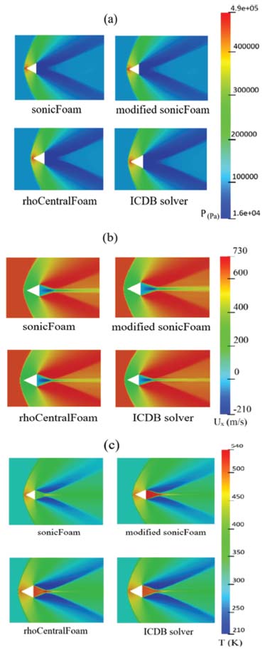
Figure 18 Pressure (a), velocity (b) and temperature (c) contours obtained from different solvers.

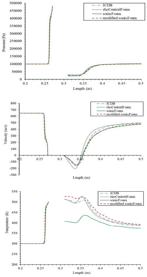
Figure 19 The distributions of characteristics of airflow along the center line of the prism (y = 0 m).

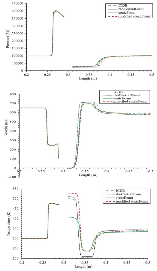
Figure 20 The distributions of characteristics of airflow along the line with y = 0.01 m.

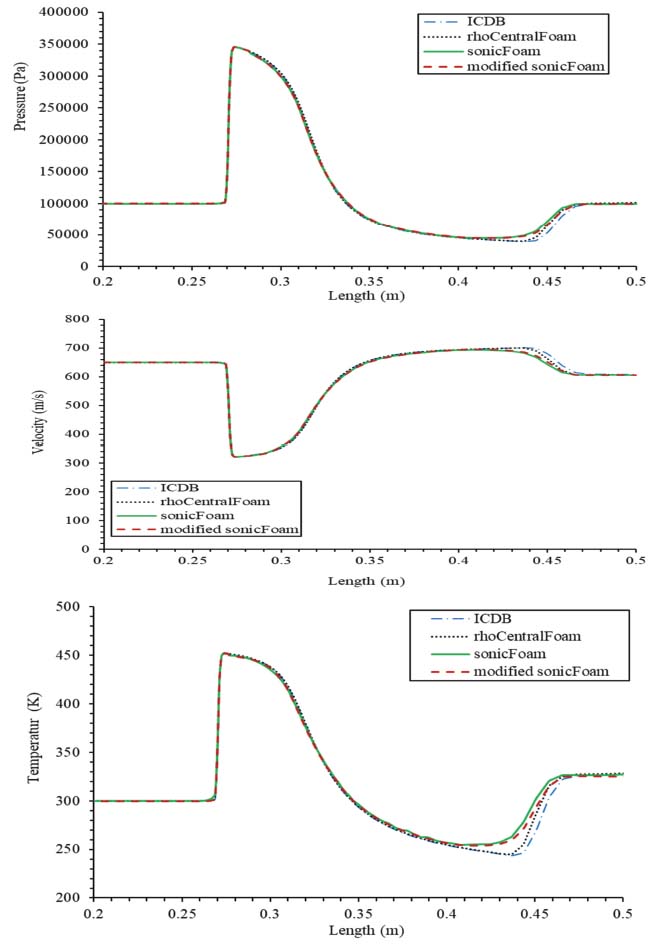
Figure 21 The distributions of characteristics of airflow along the line with y = 0.04 m.

Figure 21 illustrates the pressure, velocity and temperature distributions along the line with y = 0.04 m (y = 0.0 m is the center line of the prism). The line with y = 0.04 m is far from the prism, and the results of these plots are helpful for comparing the capability of solvers. Along the line with y = 0.04 m, the effect of viscous dissipation is less than that at y = 0.0 m and y = 0.01 m; so it would be possible to compare the effect of different solution methods in the solvers.

In Figure 21, there is no significant difference between the pressure, velocity, and temperature distributions at most of the zones. Regarding the distributions of characteristics of airflow, within x = 0.41 m and x = 0.47 m, there are some differences between the solvers. The differences are predicted to be due to difference in schemes. SonicFoam and modified sonicFoam are semi-implicit segregated pressure-based solvers with the PISO scheme, rhoCentralFoam is an explicit segregated density-based solver with the Kurganov-Tadmor’s scheme, and ICDB is an implicit coupled density-based solver with the AUSM⁺ up scheme. Based on the results presented in Section 4.3, ICDB solver is considered as reference to verify the modified sonicFoam and other solvers.

In this part, the computational efficiency of the mentioned solvers is calculated. The specification of the computational system for the prism simulation is given in Table 1.

The number of cells in the prism case is 1440000. The computational efficiency of different solvers is presented in Table 2.

Table 1 Characteristics of the computational system

CPU	Core	Speed (GHz)	RAM (GB)
INTEL	32	2.2	500

Table 2 Computational efficiency of different solvers

Solver	RhoCentralFoam	SonicFoam	Modified sonicFoam	ICDB
Time (Min)	550	380	385	230
Memory (GB)	4.8	5.2	5.2	6

It is clear from the above table that the best computational time belongs to ICDB for using the implicit coupled method. In implicit coupled method, the dependent equations are solved simultaneously. In addition, this method is more efficient; however, because of its complexity, it needs higher memory requirements. The worst computational time belongs to rhoCentralFoam for using the explicit segregated method. In explicit segregated method, the equations are independent, and can be solved separately so the memory usage is less than in other solvers. In sonicFoam and modified sonicFoam solvers, because of using the semi-implicit segregated method, the computational time is more than in full ICDB while the memory usage is less. However, since the implicit scheme is more stable than the explicit scheme, the convergence of sonicFoam and modified sonicFoam is better than that of rhoCentralFoam.

5 Conclusion

We developed an Implicit Coupled Density-Based (ICDB) solver using LU-SGS algorithm and AUSM⁺ up scheme in OpenFOAM. Also the sonicFoam solver was modified by adding the viscous dissipation term to the energy equation. To investigate the performance of the ICDB and modified sonic-Foam solvers, three typical test cases, including hypersonic airflow over a flat plate, hypersonic airflow over a cylinder and supersonic airflow over a prism were used. To validate the ICDB solver, the results were successfully compared with the experimental data and Chun’s study. To evaluate its capability in capturing the aerothermal field parameters, the modified sonicFoam solver was compared with the sonicFoam solver, and it was seen that the modified sonicFoam’s results were improved. Furthermore, the accuracy of rhoCentralFoam, sonicFoam, and modified sonicFoam as segregated solvers were compared with ICDB as coupled solver.

By investigation of the obtained results, it was concluded that ICDB enjoys the capability of modeling and simulation of supersonic and hypersonic gas flows with good computational efficiency. The most significant advantage of the solver in OpenFOAM is that a lot of other advanced methods can be directly added to it. In comparison with other analogous solvers in commercial software, it could be also further improved by other researches due to its open source characteristics.

Nomenclature

V	Velocity vector (m/s)
T	Temperature (K)
p	Pressure (Pa)
c	Speed of sound (m/s)
Ma	Mach number
D	Diagonal matrix
L	Lower-diagonal matrix
U	Upper-diagonal matrix
K	Thermal conductivity of the fluid (W/m·K)
e	Specific total energy (J/kg)
R	Universal gas constant (J·K3/mol)
M	Molar mass (kg/mol)
x,y,z	Cartesian coordinates
u,v,w	Velocity component (m/s)

Greek symbols

τ	Stress tensor
μ	Molecular coefficient of viscosity (Pa.s)
λ	Bulk coefficient of viscosity (Pa.s)
ρ	Density (kg/m3)
Φ	Viscous dissipation
∅	Vector of conservative variables

References

[1] G. Morini and M. Spiga, “The role of the viscous dissipation in heated microchannels,” ASME JJ Heat Trans, vol. 129, pp. 308–318, 2007.

[2] M. Khader, “Fourth-order predictor-corrector FDM for the effect of viscous dissipation and Joule heating on the Newtonian fluid flow,” Computers and Fluids, vol. 182, pp. 9–14, 2019.

[3] D. H. Schultz, S. Schwengels and G. Kocamustafaogullari, “Influence of viscous dissipation in a fluid between concentric rotating spheres,” Computers and Fluids, vol. 21, pp. 661–668, 1992.

[4] M. Druguet and D. Zeitoun, “Influence of numerical and viscous dissipation on shock wave reflections in supersonic steady flows,” Computers and Fluids, vol. 32, pp. 515–533, 2003.

[5] A. Zhang and B. Ni, “Three-dimensional boundary integral simulations of motion and deformation of bubbles with viscous effects,” Computers and Fluids, vol. 92, pp. 22–33, 2014.

[6] K. Stewartson, The Theory of Laminar Boundary Layers in Compressible Fluids, Oxford Univ. Press, Oxford, 1964.

[7] C. R. Nepal, T. Rahman and M. A. Hossain, “Boundary-Layer Characteristics of Compressible Flow past a Heated Cylinder with Viscous Dissipation,” Journal of Thermophysics and Heat Transfer, pp. 1533–6808, 2018.

[8] J.-M. Tanguy, Numerical Methods, USA: WILEY, 2012.

[9] K. Nerinckx, J. Vierendeels and E. Dick, “A Mach-uniform algorithm: Coupled versus segregated approach,” Journal of Computational Physics, vol. 224, pp. 314–331, 2007.

[10] K. Zhang, C. Wang and J. Tan, “Numerical study with OpenFOAM on heat conduction problems in heterogeneous media,” International Journal of Heat and Mass Transfer, vol. 124, pp. 1156–1162, 2018.

[11] OpenFOAM, “The Open Source CFD Toolbox, User Guide, ESI-OpenCFD Ltd,” 2019.

[12] P. Gaikwad and S. Sreedhara, “OpenFOAM based Conditional Moment Closure (CMC) model for solving non-premixed turbulent combustion: Integration and validation,” Computers and Fluids, vol. 190, pp. 362–373, 2019.

[13] E. Constant, J. Favier, M. Meldi, P. Meliga and E. Serrea, “An immersed boundary method in OpenFOAM : Verification and validation,” Computers and Fluids, vol. 157, pp. 55–72, 2017.

[14] M. Kraposhin, E. Smirnova, T. Elizarova and M. Istomina, “Development of a new OpenFOAM solver using regularized gas dynamic equations,” Computers and Fluids, vol. 166, pp. 163–175, 2018.

[15] A. Kurganov and E. Tadmor, “New high-resolution central schemes for nonlinear conservation laws and convection–diffusion equations,” Journal of Computational Physics, vol. 160, pp. 241–282, 2000.

[16] O. Borm, A. Jemcov and H. Kau, “Density based Navier–Stokes solver for transonic flows,” in Proceedings of the 6th OpenFOAM Workshop, USA. Penn State University, 2011.

[17] S. Chun, S. Fengxian and X. Xinlin, “Analysis on capabilities of density-based solvers within OpenFOAM to distinguish aerothermal variables in diffusion boundary layer,” Chinese Journal of Aeronautics, vol. 26, pp. 1370–1379, 2013.

[18] O. Borm, A. Jemcov and H. Kau, “Unsteady aerodynamics of a centrifugal compressor stage validation of two different CFD solvers,” in Proceedings of ASME Turbo Expo 2012, GT2012, Copenhagen, Denmark, 2012.

[19] Ansys, “http://www.ansys.com/,” 2019. [Online].

[20] Fastran, “http://www.esi-cfd.com.,” 2019. [Online].

[21] S. Chun, S. Fengxian and X. Xinlin, “Implementation of density-based solver for all speeds in the framework of OpenFOAM,” Computer Physics Communications, vol. 185, pp. 2730–2741, 2014.

[22] F. Moukalled, L. Mangani and M. Darwish, The Finite Volume Method in Computational Fluid Dynamics, Switzerland: Springer, 2016.

[23] A. Kurganov and E. Tadmor, “New high-resolution central schemes for nonlinear conservation laws and convection–diffusion equations,” Journal of Computational Physics, vol. 160, pp. 241–282, 2000.

[24] A. Kurganov, S. Noelle and G. Petrova, “Semi-discrete central-upwind schemes for hyperbolic conservation laws and Hamilton–Jacobi equations,” SIAM Journal on Scientific Computing, vol. 23, pp. 707–740, 2001.

[25] M. Kraposhin, A. Bovtrikova and S. Strijhak, “Adaptation of Kurganov-Tadmor numerical scheme for applying in combination with the PISO method in numerical simulation of flows in a wide range of mach numbers,” Procedia Computer Science, vol. 66, pp. 43–52, 2015.

[26] F. Luis, T. José and E. Sergio, “High speed flow simulaion using OpenFOAM,” in Mecánica Computacional, Salta, Argentina, 2012.

[27] M. Liou, “A sequel to AUSM, Part II: AUSM+-up for all speeds,” Journal of Computational Physics, vol. 214, pp. 137–170, 2006.

[28] P. Roe, “Approximate Riemann solvers schemes,” Computer Physic, vol. 43, pp. 357–372, 1981.

[29] K. Kitamura and A. Hashimoto, “Reduced dissipation AUSM-family fluxes: HR-SLAU2 and HR-AUSM+-up for high resolution unsteady flow simulations,” Computers & Fluids, vol. 126, pp. 41–57, 2016.

[30] S. Chun, X. linXia, Y. Wang, F. Yu and Z.-W. Jiao, “Implementation of density based implicit LU-SGS solver in the framework of OpenFOAM,” Advances in Engineering Software, vol. 91, pp. 80–88, 2016.

[31] J. Fursta, “On the implicit density based OpenFOAM solver for turbulent,” EPJ Web of Conferences, vol. 143, 2017.

[32] Y. S. M. Saad, “GMRES: A generalized minimal residual algorithm for solving nonsymmetric linear systems,” SIAM J. Sci. Statist. Comput, vol. 7, pp. 856–869, 1986.

[33] S. Ye, W. Yang and X. Xu, “The implementation of an implicit coupled density based solver based on OpenFOAM,” in Computing Machinery, Wuhan, China, 2017.

[34] B. Jiri, “Computational fluid dynamics: principles and applications,” Butterworth-Heinemann, 2015, p. 466.

Biographies

Valiyollah Ghazanfari earned a Ph.D. in nuclear engineering from Nuclear Science and Technology Institute in 2020, Iran. His research focuses on thermodynamic, fluid mechanic, CFD and numerical simulation using OpenFOAM and Fluent. He is currently working in Advanced Technology Company of Iran and Materials and Nuclear Fuel Research School.

Ali Akbar Salehi received a Ph.D. in nuclear engineering from Massachusetts Institute of Technology in 1977. He is full professor and was chancellor of Sharif University of Technology. His research focuses on Theoretical Physics. He is currently head of the Atomic Energy Organization of Iran.

Alireza Keshtkar earned a Ph.D. in chemical engineering from Tehran University, Iran. He is full professor and his research interests include design and analysis of separation processes. He is currently head of the Material and Nuclear Fuel Research School.

Mohammad Mahdi Shadman received a Ph.D. in chemical engineering from Tarbiat Modarres University, Iran. His research focuses on thermo-kinetic and fluid-mechanic in chemical engineering. He is currently working in Advanced Technology Company of Iran.

Mohammad Hossein Askari earned a Ph.D. in mechanical engineering from Tehran University, Iran. His research focuses on fluid mechanic, numerical simulation and CFD method using Fluent software. He is currently working in Advanced Technology Company of Iran.

European Journal of Computational Mechanics, Vol. 28-6, 541-572.
doi: 10.13052/ejcm2642-2085.2861
© 2020 River Publishers

Abstract

1 Introduction

2 Governing Equations

3 Numerical Schemes

3.1 rhoCentralFoam Solver

3.2 sonicFoam Solver

3.3 Modified sonicFoam Solver

3.4 ICDB (Implicit Coupled Density-Based) Solver

4 Results and Discussion

4.1 Description of Two Benchmark Test Cases

4.1.1 Flat plate

4.1.2 2-D cylinder

4.2 Case Study Description for Solver Analysis

4.3 Verification and Validation of the ICDB Solver’s Results

4.4 Modified sonicFoam Solver’s Analysis Results

5 Conclusion

Nomenclature

References

Biographies