Design and Modelling of a 90-Degree Ball Valve with a Linear Pressure Drop

Daniel A. Gutierrez¹, Jose M. Garcia-Bravo^1,*, Aaron L. Reid², Brittany A. Newell¹, Paul McPherson¹ and Mark French¹

¹School of Engineering Technology, Purdue University, West Lafayette, Indiana, USA

²Mechanical Engineer, Idex, Crawfordsville, Indiana, USA

E-mail: jmgarcia@purdue.edu

* Corresponding Author

Received 28 October 2019; Accepted 05 March 2020; Publication 30 March 2020

Abstract

Globe valves also known as ball or gate valves are used to control fluid flow in a vast number of applications. Most of the existing applications use them because of their simplicity and very low cost. However, these valves are known for their poor precision for controlling the flow and the lack of electromechanical means for their actuation. Moreover, because of their low linearity their use in closed loop control applications make them nearly unusable. The goal of this research project was to investigate means for redesigning the metering area of a ball valve in such a manner that the pressure vs. flow characteristic would be close to a linear trend. Two different profiles where designed and tested experimentally and modelled using CFD techniques for the estimation of their valve flow coefficients. The model was able to accurately predict the behaviour of the valve with less than a 10% error when fully open. The model can be used for scaling the size of the ball for larger applications and for tuning controlling strategies for flow dispensation in real life applications.

Keywords: Globe valve, flow coefficient, computational fluid dynamics.

1 Introduction

Gate and ball valves are normally used in processes requiring metered control of the volumetric flow of a fluid. A great majority of those valves are manually operated and are available in a vast number of sizes for a multitude of uses. Some of these valves have been fitted with electrical servo actuators, or rotary actuators to remotely and automatically increase or reduce the flow passing through the valve. In the specific case of ball valves, opening the valve to increase the volumetric flow results in a non-linear flow output when the valve is actuated at a constant rate. An unsteady flow output is produced when an electrically powered valve is used to produce closed loop control of the fluid, this is due to a highly unstable behaviour created by the dynamic characteristic of the flow. In automated fluid handling applications, ball valves are preferred because they can rotate from fully closed to fully opened by turning within a narrow angle (typically less than 90 degrees). Needle valves or gate valves on the other hand require multiple 360° rotations of a needle or screw to reach a fully open or closed position. Figure 1 below depicts a cross sectional view of a traditional ball valve and its principal components. The most common ball valve allows fluid to go past the ball by aligning a hole in the ball with the conduit that is attached to the valve. A stem is connected to the valve to allow the operator to rotate the ball inside the valve body. As the stem is rotated to close the valve, the hole in the valve and the conduit become mis-aligned effectively metering the flow.

A bottom-load ball valve is a type of valve where the fluid enters the valve from the bottom and exits the valve at 90 degrees through one side of the valve body. This kind of valve may have a single inlet port and two outlet ports on the sides and the electric actuator used to open and close the valve. Bottom-load valves are desirable in automated processes because they require less actuation to be completely opened/closed and can be packaged compactly and economically.

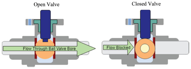
Figure 1 Ball valve cross section.

Even though, ball valves are a simple and cost effective means for controlling flow, their use in automated processes is limited due to the non-linear relationship between valve position and output flow. With an increased need for the implementation of automatic processes for IoT applications and autonomous devices, there is a need for accurate control of flow in industrial, mobile and agricultural equipment. This work focuses on the design and experimental evaluation of a ball valve capable of producing linearized flow outputs with respect to a linear control signal.

In an effort to linearize this relationship, past work and ball valve manufacturers have attempted various design geometries for the flow passage in the ball which is used as the regulating element in the valve. In a regular valve, the ball is made with a through hole perpendicular to its rotation axis (actuation). The conventional through hole has been replaced with a “V” shaped slot in an attempt to linearize the flow output with respect to the valve’s position (Kardys, 2018). This is depicted in Figure 2. In this work, this idea of linear control through adjusted geometry was modelled and experimentally tested for relationship to flow output and optimization of geometry.

In order to design and model these valves, the analysis goes back to the common orifice equation (Merritt, 1967). The valve flow coefficient, C_v, is estimated using the energy equation for an inviscid fluid in steady state, a relationship for pressure is established for flow through an orifice utilizing the well-known orifice equation (Equation (1)).

Q = C_{d} A_{o} \sqrt{\frac{2 Δ p}{ρ}}

(1)

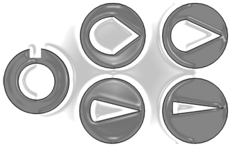
Figure 2 Standard ball (left) vs. V-Slot balls (right) (Kardys, 2018).

Where ρ is the fluid’s density and Δp is the pressure drop across the metering orifice. The terms in Equation (1) can be grouped as shown in Equation (2), then assuming ρ to be constant, a term for the valve flow coefficient is produced from lumping the contraction area, density and discharge coefficient.

Q = C_{v} \sqrt{Δ p}

(2)

The relationship presented in Equation (2) works well for establishing a relationship between flow and pressure when the area of the orifice is constant. If it was possible to keep the pressure drop Δp constant while changing the orifice area, one would clearly see that a linear increase in volumetric flow rate would produce a linear increase in the valve flow coefficient C_v. Experimental results show that this coefficient does in fact not vary linearly with flow which is ultimately determined by valve position or aperture. Because valve position is coupled to the orifice area A_o, it is therefore assumed that modifying the shape of the orifice with a specially designed geometry could produce a linear relationship between the input, valve position and the output, volumetric flow rate. This is a highly desirable characteristic of an electro-mechanical device from a systems control perspective.

The cavitation index, C_s is defined as the ratio between the pressure drop across a valve and the differential between the inlet pressure and saturated vapor pressure. The cavitation index is commonly used in industry to describe the likelihood of cavitation to occur during operation of a hydraulic component. The formulation for the cavitation index, C_s can be seen in Equation (3) below (Chern et al., 2007).

C_{s} = \frac{Δ P}{P_{i n} - P_{v}}

(3)

Where Δp is the pressure drop across the valve, p_in is the pressure at the inlet port and p_v is the saturated vapor pressure. The goal of this study is to evaluate various shapes for the orifice area using Computational Fluid Dynamics (CFD) simulation and a corresponding experimental validation of the designs.

Merritt (1967), presented an empirical characterization of the discharge coefficient with respect to the Reynolds number, in his work he discussed the influence of laminar and turbulent flow on this coefficient and noted that as the fluid behaviour approached the turbulent regime, its value asymptotically approached the constant value of 0.61. He also discussed how this was not the case for laminar flows where the discharge coefficient varied greatly between 0 and 0.68. Streeter and Wylie (1985) reported on the influence of the ratio (A_o/A₁) of the downstream area A₁ to the orifice area A_o on the discharge coefficient with respect to the Reynolds number. Their reported values of the coefficient also portray an asymptotic response for turbulent flows for various area ratios. However, the Reynolds number at which the coefficient becomes constant varies with the magnitude of the area ratio. For large area ratios (inlet to outlet area ratios larger than 70%), the discharge coefficient C_d approached a constant value at approximately Re = 40,000, which is one order of magnitude larger than the well known Reynolds number for fully turbulent flow on a pipe of circular section at approximately 2,320. On the contrary, for area ratios of 5% the C_d becomes constant at Re = 3,000. Therefore, considering the change between the upstream and downstream areas is of high importance for the study and realization of a linearized pressure to flow correlation. For the case of ball valves, the area ratio is typically large (greater than 70%), which means that the assumption of a constant discharge coefficient is reached at Re higher than 40,000. At such high turbulent flows, the effect of pipe length does not significantly diminish the turbulence behaviour of the flow.

The study conducted by Moujaes and Jagan (2008), assessed other valve coefficients that are important for characterizing the flow behaviour across ball valves. The loss coefficient, K, and the flow coefficient, C_v were used to validate the accuracy and reliability of a computational fluid dynamic model created for a ball valve. Moujaes and Jagan compared CFD data to experimental results. The flow coefficient C_v is tied to the discharge coefficient C_d as presented in Equation (1). One differs from the other in the use of the fluid’s density and geometric considerations related to the orifice area (Chern and Wang, 2004), but both represent the relationship between pressure and flow through an orifice. The study by Moujes and Jagan considered the effects of turbulence, using the continuity and momentum equations and the standard k-ε turbulence model which relates turbulence kinetic energy (k) and the rate of dissipation of turbulence energy (ε). In this study they found that the flow coefficient C_v, decreased nonlinearly with respect to the valve opening, and it also revealed that increasing the Reynolds number produced an increase in the flow coefficient mostly when the valve was opened, but trended to the same value when the valve was nearly closed. The study showed that the CFD model accurately predicted the experimental values of the flow coefficient and the models were valuable in determining the Reynolds number was not of significant importance when the valve was opened more than half.

Two partial differential equations define the turbulent kinetic energy and the rate of dissipation of turbulence energy (Hoffman and Johnson, 2007). Equation (4) describes the kinetic energy k model for turbulent flow and Equation (5) is used for the determination of energy dissipation ε.

\frac{\partial (ρ k)}{\partial t} + \frac{\partial (ρ k u_{i})}{\partial x_{i}} = \frac{\partial}{\partial x_{j}} [\frac{μ_{t}}{σ_{k}} \frac{\partial k}{\partial x_{j}}] + 2 μ_{t} E_{i j} E_{i j} - ρ ε

(4)

\frac{\partial (ρ ε)}{\partial t} + \frac{\partial (ρ ε u_{i})}{\partial x_{i}} = \frac{\partial}{\partial x_{j}} [\frac{μ_{t}}{σ_{ε}} \frac{\partial ε}{\partial x_{j}}] + C_{1 ε} \frac{ε}{k} 2 μ_{t} E_{i j} E_{i j} - C_{2 ε} ρ \frac{ε^{2}}{k}

(5)

Where:

u_i is the velocity component in the corresponding direction

E_ij is the component of rate of deformation

μ_t is the eddy viscosity

σ_k, σ_ε, C_1ε, and C_2ε are model constants

The standard k-ε model is semi-empirical, therefore the model constants are derived by several iterations of fitted data. The realizable k-ε turbulence model is very similar to the standard model, but differs in that the formulation for eddy viscosity, which describes the large-scale transport and dissipation of shear energy in a fluid. It is a variable rather than a constant (Said et al., 2016). The realizable k-ε turbulence model also differs from the standard model in that the partial differential equation that defines the rate of dissipation of turbulent energy is derived from Equations (4) and (5), for the kinetic energy term k and dissipation term ε respectively.

\begin{aligned} \frac{\partial}{\partial t} (ρ k) + \frac{\partial}{\partial x_{j}} (ρ k u_{j}) & = \frac{\partial}{\partial x_{j}} [(μ + \frac{μ_{t}}{σ_{k}}) \frac{\partial k}{\partial x_{j}}] \\ + G_{k} + G_{b} - ρ ε - Y_{M} + S_{k} \end{aligned}

(6)

\begin{aligned} \frac{\partial}{\partial t} (ρ ε) + \frac{\partial}{\partial x_{j}} (ρ k ε) & = \frac{\partial}{\partial x_{j}} [(μ + \frac{μ_{t}}{σ_{ε}}) \frac{\partial ε}{\partial x_{j}}] + ρ C_{1} S_{ε} - ρ C_{2} \frac{ε^{2}}{k + \sqrt{v ε}} \\ + C_{1 ε} \frac{ε}{k} C_{3 ε} G_{b} + S_{ε} \end{aligned}

(7)

Constant values σ_k, σ_ε, C_1ε, and C₂ are found through experimentally collected data.

The k-ω turbulence is another widely used two-term turbulence model. It is empirically based and solves for a turbulent kinetic energy term, k.

However, the k-ω model solves for the specific dissipation rate of turbulent energy, ω. The k-ω model incorporates modifications for low-Reynolds number effects that happen at the wall boundary. The k-ω model can more accurately predict the effects of wall boundary flows.

Lastly, the Reynold’s stress equation model or RSM is regarded as a more accurate turbulence model because it accounts for flows with streamline curvature, flow separation, and zones with re-circulating flows (Shih et al., 1995).

Said and his colaborators (Said et al., 2016) used the four turbulence models for obtaining the flow coefficient of a butterfly valve at different aperture angles. At an angle of 90° the valve is said to be in the fully open position. The disk angles modelled were 40°, 60°, and 70°. All the results from each CFD simulation were compared to experimental data. Of the three cases tested, the one with a 60° aperture seemed to present the best correlation between the experimental and the modelled data. A large deviation between the predicted data and the actual data was seen at 40° and some spread can be seen in the results at 70°. Overall, the models show sensitivity to disk opening and overestimate the response at low disk angles.

Procedure

This project focused on studying the influence of groove extensions on the ball orifice on the flow-position relationship. The work utilized FLUENT, a commercial CFD simulation tool for modelling fluid flow. In this study, pressure and velocity characteristics were simulated to understand the effect of complex ball valve features aimed at linearizing the response of the valve system. Experimental procedures involving 3D printed prototypes of the ball valves were used to validate the predictions made with the computational model. The steps in the process were: first, development of a CFD model to predict pressure gradient at a predetermined steady flow; second, experimental validation with a standard ball valve. The work was followed by the construction of two novel designs which were subsequently modeled using the same CFD software and experimentally validated in the same test bench. The studies presented in the review of literature have analysed the effect of manipulating the effect of simple geometry profiles on the ball, (Chern and Wang, 2004). Current literature has not focused on the effect of extended grooves on the throttling device on the valve.

The model uses the angle of aperture with respect to the closed position (measured in degrees) of the valve as the main input variable for the model and its corresponding measured flow rate. The angle of aperture is also referred to as the valve position in this document. The volumetric flow rate was preliminarily measured with respect to the angle of aperture and used as an input to the CFD model. The most important dependent variable obtained with the model was the pressure at the inlet and outlet ports of the valve. It was measured in pounds per square inch and reported here in metric units of bar.

The flow coefficient C_v was a performance measurement calculated from the resulting model using Equation (2). An experimental procedure using a flowmeter and pressure transducers was implemented to validate the pressure results obtained with the CFD model.

Volume Creation

A CAD modelling software was used to produce the geometry of the bottom load ball valve. The valve ports are 38,1 mm (1,5-inch) diameter ports at the inlet and outlet. A secondary 3D solid was made to represent the void space in the valve, this secondary solid was made for each ball design tested. For every degree of opening that a computational simulation was conducted, a unique solid was created. In total, 18 unique 3D models were created to analyse the performance of each ball grove design as seen in the representation in Figure 3.

For this CFD study, the 3D secondary solid does not represent all empty spaces that fluid occupies inside the valve. Small volumes not contributing to the generation of flow losses or pressure losses were not represented in the 3D model to simplify the meshed geometry.

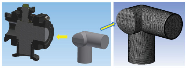
Figure 3 Secondary 3D solid model and cutaway section of the valve and corresponding meshed volume.

Model Parameters

A coarse mesh using 214,028 tetrahedral elements was made using the secondary fluid volume, and a boundary layer was used to account for the transition between turbulent and laminar flow at the wall. The growth rate used in this study was the default 0.252, meaning every element after the boundary layer has a height that was 25.2% bigger than the preceding element, the average element size was 3.2 mm. A second finer mesh using 338,572 elements of 1.6 mm average size was tested, with minimum change in the results as seen in Table 1. Perhaps the most impactful boundary condition was the velocity of the fluid at the inlet. This condition was found by converting the volumetric flow rate found from physical experimentation and solving the continuity equation Q = V ∗ A for velocity. The CFD model solved for dependent variables such as pressure drop, velocity profile, turbulent energy, etc. For all simulations an outlet pressure of 0 PSI was specified at the outlet of the ball valve. For this model it was assumed that the walls were rigid, experienced no deformation and that the fluid at the wall moves with the same velocity as the wall itself (no slip). This study assumed the flow condition to be in steady state. The fluid chosen for the model was water at a temperature of 15.5°C (60°F). The saturated water vapor pressure was assumed to be 0.018 bar (0.256 psi). The standard k-ε model was used along with the transition SST model. The transition SST model was developed by coupling the k-ω transport equations with two other transport equations. The benefit of the transition SST model is that it selects which transport equations are solved depending on the distance of an element to the wall.

Other studies using turbulence models have focused on diverse effects on geometry against flow characteristics. The study of Ye et al. (2014), characterize the effect of grooves and notches on a spool land to improve the effect of flow forces on a spool valve. Similarly, Lisowswki et al. (2017), demonstrated the usefulness of CFD turbulence models to reduce the effect of resistive forces on the spool. Likewise, Gomez et al. (2019), used CFD turbulent models to investigate the effect of the poppet and cone angle on flow characteristics at high oscillating frequencies, where it was found that reducing the angle would lead to an increased power requirement due to the development of higher flow forces.

Table 1 Comparison of turbulence models

Degree of Opening	Element Size mm [in]	Turbulence Model	Pressure Drop ΔP, Bar PSI	CFD Flow Coefficient, C_v	Exp. Flow Coefficient, C_v	Percent Diff.
90°	3.2 [0.125]	Standard k-ε	0.64 [9.23]	51.0	41.3	23.5%
90°	1.6 [0.0625]	Standard k-ε	0.69 [10.01]	49.0	41.3	18.7%
90°	1.6 [0.0625]	Transition SST	0.95 [13.83]	41.7	41.3	1.0%

At the outer layers of the boundary layer and close to the free stream area of flow, the transport equation changes to one for intermittent flow. A transport equation for the transition onset criteria determines when the transition between equations occurs (Menter et al., 2005). The standard k-ε model was used as a tool to estimate minimum element size. The results of those simulations are outlined in Table 1. The flow coefficient predicted by the standard k-ε model was approximately 18.7% higher than the experimental flow coefficient as described in the experimental section below. For the same given mesh, a computational simulation using the transition SST model was conducted. The computational flow coefficient using the transition SST model was only 0.99% higher than the experimental flow coefficient. These flow coefficients and percent differences compare the standard ball design at its fully open position.

Experimental Measurements

Experiments were carried out to validate the accuracy of the CFD model. Three ball designs were manufactured and tested to collect experimental data that was later compared to CFD modelled data. Each ball design features a 38.1 mm (1.5-inch) diameter inlet and outlet. Of the three designs, the standard ball is manufactured from 316 stainless steel and has the finest surface finish. The other two ball designs, design 1 and design 2, were fabricated using additive manufacturing and are made of ABS plastic. Design 1 and design 2 had a rougher surface finish than the standard ball. Images of the tested balls are shown in Figure 4.

The standard ball differs from the other two designs in that it rotates from its fully closed to fully open position in a 90° turn. Both design 1 and design 2 ball prototypes take approximately 180° to travel from fully closed to the fully open position. This is because design 1 and design 2 balls feature an outside groove that gradually increases as the orifice is rotated from its fully closed to fully open positions.

Figure 4 CAM models of standard design (left), design 1 (centre) and design 2 (right).

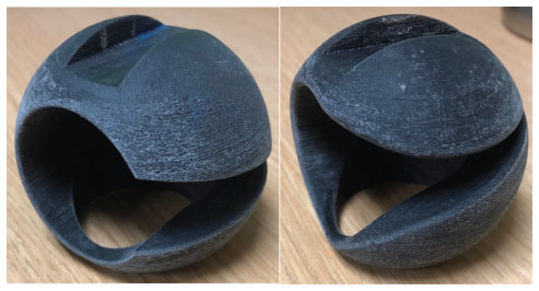
Figure 5 Actual 3D printed balls used for design 1 and design 2 valves.

Equipment Used

To capture the experimental data, several measurement devices and tools were used. Figure 6 shows a schematic representation of the simple test circuit used to test each ball design and the location of each measurement device in the circuit.

Each measurement device and component is labelled in Figure 7, the flowmeter and open tank are not shown in the picture. The direction of flow is shown with the arrow markers. A magnetic flow meter was used to measure the flow after the test valve. The line downstream of the bottom-load ball valve returns fluid to an open tank.

An indicator to measure the aperture angle for each ball design was 3D printed to fit over the ball valve housing. The indicator had a resolution of 5° and a range of 0°–180°. An image of this indicator can be seen below in Figure 8.

Testing Procedure

For the experimental procedure the prime mover attached to the pump was run continuously for approximately 60 seconds or until a steady flow output was seen on the digital screen of the flowmeter. The stabilized flow measurement was recorded in units of U.S. gallons per minute (GPM). Once the system reached a steady state condition, the pressure values were recorded using the pressure transducers and data acquisition system. Measurements of steady state pressure and flow were recorded for each aperture angle, the aperture angle was modified during the test in increments of 15 degrees. Each aperture position was also used for the simulation study. The same procedure was carried out for each of the experimental balls shown in Figure 4. Considering that the viscosity of water varies minimally with respect to temperature changes (0.024 cSt per °C) (Trostmann, 2000), it is expected that minimum error will be incurred by moderate temperate or pressure increases. All measurements were conducted at room temperature (22°C) and near sea level atmospheric pressure (∼1 atm).

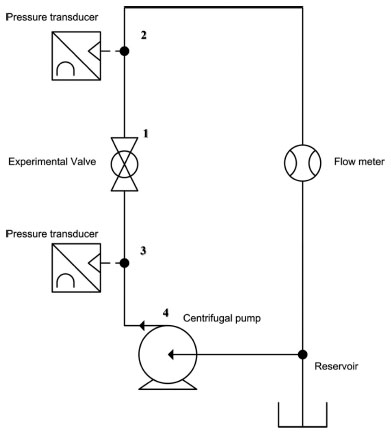
Figure 6 Test circuit schematic.

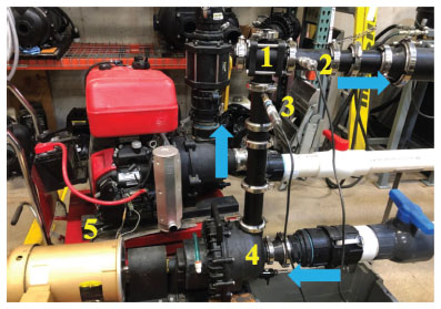
Figure 7 Actual test circuit.

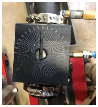
Figure 8 Angle indicator.

Results

Experimental Results

Standard ball design

As expected, the experimental results show a non-linear relationship between flow coefficient and valve aperture. The data collected from the testing procedure is listed in Table 2 below. The experimental valve flow coefficient C_v was estimated from the flow and differential pressure measurements and Equation (2).

Computational Modelling Results

Table 3 below lists the estimated values from the CFD simulation at 6 different aperture values of the standard ball valve, the rightmost column shows the estimated percent difference between the experimental value and the calculated value from the model for the flow coefficient. Figure 9 demonstrates a comparison of the pressure drop across the experimental and the computational model of the standard valve.

Table 2 Experimental test data (standard ball)

Aperture [°]	Pressure In Bar [PSI]	Pressure Out Bar [PSI]	Pressure Drop Bar [PSI]	Flow-Rate lpm [GPM]	Flow Coefficient, C_v
90°	0.7 [10]	−0.3 [−4.1]	1.0 [14.1]	586 [155]	41.28
75°	0.7 [10.2]	−0.3 [−4.4]	1.0 [14.6]	563 [149]	39.00
60°	1.1 [15.5]	−0.3 [−4.8]	1.4 [20.3]	525 [139]	30.85
45°	1.9 [27.6]	−0.5 [−6.6]	2.4 [34.2]	412 [109]	18.64
30°	2.8 [40.2]	−0.5 [−7.6]	3.3 [47.8]	201 [53.1]	7.68
15°	3.1 [44.9]	−0.2 [−3.2]	3.3 [48.1]	76 [20.2]	2.91

Table 3 Computational analysis of a standard ball

Aperture [°]	Pressure In Bar [PSI]	Flow-rate lpm [GPM]	Computational Flow Coefficient, C_v	Experimental Flow Coefficient, C_v	Percent Differen
90°	1.0 [13.8]	586 [155]	41.69	41.28	1.0%
75°	1.0 [13.8]	564 [149]	40.04	39.00	2.7%
60°	1.1 [16.6]	526 [139]	34.08	30.85	10.5%
45°	1.9 [27.7]	413 [109]	20.71	18.64	11.1%
30°	4.6 [67.0]	201 [53.1]	6.49	7.68	15.5%
15°	3.1 [44.9]	76 [20.2]	3.01	2.91	3.4%

The percent difference values between the experimental and CFD data for the flow coefficient is shown in Table 3 and plotted in Figure 10. From this data it can be seen that the computational simulation tends to predict the flow coefficient most accurately in flows that exhibit relatively less turbulence near full aperture or full closure of the valve. As the aperture decreases, the turbulence created becomes more complex and difficult to model. To accurately capture an increasingly complex turbulence, a progressively finer mesh would be required. The experiments carried out by Chern and Wang (2004) and the simulations by Moujaes and Jagan (2008) demonstrate that closing of the valve at low aperture angles generate vortexes that reduce the effective passage of the flow, therefore choking the flow and giving rise to exaggerated pressure at the inlet as it was observed at 30 degrees of aperture in Figure 9 in the experimental results and the CFD simulation.

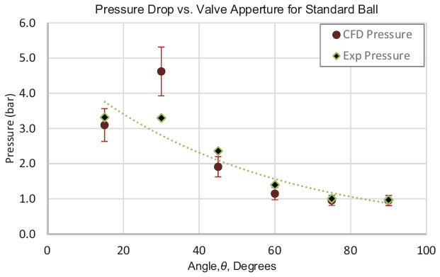
Figure 9 Flow characteristics.

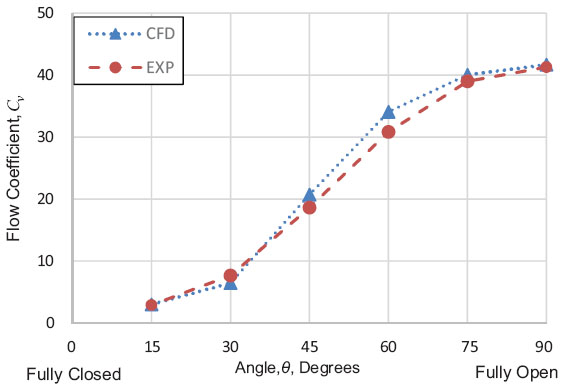
Figure 10 Comparison of flow coefficient curves (standard ball).

Experimental Measurements of New Designs

Design 1 ball

The experimental results for Design 1 do not exhibit a linear relationship between flow coefficient and aperture. The data collected from the testing procedure can be seen in Table 4 above. Similarly, the valve coefficient was estimated using equation 2. Because the groove on Design 1 was elongated, the aperture increments were made in steps of 30° instead of 15° as was done for the standard ball.

Table 4 Experimental test data (design 1)

Aperture [°]	Pressure In Bar [PSI]	Pressure Out Bar [PSI]	Pressure Drop Bar [PSI]	Flow-rate lpm [GPM]	Experimental Flow Coefficient, C_v
180°	0.3 [4.85]	−0.3 [−4.9]	0.7 [9.75]	612 [162]	51.88
150°	0.4 [6.01]	−0.3 [−4.71]	0.7 [10.72]	597 [158]	48.26
120°	1.7 [24.14]	−0.4 [−5.28]	2.0 [29.42]	559 [148]	27.29
90°	2.0 [28.45]	−0.4 [−5.2]	2.3 [33.65]	393 [104]	17.93
60°	2.5 [36.5]	−0.5 [−7.5]	3.0 [44]	291 [77]	11.61
30°	2.7 [39.8]	−0.4 [−6.1]	3.2 [45.9]	193 [51]	7.53

Table 5 Experimental test data (design 2)

Aperture [°]	Pressure In Bar [PSI]	Pressure Out Bar [PSI]	Pressure Drop Bar [PSI]	Flow-rate lpm [GPM]	Experimental Flow Coefficient, C_v
180°	0.4 [5.55]	−0.3 [−4.74]	0.7 [10.29]	612 [162]	50.50
150°	0.6 [8.64]	−0.3 [−4.94]	0.9 [13.58]	582 [154]	41.79
120°	1.2 [17.56]	−0.3 [−4.9]	1.5 [22.46]	514 [136]	28.70
90°	2.1 [30.43]	−0.5 [−7.6]	2.6 [38.03]	374 [99]	16.05
60°	2.7 [38.75]	−0.4 [−5.6]	3.1 [44.35]	234 [62]	9.31
30°	3.0 [43.8]	−0.1 [−1.5]	3.1 [45.3]	102 [27]	4.01

Design 2 ball

The experimental results for the second ball design exhibit a more linear relationship between flow coefficient and aperture than Design 1 and the standard ball. Table 5 above lists the measured flow rate and pressure drops obtained for various aperture levels.

A comparison of the experimental results for each of the tested ball designs can be seen in Figure 11. A linear regression analysis was run to measure the linearity of each experimental ball tested, the R² coefficient was used to compare which ball design was a better fit to a straight line. Even though the behaviour of the valves was not perfectly linear, the aim is to use the prototype profiles to follow this type of response as closely as possible. Where the standard valve results could be fitted to a line with an R² value of 0.97, the Design 1 valve and R² value of 0.94, and the Design 2 valve an R² value of 0.98. Based on the obtained correlation coefficient values, the experimental data collected in this study demonstrated that the ball using the Design 2 groove presented a response that was closest to a line between flow and flow coefficient versus the aperture.

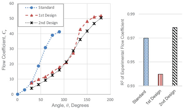
Figure 11 Comparison of experimental flow coefficient curves.

Similarly, Figure 12 below shows the trend for the flow output versus the aperture angle, the linear fit shown in this figure was pictured without including the last data point from the experiment, in the case of the Design 1 valve the R² correlation value was found to be 0.98 and for Design 2 it was 0.99.

Computational Modelling Results for Proposed Designs

The results of all 6 computational simulations for design 1 and design 2 can be seen in Table 6 below. Because the grove on the ball is elongated, the full aperture of the ball is achieved at 180° with the proposed designs. The corresponding flow coefficient was estimated for each degree of opening matching to the measured flow rate measured and reported in for the experimental test described in the preceding experimental section.

The data is plotted in Figure 13, depicts the experimental and simulated flow coefficients for various aperture angles. At low apertures, the coefficients seem to be very close to each other for Design 1 and Design 2 in both the experimental and the CFD simulation datasets. However, as the aperture is increased beyond 120 degrees, it was observed that the flow coefficient increased at a rate higher than that exhibited by a linear trend. Interestingly, when opening values near the maximum value, the trend decreased for the experimental methods, but kept increasing in both the CFD simulations for Design 1 and 2. This discrepancy can be attributed to the presence of entrained air in the system.

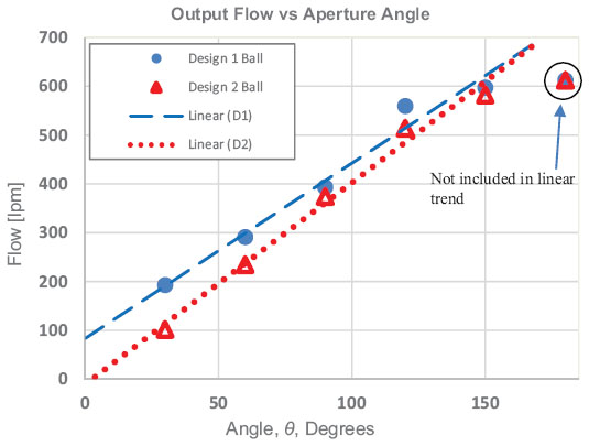
Figure 12 Comparison of experimental flow coefficient curves.

Table 6 Computational analysis of design 1 and design 2 valve

Degree of Opening	Design 1 Pressure Drop, ΔP, Bar [PSI]	Design 2 Pressure Drop, ΔP, Bar [PSI]	Design 1 Computational Flow Coefficient, C_v	Design 2 Computational Flow Coefficient, C_v
180°	0.6 [9.3]	0.5 [6.6]	63.01	53.07
150°	0.6 [9.2]	0.5 [7.5]	56.31	52.20
120°	1.4 [20.7]	0.9 [12.6]	38.39	32.50
90°	1.5 [22.4]	1.4 [20.8]	21.75	21.97
15°	1.8 [26.6]	2.6 [38.4]	10.01	14.93
30°	3.4 [49.1]	5.5 [80.5]	3.01	7.28

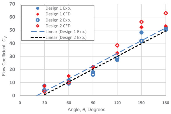
Figure 13 Comparison of flow coefficient curves for design 1 and design 2.

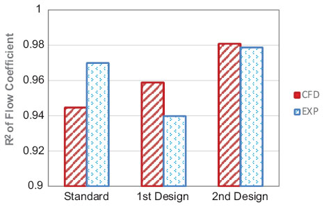
Figure 14 R² comparison of computational and experimental methods.

The R² values for flow coefficient were found to differ significantly between valve prototypes as is shown in Figure 14. This is because the computational models calculate pressure drop across the fluid domain based on a variety of parameters including, mesh quality and size, turbulence model, boundary conditions, fluid properties, etc.

Both the computational and experimental method show that Design 2 most closely fits a linear regression line with a 95% confidence level. However, the computational model does not agree with experimental data for Design 1. The Design 1 ball had the highest percent difference between computational and experimental results of the three designs analysed in this study.

Discussion and Conclusions

The CFD model’s accuracy to predict flow was validated using experimental data for a standard ball valve and two 3-D printed custom made ball valve bodies with wide grooves. Each of the three ball designs were manufactured and tested in this circuit. The standard ball design is a production part and was readily available in 316 stainless steel with a fine surface finish. Design 1 and Design 2 ball designs were created through additive manufacturing and made of ABS plastic. Because the maximum pressure at valve is less than 10 bar, and the tensile strength of ABS is approximately 455 bar, the risk of deformation and leakage is minimum.

A comparison of data from the computational and experimental methods (Figure 11) show that the CFD model can predict flow coefficient with very good accuracy up to 83.3% of the full valve aperture value. One of the primary factors that influence the accuracy of a CFD model is the turbulence model chosen to simulate turbulence created by the fluid domain. It is expected that at higher aperture levels, the level of turbulence and flow is higher, making the system harder to model. The possibility of cavitation forming at low degrees of opening is another factor that could affect the CFD model. In this study a single phase CFD model was used for all computational analyses. To accurately model the effects of cavitation, a multi-phase CFD model must be used.

The computational and experimental methods agree that modifying the design of a traditional bottom-load ball to the second ball design would increase the linearity of its flow coefficient curve with respect to degree of opening.

In conclusion, the CFD model was observed to generally predict the relationship between flow coefficient and degree of opening for a ball design. Values for flow coefficient were most accurately predicted for the standard ball and the Design 1 ball at the fully open positions and to all designs in the nearly closed positions. The average percent difference between computational and experimental methods was 9.35% at the fully open position.

Percent difference between methods was observed to grow in the intermediate aperture positions. This may be due to a variety of factors including representation of the fluid domain, mesh quality, turbulence model, and cavitation.

Lastly, this study found that the modifications found in the second ball design (Design 2) increase linearly the flow coefficient, the linearity for this design was estimated to be the best as measured by the R² coefficient, but it also saw the greatest percentage error between the CFD model and experimental data at the fully opened positions.

References

Chern, M. J. and Wang, C. C. (2004). Control of volumetric flow-rate of ball valve using V-port. Transactions-American Society of Mechanical Engineers Journal of Fluids Engineering, 126, 471–481.

Chern, M.-J., Wang, C.-C., and Ma, C.-H. (2007). “Performance test and flow visualization of ball valve.” Experimental thermal and fluid science 31(6): 505–512.

Gomez, I., Gonzalez-Mancera, A., Newell, B., and Garcia-Bravo, J. (2019). Analysis of the Design of a Poppet Valve by Transitory Simulation. Energies, 12(5), p. 889.

Hoffman, J. and Johnson, C. (2007). Computational turbulent incompressible flow: Applied mathematics: Body and soul 4 (Vol. 4). Springer Science & Business Media.

Kardys, G. (2018). “Characterized and V-Ball Valves Provide Improved Flow Control”, Engineering 360, IEEE GlobalSpec, Nov. 1, 2018 Accessed online December 15, 2018 from: https://insights.globalspec.com/article/10415/characterized-and-v-ball-valves-provide-improved-flow-control

Lisowski, E., Filo, G., and Rajda, J. (2018). Analysis of Flow forces in the initial phase of throttle gap opening in a proportional control valve, Flow Measurement and Instrumentation, Volume 59, 2018, Pages 157–167, ISSN 0955-5986, doi.org/10.1016/j.flowmeasinst.2017.12.011.

Menter, F. R., Langtry, R., Völker, S., and Huang, P. G. (2005). Transition Modelling for General Purpose CFD Codes. In Engineering Turbulence Modelling and Experiments 6. https://doi.org/10.1016/B978-008044544-1/50003-0

Merritt, H. E. (1967). Hydraulic control systems. John Wiley & Sons.

Moujaes, S. F., and Jagan, R. (2008). 3D CFD Predictions and Experimental Comparisons of Pressure Drop in a Ball Valve at Different Partial Openings in Turbulent Flow. Journal of Energy Engineering, 134(1), 24–28. https://doi.org/10.1061/(ASCE)0733-9402(2008)134:1(24)

Said, M. M., AbdelMeguid, H. S., and Rabie, L. H. (2016). The Accuracy Degree of CFD Turbulence Models for Butterfly Valve Flow Coefficient Prediction. American Journal of Industrial Engineering, 4(1), 14–20.

Shih, T. H., Zhu, J., and Lumley, J. L. (1995). A new reynolds stress algebraic equation model. Computer Methods in Applied Mechanics and Engineering, 125(1–4), 287–302.

Streeter, V. L. and Wylie, E. B. (1985). Fluid Mechanics. 8th Ed, McGraw Hill.

Trostmann, E. (2000). Tap Water as a Hydraulic Pressure Medium. CRC Press.

Ye, Y., Yin, C., Li, X., Zhou, W., and Yuan, F. (2014). “Effects of groove shape of notch on the flow characteristics of spool valve,” Energy Conversion and Management, Volume 86, Pages 1091–1101, ISSN 0196-8904, doi.org/10.1016/j.enconman.2014.06.081.

Biographies

images

Daniel A. Gutierrez received a B.S. in Mechanical Engineering Technology and an M.S. in Engineering Technology from Purdue University West Lafayette in 2017 and 2019. In 2019 he began working as a research and design engineer for Banjo Corporation, a fluid handling device manufacturer in the agricultural industry. As an engineer at Banjo Corporation he has used various Computer-Aided Engineering technologies to design and improve products. His research interests include multi-physics modeling for real-world applications, primarily fluid-structure interactions.

images

Jose M. Garcia-Bravo received a B.S. in Mechanical Engineering from Universidad de Los Andes in 2002Bogota, Colombia, and M.Sc. in Engineering and Ph.D. degrees from Purdue University West Lafayette, IN, USA. in 2006 and 2011 respectively. From 2011 to 2012, he was a Research Assistant Professor at the Illinois Institute of Technology. Since 2015, he has been an Assistant Professor with the School of Engineering Technology at Purdue University, West Lafayette. His research interests include electric and hydraulic hybrid drive trains, Additive manufacturing of hydraulic and pneumatic components and energy efficiency and duty cycles of hydraulic systems.

images

Aaron L. Reid received a B.S. in Mechanical Engineering from Rose-Hulman Institute of Technology, Terre Haute, IN, USA in 1994. From 1994 to 1996, Aaron worked as a Project Engineer at Cadillac Rubber and Plastics, Cadillac, MI. In 1996, Aaron went to work for Banjo Corporation, Crawfordsville, IN, an agricultural liquid handling products company, as a Project engineer. Throughout his time at Banjo Corporation, Aaron has performed cradle to grave product design and development, plastic injection molding and machining department manager for 10 years, and currently design engineering manager leading the product engineering team.

images

Brittany A. Newell received a B.S. degree in Biomedical Engineering, a M.Sc. and Ph.D. in Agricultural and Biological Engineering from Purdue University West Lafayette, IN, in 2009, 2010, and 2012 respectively. From 2013 to 2015, she worked for a contract manufacturing company in quality and regulatory engineering and as a Quality Manager. In 2015, she returned to Purdue as an Assistant Professor with the school of Engineering Technology. Her research interests are intelligent sensors and actuators, adaptive structures, additive manufacturing, and energy efficiency. Dr. Newell is interested in implementation of these technologies into industrial applications.

images

Paul McPherson is an Assistant Professor of Practice in the School of Engineering Technology at Purdue University, Paul teaches both mechanical design and quality control courses. Professor McPherson’s research interests include quality systems in manufacturing for process improvement, mechanical design and analysis, and education about technical standards.

images

Mark French Received a B.S. in Aerospace and Ocean Engineering from Virginia Tech in 1985. He received an M.S. in 1988 and Ph.D. in 1993, both in Aerospace engineering from the University of Dayton. He worked as a civilian engineer for the US Air Force from 1985 to 1995, specializing in aeroelasticity and photomechanics. He then moved to the automotive industry, where he was a lab manager for Lear Corp from 1995–1999. He moved to Bosch, where he was a senior engineer in their Noise and Vibration group from 1999–2004. He then came to Purdue, where his now a professor in the School of Engineering Technology. He works primarily on industrial engagement, experimental mechanics and stringed instrument design.