Optimisation of a Pump-Controlled Hydraulic System using Digital Displacement Pumps

L. Viktor Larsson^1,*, Robert Lejonberg${}^2$ and Liselott Ericson${}^1$

¹Division of Fluid and Mechatronic Systems (Flumes), Department of Management and Engineering (IEI), Linköping University, Linköping, Sweden
²Epiroc Rock Drills AB, Örebro, Sweden
E-mail: mailto:viktor.larsson@liu.seviktor.larsson@liu.se; mailto:robert.lejonberg@epiroc.comrobert.lejonberg@epiroc.com; mailto:liselott.ericson@liu.seliselott.ericson@liu.se
^*Corresponding Author

Received 31 August 2021; Accepted 30 September 2021; Publication 12 November 2021

Abstract

When electrifying working machines, energy-efficient operation is key to maximise the use of the limited capacity of on-board batteries. Previous research indicate high energy savings by means of component and system design. In contrast, this paper focuses on how to maximise energy efficiency by means of both design and control optimisation. Simulation-based optimisation and dynamic programming are used to find the optimal electric motor speed trajectory and component sizes for a scooptram machine equipped with pump control, enabled by digital displacement pumps with dynamic flow sharing. The results show that a hardware configuration and control strategy that enable low pump speed minimise drag losses from parasitic components, partly facilitated by the relatively high and operation point-independent efficiencies of the pumps and electric motor. 5–10% cycle energy reductions are indicated, where the higher figure was obtained for simultaneous design and control optimisation. For other, more hydraulic-intense applications, such as excavators, greater reductions could be expected.

Keywords: Control optimisation, simulation-based optimisation, pump control, digital displacement pump, mobile hydraulics.

Extended Publication

This paper is an extended version of [1]. The extension is the outer plant optimisation loop with associated theory, results, discussion and conclusion.

1 Introduction

Mining machines are mobile working machines used to move ore and other granular material in mines. Currently, these machines are subject to electrification, with decreased global use of energy and fossil fuels as primary motivators. For mining machines, a lowered energy consumption is directly related to cost for the user, but electrification also has positive side effects. By replacing the conventionally used combustion engine with an electric power source, local emissions such as exhaust gases, heat and noise are reduced. This reduction, or even elimination, improves the working environment for the machine operator and reduces the need for ventilation, which is a major energy consumer in a mine.

For electrified solutions with on-board batteries, limited energy capacity compared to diesel fuel puts high requirements on the energy efficiency of the machine’s motion system. This aspect is challenging in particular for the work functions, that conventionally are powered by a hydraulic system with throttle control. In pump-controlled hydraulic systems, valve throttling is minimised by powering each function with an individual pump [2].

Traditionally, pump-controlled systems have been difficult to motivate as they require the pumps to be dimensioned for the maximum flow of each function. With several functions, this results in an expensive system with multiple large pumps that primarily operate at part load with poor efficiency [3]. In this paper, the use of a digital displacement pump (DDP) is considered as a measure to mitigate the above-mentioned drawbacks of pump control.

1.1 Scope and Delimitations

The aim of this paper is to, in terms of energy efficiency, evaluate the potential of the concept presented in Section 2 applied to the Epiroc ST14 Battery, and to investigate the gains of optimising the concept with respect to both component sizing and control of the electric motor shaft speed. The work functions considered are boom, bucket and steering while the driveline is not within the scope of the paper. The current available DDP version from Danfoss is considered, which operates in pump-mode only [4]. Energy recuperation from the loads is thus not considered.

1.2 Scooptram

The mining machine considered in this paper is referred to as scooptram. Similar to a wheel loader, a scooptram uses articulated steering and has a loader with boom and bucket. In contrast to the wheel loader a scooptram is, however, designed to be used under ground, and therefore has stricter space requirements, which results in a rather compact design. The specific machine model studied in this paper is the Epiroc ST14 Battery [5], shown in Figure 1. It has a battery (Li-Ion NMC) as primary energy source, which is swapped to a recharged battery when empty. This concept allows battery charging from the grid and machine operation to occur simultaneously. The ST14 Battery uses one electric motor (traction motor) for propulsion and another (auxiliary motor) to power the work functions (boom, bucket and steering). Today, the work functions are implemented with a conventional load sensing system with two axial-piston pumps connected in parallel. This paper explores the potential of replacing each axial-piston pump with a Danfoss Digital Displacement Pump (DDP) [4], shown in Figure 2.

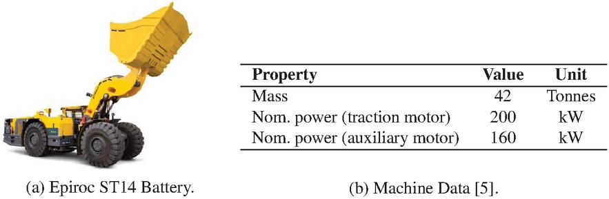
Figure 1 Scooptram application considered in the paper.

1.3 Digital Displacement Pump

A DDP is a piston pump where the flow is controlled by individually connecting and disconnecting each piston to the pump’s high and low pressure sides, enabled by actively controlled high-speed solenoid valves [6]. The pump displacement is then varied by controlling the number of active and non-active pump cylinders during one or several shaft revolutions [4]. Within the scope of this paper, it is assumed that this property is equivalent to the continuously variable displacement in a conventional pump.

A benefit with the DDP design is that it yields higher part load efficiencies compared to conventional axial piston pumps. This benefit was showcased in the 16-tonnes DEXTER excavator, where a swap from axial piston pumps to DDPs resulted in fuel savings of up to 20% with maintained productivity [7].

Another attractive feature of the DDP is that its physical layout facilitates access to the individual pistons. One pump can thus be treated as several pumps connected in parallel on the same shaft. Each pump, referred to as pumplet, can in turn be dedicated to an individual function [8]. If each pumplet flow is individually controlled, a system solution classified as a centralised pump-controlled system with mechanical power distribution [2] can thereby be achieved. In this paper, in contrast to [8], the DDPs are powered by an electric motor with variable speed, which presents a degree of freedom.

From a control perspective, a pump with variable speed and variable displacement has a degree of freedom since the pump flow is the product of these two variables. Traditionally, this freedom has been locked by considering either constant speed or constant displacement, primarily due to cost reasons [2]. One recent exception is [9], where a speed-controlled pump with discretely variable displacement is considered. As previously mentioned, this paper assumes continuously variable pumplet displacements.

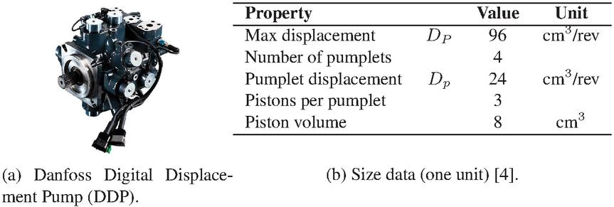
Figure 2 Danfoss Digital Displacement Pump (DDP).

1.4 Dynamic Programming

To lock the degree of freedom, optimal control is considered in this paper, using deterministic Dynamic Programming (DP). With DP, the control problem is discretised in state-time, where a recorded drive cycle is used to find the optimal control decision for each discrete time instant of the cycle, proceeding backward in time. The primary benefit with DP is that it yields the globally optimal solution (for a given discretisation). This benefit does, however, come with two important drawbacks. The first is a high computational cost, that increases exponentially with the number of states and control signals considered. The other is that it requires knowledge of the complete cycle, which means that the obtained control strategy is not implementable in practice. Rather, the results from the DP optimisation can be used to develop and evaluate causal control strategies. This is common practice within research of hybrid vehicles, where a DP result is commonly used as benchmark when evaluating energy management strategies, see for instance [10]. In this paper, the use of DP serves primarily two purposes:

• To explore the maximum potential of the considered system concept.

• To provide knowledge on how to optimally control the concept.

1.5 Combined Plant and Control Optimisation

While control optimisation locks time-dependent control degrees of freedom, plant optimisation deals with time-independent design parameters, such as component sizes. For a given system, the control and plant optimisation problems are usually coupled, in the sense that the optimal design depends on the employed control strategy and vice versa. Depending on how strong this coupling is, different strategies for combined plant and control optimisation may be applied. In this paper, the bi-level strategy according to the classification in [11, 12] is used, in which an outer loop finds the optimal design, and an inner loop finds the optimal control strategy for each design candidate. The primary reason for this choice is that the bi-level strategy can guarantee global optimality, which is required when exploring a system’s maximum potential.

2 System Concept

Figure 3 shows the concept investigated in the paper. The conventional pumps in the ST14 Battery are replaced with DDPs ($P_1$ and $P_2$) connected to two valve blocks, while the rest of the system is unchanged. The three loads are controlled with directional valves ($V_1$–$V_3$) that are assumed fully open when the load cylinders are in motoring mode and are used for meter-out throttling when the load cylinders are in pumping mode. The boom and bucket functions have bypass valves that are assumed to be controlled simultaneously with the directional valve of each function, to redirect some of the flow from the piston side chamber to the piston rod side chamber when the cylinder is in pumping mode, thereby reducing the required pump flow.

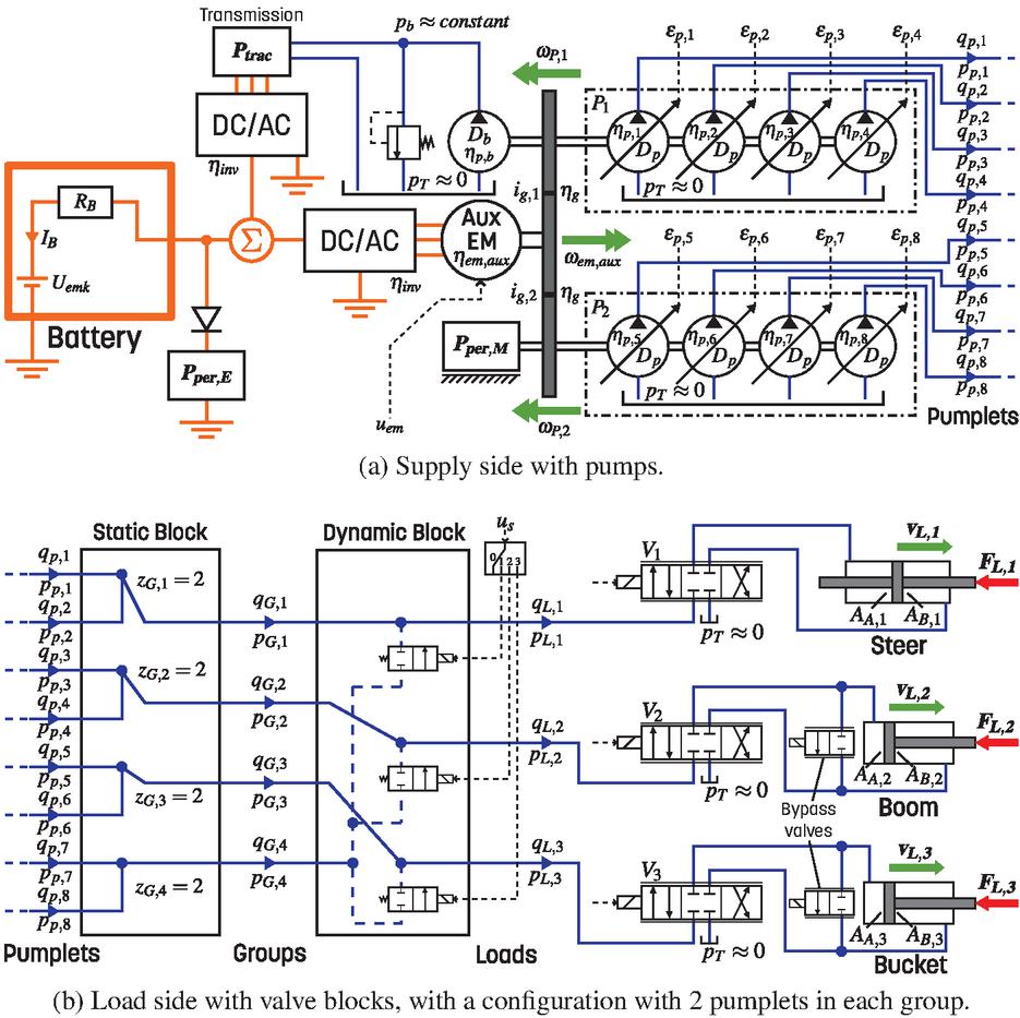
Figure 3 Layout of the system to be optimised. States that are determined directly by the drive cycle in the optimisation are highlighted in bold. Any check valves for load holding purposes are omitted in the figure.

The pumplets are connected to a static block which combines the pumplets into groups. Figure 3 shows a configuration with two pumplets in each group. The static block configuration may, however, be regarded as an open question, and is handled by the plant optimisation in this paper. The dynamic block connects the pumplet groups to the loads. In contrast to the static block, the dynamic block can change during use of the system, thereby enabling dynamic flow or pumplet allocation [8]. The idea of the concept is to dedicate group 1, 2 and 3 to load 1, 2 and 3, respectively, and have group 4 available as a shared resource. For instance, if 100 l/min is required by load 1, but group 1 can only provide 50 l/min, group 4 can provide the remaining 50 l/min. This enables moderate pumplet sizes as the loads seldom require their maximum flow simultaneously for the considered application.

The DDPs are powered by the auxiliary electric motor (Aux EM) which also powers peripheral mechanical functions ($P_{per,M}$, e.g. brakes, cooling) and the transmission clutch boost circuit, which consists of a fixed displacement gear pump ($D_b$) connected to a pressure relief valve. The auxiliary and traction ($P_{trac}$) electric motors are powered by the battery which also powers peripheral electric functions ($P_{per,E}$, e.g. A/C, battery cooling).

As previously discussed, the speed of the auxiliary electric motor is a free variable, and there is a compromise to make between shaft speed and flow sharing. This compromise is found using control optimisation in this paper.

3 Problem Formulation

To explore the considered concept’s maximum potential, it is optimised with combined plant and control optimisation. In the applied bi-level strategy, the plant is optimised by an outer loop that generates design candidates. Each candidate, in turn, is evaluated by an inner control optimisation loop. In this paper, the inner loop uses DP, which ensures each inner evaluation is optimal.

3.1 Dynamic Programming

The control optimisation problem is formulated as:
u_em(t)E_B(u_em(t),
¯
Λ
(t),X)
0 ≤ε_p,k(t)≤1, k = 1,2,…, z_p
u_s(t)= j, j ∈[0,1,…, z_L]
u_em,min ≤u_em(t)≤u_em,max
I_B,min(t) ≤I_B(t)≤I_B,max(t)
ω_em,aux,min(t)≤ω_em,aux(t)≤ω_em,aux,max
˙
ω
_em,aux(t)=u_em(t)
ω_em,aux(t_0)=ω_em,aux,min(t_0)
ω_em,aux,min(t_f)≤ω_em,aux(t_f)≤ω_em,aux,max
where $u_{em}(t)$ is the control signal, which is the angular acceleration of the auxiliary electric motor. This choice of control signal is made to enable limitation in shaft acceleration and thus avoid solutions with undesired and unrealistic shattering of the motor speed. It may also be noted that the introduction of the angular acceleration defines the angular speed as a state, which makes the optimal solution time-dependant. From a strict mathematical perspective, $u_{em}(t)$ may also be interpreted as an additional degree of freedom. $\overline{\mathrm{\Lambda }}(t)$ is the drive cycle:

$$\overline{\mathrm{\Lambda }}(t)=\left[\begin{array}{c}\hfill F_{L,i}(t)\hfill \\ \hfill v_{L,i}(t)\hfill \\ \hfill \mathrm{⋮}\hfill \\ \hfill F_{L,z_L}(t)\hfill \\ \hfill v_{L,z_L}(t)\hfill \\ \hfill P_{trac}(t)\hfill \\ \hfill {\omega }_{em,aux,min}(t)\hfill \end{array}\right],\text{with}t\in [t_0,t_f]$$

(1)

where $F_{L,i}(t)$ and $v_{L,i}(t)$ is the force and velocity of load $i$, respectively. $P_{em,trac}(t)$ is the power to the driveline and ${\omega }_{em,aux,min}(t)$ is the minimum speed of the auxiliary motor as required from the driveline transmission to obtain sufficient flow to its boost circuit. $t_0$ and $t_f$ are the starting time and final time of the drive cycle, respectively. The cost to minimise is the total energy consumed by the battery during the cycle:

$$E_B={\int }_{t_0}^{t_f}-P_{B,ch}(t)dt$$

(2)

where $P_{B,ch}(t)$ is the battery charging power ($P_{B,ch}>0$ for charging, $P_{B,ch}\le 0$ for discharging). $X$ is the design parameter vector, which is chosen by the outer (plant) optimisation loop and thus regarded as given for the control optimisation problem.

3.2 Plant Optimisation

The design parameters of the outer loop are the pump gear ratios and the number of pumplets in each group. By assuming that a group cannot be empty and that all available pumplets, $z_p$, are used, it is sufficient to include all groups except for the last one in the design parameter vector:

$$X=[i_{g,1},i_{g,2},z_{G,1},\mathrm{\dots },z_{G,z_G-1}]$$

(3)

where $i_{g,l}$ is the gear ratio of pump $l$, $z_{G,j}\in [1,2,\mathrm{\dots }]$ is the number of pumplets in group $j$ and $z_G$ is the total number of groups. The number of pumplets in the last group is calculated according to:

$$z_{G,z_G}=z_p-\sum _{j=1}^{z_G-1}{z}_{G,j}$$

(4)

Since $z_{G,z_G}\ge 1$, the outer loop optimisation problem may then be formulated as:
XE_B(X)
∑_j=1^z_G-1 z_G,j≤z_p-1
1 ≤z_G,j ≤z_p-(z_G-1), j = 1,2,…, z_G
i_g,l,min ≤i_g,l≤i_g,l,max,l = 1,2
where the first constraint is included as a penalty function in the objective function in the implementation.

4 Model

The DP algorithm uses a backward-facing simulation model to evaluate the cost-to-go at each time step. The input to this model is thus the drive cycle, $\overline{\mathrm{\Lambda }}(t)$, the design variables, $X$, and the grid of states and control signals. In the following equations, this means that ${\omega }_{em,aux}$ is regarded as given.

Some important modelling assumptions:

1. Constant tank pressure, $p_T\approx 0$.

2. Each control valve ($V_{1,2,3}$) and on/off valve in the dynamic valve block yield a constant pressure drop $\mathrm{\Delta }{p}_v=5$ bar.

3. Lossless cylinders.

4. When active, the bypass valves are controlled so that the full piston rod chamber flow is supplied by the piston chamber flow.

5. The pumplets’ displacements are continuously variable.

6. Lossless static valve block.

4.1 Cylinders

The steering motion of the scooptram is actuated with two identical asymmetric cylinders connected in parallel. This arrangement is modelled as an equivalent symmetric cylinder. Similarly, the boom function’s two cylinders are modelled as an equivalent asymmetric cylinder. Assumptions 1–3 yield the load pressure $p_{L,i}$ for load $i$:

$$p_{L,i}=\{\begin{array}{cc}\frac{F_{L,i}+\mathrm{\Delta }{p}_v{A}_{A,i}}{A_{B,i}}+\mathrm{\Delta }{p}_v\hfill & P_{L,i}>0,v_{L,i}>0\hfill \\ \frac{\mathrm{\Delta }{p}_v{A}_{A,i}-F_{L,i}}{A_{B,i}}+\mathrm{\Delta }{p}_v\hfill & P_{L,i}>0,v_{L,i}\le 0\hfill \\ \mathrm{\Delta }{p}_v\hfill & P_{L,i}\le 0\hfill \end{array}$$

(5)

where $P_{L,i}$ is the power consumed by load $i$:

$$P_{L,i}=F_{L,i}{v}_{L,i}$$

(6)

The load flow $q_{L,i}$ for load $i$ is:

$$q_{L,i}=\{\begin{array}{cc}{v}_{L,i}{A}_{A,i}\hfill & v_{L,i}>0\hfill \\ -v_{L,i}{A}_{B,i}\hfill & v_{L,i}\le 0\hfill \end{array}$$

(7)

For the boom and bucket functions, assumption 4 yields:

$$q_{L,i}=0\mathit{\hspace{1em}}\text{for}{P}_{L,i}\le 0,v_{L,i}\le 0,i\in [2,3]$$

(8)

4.2 Dynamic Valve Block

The configuration of the dynamic valve block is a function of the control signal $u_s$, which is implicitly defined by ${\omega }_{em,aux}$ after the introduction of the following rules:

1. Flow sharing is only used when a group is saturated,

2. When flow is shared, the load flow is divided between the saturated and shared pumplet groups in proportion to the maximum available flow of these groups,

3. The flow of each pumplet group is divided between the pumplets connected to this group in proportion to the maximum available flow of these pumplets,

To decide if sharing should occur, the maximum flow available at each group can first be calculated as:

$${\overline{q}}_{G,max}=\left[\begin{array}{c}\hfill q_{G,max,1}\hfill \\ \hfill \mathrm{⋮}\hfill \\ \hfill q_{G,max,z_G}\hfill \end{array}\right]={\overline{M}}_{PG,q}{\overline{q}}_{p,max}={\overline{M}}_{PG,q}\left[\begin{array}{c}\hfill q_{p,max,1}\hfill \\ \hfill \mathrm{⋮}\hfill \\ \hfill q_{p,max,z_p}\hfill \end{array}\right]$$

(9)

where $z_G$ is the total number of groups and $z_p$ is the total number of pumplets. ${\overline{M}}_{PG,q}={\overline{M}}_{GP,p}^T$ is a $[z_G\times z_p]$ matrix with zeros and ones that correspond to the connections in the static valve block (see further details in Section 4.3). For the considered concept:

$$q_{p,max,k}=\{\begin{array}{cc}{D}_p{\omega }_{P,1}\hfill & 1\le k\le 4\hfill \\ D_p{\omega }_{P,2}\hfill & 5\le k\le z_p\hfill \end{array}$$

(10)

where ${\omega }_{P,l}$ is the shaft speed of pump $l$:

$${\omega }_{P,l}=i_{g,l}{\omega }_{em,aux}$$

(11)

where $i_{g,l}$ is the gear ratio of the gear connecting pump $l$ to the auxiliary electric motor. Define $j_{sat}$ as the group index at which group flow is saturated:

$$q_{L,j_{sat}}>q_{G,max,j_{sat}},j_{sat}\in [1,2,\mathrm{\dots },z_L]$$

(12)

where $z_L$ is the total number of loads. According to rule 2 the flow, $q_{G,j}$, at group $j$ is then determined as:

$$q_{G,j}=\{\begin{array}{cc}{q}_{L,i}\hfill & i\ne j_{sat}\hfill \\ q_{L,i}\frac{q_{G,max,i}}{q_{G,max,i}+q_{G,max,zG}}\hfill & i=j_{sat}\hfill \end{array},j\in [1,2,\mathrm{\dots },z_L]$$

(13)

The flow at the shared group is:

$$q_{G,z_G}=\{\begin{array}{cc}0\hfill & i\ne j_{sat}\hfill \\ q_{L,i}-q_{G,i}\hfill & i=j_{sat}\hfill \end{array}$$

(14)

and finally the group pressures are:

$$p_{G,j}=\{\begin{array}{cc}{p}_{L,j}\hfill & j\in [1,2,3]\hfill \\ \{\begin{array}{cc}0\hfill & i\ne j_{sat}\hfill \\ p_{L,i}+\mathrm{\Delta }{p}_v\hfill & i=j_{sat}\hfill \end{array}\hfill & j=4\hfill \end{array}$$

(15)

4.3 Static Valve Block

To determine the pumplet flows and pressures, the group flows and pressures are first collected in the vectors ${\overline{q}}_G$ and ${\overline{p}}_G$, respectively:

$${\overline{q}}_G=\left[\begin{array}{c}\hfill q_{G,1}\hfill \\ \hfill \mathrm{⋮}\hfill \\ \hfill q_{G,z_G}\hfill \end{array}\right],{\overline{p}}_G=\left[\begin{array}{c}\hfill p_{G,1}\hfill \\ \hfill \mathrm{⋮}\hfill \\ \hfill p_{G,z_G}\hfill \end{array}\right]$$

(16)

Similarly, the pumplet flows and pressures are collected as:

$${\overline{q}}_p=\left[\begin{array}{c}\hfill q_{p,1}\hfill \\ \hfill \mathrm{⋮}\hfill \\ \hfill q_{p,z_p}\hfill \end{array}\right],{\overline{p}}_p=\left[\begin{array}{c}\hfill p_{p,1}\hfill \\ \hfill \mathrm{⋮}\hfill \\ \hfill p_{p,z_p}\hfill \end{array}\right]$$

(17)

Ignoring pressure losses in the static valve bock, the pumplet pressures can then be determined by:

$${\overline{p}}_p={\overline{M}}_{GP,p}\cdot {\overline{p}}_G$$

(18)

where ${\overline{M}}_{GP,p}$ is a $[z_p\times z_G]$ matrix with ones and zeros that corresponds to the connections in the static valve block. Note that ${\overline{M}}_{GP,p}$ depends on the configuration set by the outer optimisation loop (via $z_{G,j}$). For example, for the configuration shown in Figure 3 ($z_{G,j}=2$ for all $j$):

$${\overline{M}}_{GP,p}=\left[\begin{array}{cccc}\hfill 1\hfill & \hfill 0\hfill & \hfill 0\hfill & \hfill 0\hfill \\ \hfill 1\hfill & \hfill 0\hfill & \hfill 0\hfill & \hfill 0\hfill \\ \hfill 0\hfill & \hfill 1\hfill & \hfill 0\hfill & \hfill 0\hfill \\ \hfill 0\hfill & \hfill 1\hfill & \hfill 0\hfill & \hfill 0\hfill \\ \hfill 0\hfill & \hfill 0\hfill & \hfill 1\hfill & \hfill 0\hfill \\ \hfill 0\hfill & \hfill 0\hfill & \hfill 1\hfill & \hfill 0\hfill \\ \hfill 0\hfill & \hfill 0\hfill & \hfill 0\hfill & \hfill 1\hfill \\ \hfill 0\hfill & \hfill 0\hfill & \hfill 0\hfill & \hfill 1\hfill \end{array}\right]$$

(19)

Ignoring leakage and obeying rule 3, the pumplet flows are:

$${\overline{q}}_p={\overline{M}}_{GP,q}\cdot {\overline{q}}_G$$

(20)

where ${\overline{M}}_{GP,q}$ is a $[z_p\times z_G]$ matrix with each element:

$${\overline{M}}_{GP,q}(k,j)=\frac{q_{p,max,k}}{q_{G,max,j}}$$

(21)

4.4 Pumps

The relative displacement, ${\epsilon }_{p,k}$, of pumplet $k$ connected to pump $l$ can then be determined according to:

$${\epsilon }_{p,k}=\frac{q_{p,k}}{D_p{\omega }_{P,l}}$$

(22)

The total efficiency, ${\eta }_{p,k}$, of pumplet $k$ connected to pump $l$ is then calculated with linear interpolation in an efficiency map obtained from the pump manufacturer:

$${\eta }_{p,k}=f({\omega }_{P,l},p_{p,k},{\epsilon }_{p,k})$$

(23)

The efficiencies are used to calculate the input power to each pumplet:

$$P_{p,k}=\frac{q_{p,k}{p}_{p,k}}{{\eta }_{p,k}}$$

(24)

which yield the pump torques according to:

$$T_{P,1}=\frac{{\sum }_{k=1}^4{P}_{p,k}}{{\omega }_{P,1}},T_{P,2}=\frac{{\sum }_{k=5}^{z_p}{P}_{p,k}}{{\omega }_{P,2}}$$

(25)

4.5 Mechanical Losses

The boost circuit for the driveline transmission is modelled as a constant torque, assuming ideal pressure relief valve characteristics:

$$T_{b,trac}=\frac{p_b{D}_b}{{\eta }_{p,b}}$$

(26)

where $p_b$ is the boost pressure, $D_b$ the boost pump volumetric displacement and ${\eta }_{p,b}$ the boost pump hydromechanical efficiency (assumed constant, ${\eta }_{p,b}\approx 0.8$). Other peripheral mechanical losses are modelled as a constant power loss, estimated from the drive cycles:

$$T_{per,M}=\frac{P_{per,M}}{{\omega }_{P,2}}$$

(27)

4.6 Auxiliary Electric Motor

The total torque on the auxiliary electric motor is then:

$$T_{em,aux}=\frac{T_{P,1}+T_{b,trac}}{{\eta }_g}{i}_{g,1}+\frac{T_{P,2}+T_{per,M}}{{\eta }_g}{i}_{g,2}$$

(28)

where ${\eta }_g$ are the gear efficiencies (assumed constant, ${\eta }_g\approx 0.98$). The efficiency, ${\eta }_{em,aux}$, of the auxiliary electric motor is calculated with linear interpolation in an efficiency map obtained from the motor manufacturer:

$${\eta }_{em,aux}=f(T_{em,aux},{\omega }_{em,aux})$$

(29)

which yields the input power to the auxiliary electric motor:

$$P_{em,aux,in}=\frac{T_{em,aux}{\omega }_{em,aux}}{{\eta }_{em,aux}}$$

(30)

4.7 Electric Circuit

The battery output power is calculated as:

$$P_B=-P_{em,trac}-\frac{P_{em,aux,in}}{{\eta }_{inv}}-P_{per,E}$$

(31)

where $P_{per,E}$ is electric peripheral losses, which are assumed constant and were estimated from the drive cycle. ${\eta }_{inv}$ is the inverter efficiency (assumed constant). $P_{em,trac}$ is the power to the driveline electric motor:

$$P_{em,trac}=\{\begin{array}{cc}\frac{P_{trac}}{{\eta }_{inv}}\hfill & P_{trac}\ge 0\hfill \\ P_{trac}{\eta }_{inv}\hfill & P_{trac}<0\hfill \end{array}$$

(32)

where $P_{trac}$ is the power to the driveline recorded during the drive cycle. The battery current, $I_B$, is then obtained as:

$$I_B=\frac{-U_{emk}}{2R_B}+\sqrt{{\left(\frac{U_{emk}}{2R_B}\right)}^2+\frac{P_B}{R_B}}$$

(33)

where $U_{emk}$ and $R_B$ are the electromotive force voltage and the internal resistance of the battery, respectively, both assumed to be constant and which values were obtained from the battery manufacturer. This finally yields the battery charge power:

$$P_{B,ch}=P_B-R_B{I}_B^2$$

(34)

5 Drive Cycle

A short loading cycle (two repetitions, $t_f=140$ seconds, $t_0=0$) that was recorded with a ST14 Battery operated by a professional operator was used for the optimisation. In the recorded cycle, the machine fills the bucket in a gravel pile, reverses, turns, drives to another pile and empties the bucket.

After recorded, the results were post-processed to obtain some of the states used in the optimisation (see Equation (1)). The piston forces were calculated from the logged cylinder pressures and the cylinder dimensions, assuming lossless cylinders. The boom piston position was first calculated from the logged boom angle and geometrical data and then differentiated and filtered with a moving average filter to obtain the piston velocity. Similarly, the steer piston velocity was obtained from the steer angle while the bucket velocity was calculated from the logged piston position. The driveline power was calculated from the logged torque and speed of the driveline electric motor. The recorded minimum required speed of the auxiliary motor was scaled with the pump 1 gear ratio ($i_{g,1}$), as the boost pump for the transmission clutch circuit is connected to the same shaft as pump 1 (see Figure 3).

6 Results and Discussion

The optimisation problem was solved in Matlab with the Complex RF algorithm [13] as outer loop and DP as inner loop using the implementation in [14] with the settings in Table 3 (appendix). Time discretisation was made with a step size of 0.2 seconds, which is regarded as the minimum actuation time of the dynamic block valves. To minimise risk of local optimum, the outer optimisation was run 100 times, from which the best solution was selected. 3 optimisations stopped due to limit in maximum number of evaluations (2500) and the rest stopped due to convergence in objective function value.

The resulting state trajectory (auxiliary motor shaft speed), the shared group load dedication ($u_s(t)$) and the pumplet group pressures for the optimised cycle are shown in Figure 4 while the group and load flows are shown in Figure 5. The control optimisation maximises the shared group use to minimise the auxiliary motor speed. Parts of the cycle require higher shaft speed to match the required flow, which can be observed in Figures 4–5 as the bucket filling phases (20–40 seconds and 80–100 seconds) and the boom raising phases (50–70 seconds and 110–120 seconds). It may also be noted that the outer loop has chosen group sizes and gear ratios that minimise flow outputs from the pumplets of pump 1, which minimises its required speed.

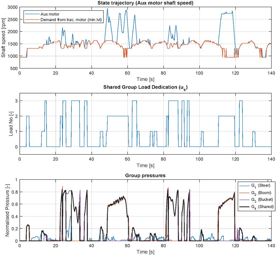
Figure 4 Auxiliary motor speed, flow sharing control signal and normalised group pressures for the optimised (plant$+$control) cycle.

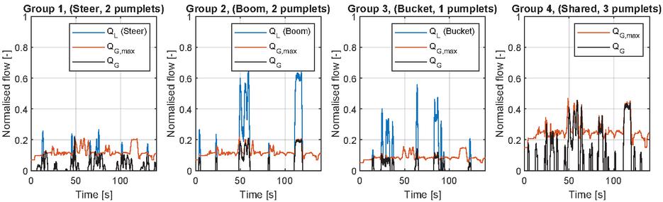
Figure 5 Optimal pumplet group configurations and normalised group and load flows for the optimised (plant$+$control) cycle.

To investigate the gains of optimising the system with respect to control and/or design, three additional cases were considered. These are summarised in Table 1 along with the previously described case (Plant$+$ctrl opt.).

In Table 1, default configurations denote cases where no outer (plant) optimisation loop was used. For these configurations, one with constant shaft speed and another with optimised shaft speed was studied, with default values of the static block configurations and gear ratios. The constant speed case was carried out as a DP optimisation with constant speed, chosen as the lowest value possible to manage the cycle.

The optimised configurations in Table 1 denote cases where an outer optimisation loop has been used. The plant + control optimisation case is the case shown previously in Figures 4–5. The plant optimisation case is the constant speed case optimised with the same outer loop as described in Section 3, with the addition that the shaft speed was included as a design variable. 100 optimisations were also run for this case, where 34 optimisations failed to converge within the maximum number of function evaluations (2500), and the rest stopped due to convergence in objective function value.

Table 1 Default${}^1$ and (plant) optimised${}^2$ configurations

Case ($\downarrow$), Parameter ($\to$)	$z_{G,1}$	$z_{G,2}$	$z_{G,3}$	$z_{G,4}$	$i_{g,1}$	$i_{g,2}$	${\omega }_{em,aux}$
Const. speed${}^1$	2	2	2	2	1	1	2800 rpm
Ctrl opt.${}^1$	2	2	2	2	1	1	variable
Plant opt.${}^2$	2	2	1	3	0.61	0.84	2963 rpm
Plant $+$ ctrl opt.${}^2$	2	2	1	3	0.61	0.89	variable

Figure 6 shows bubble plots for the pumps and the auxiliary electric motor for the different cases. In these figures as well, it is clear that low speed of pump 1 is preferred, since all optimised cases result in minimised speed of this unit. It was found that the major reason for this was the power loss due to the transmission boost circuit pump, which is connected to the same shaft as pump 1 (see Figure 3). This loss increases proportionally to the pump speed and is significantly larger (approximately a factor 2) than the losses in the pumps and the electric motor. For the control optimisation case (yellow), pump and electric motor efficiencies are compromised due to their relatively low importance compared to the boost circuit loss. When adding the outer loop as well (lilac), enough freedom is given for also improving the electric motor and pump efficiencies. These results highlight the benefits of considering the complete system rather than the individual components when evaluating energy efficiency, and of having high and relatively flat (operation point-independent) efficiencies in the pumps and electric motors. For the ST14 Battery machine, the results also suggest that an alternative solution for the boost circuit could be interesting.

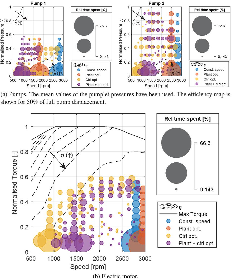
Figure 6 Bubble plots for the pumps and the auxiliary electric motor.

The cycle energies for the different cases are shown in Figure 7, where the baseline case (load-sensing with axial-piston pumps) is also shown for comparison. Compared with the baseline case, the total cycle energy was decreased with 5% using constant speed. The primary cause for the improvements were found to be reduced pump losses and reduced valve throttling losses. Plant optimisation, control optimisation and combined plant and control optimisation added an additional drop of 3, 4 and 5%, respectively, primarily caused by reduced losses in the transmission boost circuit pump. One source of error are the peripheral electrical losses ($P_{per,E}$), which were difficult to estimate and stands for approximately 7–8% of the total cycle total energy. This indicates a need to investigate these losses in more detail.

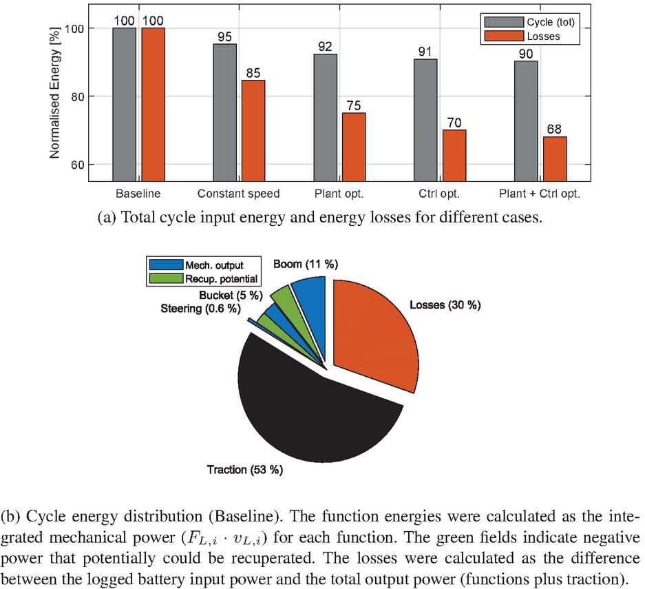
Figure 7 Cycle energy. The baseline cycle energy was calculated from the recorded battery current and voltage.

Compared to [7, 8], the obtained improvements may be considered surprisingly small. In [7, 8], the application is, however, an excavator with a diesel engine, where parts of the savings were achieved by selecting a more fuel-optimal point of the engine. In addition, all power is actuated with the hydraulic system in an excavator while the driveline represented 53 % of the energy consumption for the scooptram in the considered cycle (see Figure 7b). Moreover, in contrast to an excavator, simultaneous use of multiple hydraulic functions is rare in a scooptram, which results in low pressure-compensating losses in the baseline case. The gains from introducing pump control in the considered application are therefore relatively low compared to the excavator considered in [8].

Compared to the constant speed case, the results indicate that approximately 4% extra energy savings are gained by optimally controlling the electric motor speed, where the gains are almost exclusively due to the lowered losses in the transmission boost circuit. This improvement is in the same order of magnitude as was found for the truck loader crane in [9], and may be seen as moderate. One important reason for this improvement being moderate is that the pumps and the electric motor both have relatively high efficiency for a large operational domain, which therefore makes the speed parameter of less importance (efficiency-wise) for these components. This aspect is emphasised further when studying the effect of optimising the plant and control together, which yielded merely 2 extra percent in energy saving compared to plant optimisation and 1 extra percent compared to control optimisation. The relatively low improvement when optimising both plant and control also indicates that the coupling between them is rather weak in this application.

Although they may seem moderate, the improvements due to control and/or plant optimisation are still desirable due to the fact that scooptrams often operate non-stop in short loading cycles. It should be noted though, that hardware changes, such as the gear ratios, may have significant influence on other aspects than the energy consumption, and therefore be more difficult to implement in practice compared to a new control strategy. On this same topic, all the presented results are based on one drive cycle, and other cycles may lead to different solutions.

Furthermore, it may be noted that the boom and bucket functions have high amounts of energy that could potentially be recuperated, which would further lower the energy losses.

Concerning the outer (plant) optimisation problem (3.2) it may be noted that the number of pumplets in each group ($z_{G,j}$) are integers, while Complex RF uses real numbers. In the implementation, this was handled by rounding the numbers provided by Complex RF. The risk with this approach is that the optimisation converges prematurely since the rounding function implies that all real numbers close to the integer yield the same objective function value (plateaus). The use of the randomisation factor and the high number of optimisation runs should, however, minimise this risk [13].

7 Conclusions and Outlook

The Digital Displacement Pump facilitates the implementation of pump control in a mobile working machine. Using combined plant and control optimisation, the maximum potential of the considered pump control concept with dynamic flow sharing could be evaluated. The results show that a hardware configuration and control strategy that minimises pump speed is preferred, primarily due to drag losses in the transmission clutch actuation boost circuit. The strategy is facilitated by the high and relatively operation point-independent efficiencies of the pumps and electric motor. The results indicate a 5% decrease in total system energy use for the considered short loading cycle, with an additional 4 % drop if the electric motor speed is optimally controlled and an additional 1% drop if the static group allocation and pump gear ratios are optimised as well. The improvements mainly come from reduced valve throttling, pump losses and transmission boost circuit losses.

The low amount of simultaneous function use in the considered application suggest that greater loss reductions is to be expected for a more hydraulic-intense application, such as an excavator. Moreover, the obtained results depend on the considered concept and the load cycle. It should also be emphasised that the obtained optimal strategy is not directly implementable in a causal controller, which indicate lower savings in a final application. Other applications, load cycles, concepts and development of causal control strategies are, consequently, subjects for future work.

Acknowledgements

This research was funded by the Swedish Energy Agency (Energimyndigheten, Grant Number 50181-2), Volvo Construction Equipment AB and Epiroc AB. The authors would particularly like to thank Simon Magnusson and Markus Bagge at Eiproc for their input concerning the ST14 Battery machine, and Kim Heybroek at Volvo Construction Equipment for valuable input on working machines.

Nomenclature

Designation	Denotation		Unit
$A_{A/B}$	A/B-side piston area		m${}^2$
$D$	Volumetric displacement		m${}^3$/rad
$\mathrm{\Delta }{p}_v$	Valve pressure drop		Pa
$E$	Energy		J
$\epsilon$	Relative displacement		–
$\eta$	Efficiency		–
$F$	Force		N
$I$	Current		A
$i_g$	Gear ratio		–
$\overline{\mathrm{\Lambda }}$	Drive cycle		(vector)
${\overline{M}}_{GP,p/q}$	Static valve block pressure/flow matrix (Groups $\to$ pumplets)		(matrix)
${\overline{M}}_{GP,p/q}$	Static valve block pressure/flow matrix (Groups $\to$ pumplets)		(matrix)
$E$	Energy		J
$\omega$	Rotational speed		rad/s
$P$	Power		W
$p$	Pressure		Pa
$q$	Flow		m${}^3$/s
$R$	Resistance		Ohm
$T$	Torque		Nm
$t_0$	Cycle start time		seconds
$t_f$	Cycle end time		seconds
$U$	Voltage		V
$u_{em/s}$	Electric motor/ flow sharing control signal		rad/s${}^2$ (–)
$v$	Velocity		m/s
$X$	Design parameter vector		(vector)
$z_G$	Total number of groups ($z_G$ = 4 here)		–
$z_{G,j}$	Number of pumplets in group $j$		–
$z_L$	Total number of loads ($z_L$ = 3 here)		–
$z_p$	Total number of pumplets ($z_p$ = 8 here)		–
Subscripts
$aux$	Auxiliary	$k$	Pumplet number
$B$	Battery	$L$	Load
$b$	Boost	$l$	Pump number
$E$	Electric	$M$	Mechanical
$em$	Electric motor	$P$	Pump
$emk$	Electromotive force	$p$	Pumplet
$G$	Group	$per$	Peripheral
$i$	Load number	$sat$	Saturated
$inv$	Inverter	$T$	Tank
$j$	Group number	$trac$	Traction
Abbreviations
DDP	Digital Displacement Pump
DP	Dynamic Programming

Table 3 Optimisation settings

Parameter		Value	Unit
DP
Time step		0.2	seconds
Max motor speed	${\omega }_{em,aux,max}$	3000	rpm
Motor speed grid size		200	points
Minimum motor shaft acceleration	$u_{em,min}$	–100	rad/s${}^2$
Maximum motor shaft acceleration	$u_{em,max}$	100	rad/s${}^2$
Motor shaft acceleration grid size		49	points
Boundary line method		None
Complex RF		Plant opt./plant$+$ctrl opt.
Objective function tolerance (relative)		$4\cdot {10}^{-5}$ / $3\cdot {10}^{-5}$	–
Design parameter tolerance (relative)		${10}^{-3}$	–
Reflection factor		1.3	–
Randomisation factor		0.5	–
Forgetting factor		0.3	–
Minimum gear ratio, pump 1	$i_{g,1,min}$	0.5	–
Maximum gear ratio, pump 1	$i_{g,1,max}$	1.2 / 1.1	–
Minimum gear ratio, pump 2	$i_{g,2,min}$	0.8 / 0.6	–
Maximum gear ratio, pump 2	$i_{g,2,max}$	1.15 / 1.2	–
Minimum motor speed	${\omega }_{em,aux,min}$	2000 / –	rpm
Maximum motor speed	${\omega }_{em,aux,max}$	3000 / –	rpm

References

[1] L. Viktor Larsson, Robert Lejonberg, and Liselott Ericson. Control Optimisation of a Pump-Controlled Hydraulic System using Digital Displacement Pumps. In The 17th Scandinavian Conference on Fluid Power (SICFP’21), 2021. URL: https://ecp.ep.liu.se/index.php/sicfp/article/view/35, last visited on: 2021-08-18.

[2] Søren Ketelsen, Damiano Padovani, Torben O. Andersen, Morten Kjeld Ebbesen, and Lasse Schmidt. Classification and review of pump-controlled differential cylinder drives. Energies, 12(7), 2019. URL: https://doi.org/10.3390/en12071293, last visited on: 2021-08-18.

[3] Kim Heybroek. On Energy Efficient Mobile Hydraulic Systems: with Focus on Linear Actuation. PhD thesis, Linköping University, 2017. URL: https://doi.org/10.3384/diss.diva-142326, last visited on: 2021-08-18.

[4] Danfoss Power Solutions. Digital Displacement Pump, User Guide https://assets.danfoss.com/documents/184429/BC306384089197en-000201.pdf. Last visited on: 2021-08-18, 2019.

[5] Epiroc. Scooptram ST14 Battery http://www.podshop.se/Epiroc/epiroc/Products/DownloadLowres/?productRef=83685. Last visited on: 2021-08-18, 2019.

[6] Niall Caldwell. Review of Early Work on Digital Displacement® Hydrostatic Transmission Systems. volume BATH/ASME 2018 Symposium on Fluid Power and Motion Control of Fluid Power Systems Technology, 09 2018. URL: https://doi.org/10.1115/FPMC2018-8922, last visited on: 2021-08-18.

[7] Matthew Green, Jill Macpherson, Niall Caldwell, and W. H. S. Rampen. DEXTER: The Application of a Digital Displacement® Pump to a 16 Tonne Excavator. volume BATH/ASME 2018 Symposium on Fluid Power and Motion Control of Fluid Power Systems Technology, 09 2018. URL: https://doi.org/10.1115/FPMC2018-8894, last visited on: 2021-08-18.

[8] Matteo Pellegri, Matthew Green, Jill Macpherson, Callan McKay, and Niall Caldwell. Applying a Multi-Service Digital Displacement ® Pump to an Excavator to Reduce Valve Losses. In 12th International Fluid Power Conference (IFK’20), Dresden, Germany, 2020. URL: https://doi.org/10.25368/2020.70, last visited on: 2021-08-18.

[9] Samuel Kärnell, Amy Rankka, Alessandro Dell’Amico, and Liselott Ericson. Digital Pumps in Speed-Controlled Systems - An Energy Study for a Loader Crane Application. In 12th International Fluid Power Conference (IFK’20), Dresden, Germany, 2020. URL: https://doi.org/10.25368/2020.71, last visited on: 2021-08-18.

[10] Michael Sprengel and Monika Ivantysynova. Neural network based power management of hydraulic hybrid vehicles. International Journal of Fluid Power, 18(2):79–91, 2017. URL: https://doi.org/10.1080/14399776.2016.1232117, last visited on: 2021-08-18.

[11] Hosam K. Fathy, Julie A. Reyer, Panos Y. Papalambros, and A. Galip Ulsoy. On the coupling between the plant and controller optimization problems. volume Proceedings of the American Control Conference, 06 2001. URL: https://doi.org/10.1109/ACC.2001.946008, last visited on: 2021-08-18.

[12] Karl Uebel, Henrique Raduenz, Petter Krus, and Victor de Negri. Design Optimisation Strategies for a Hydraulic Hybrid Wheel Loader. In BATH/ASME 2018 Symposium on Fluid Power and Motion Control, 2018. URL: https://doi.org/10.1115/FPMC2018-8802, last visited on: 2021-08-18.

[13] Petter Krus and Johan Andersson. Optimizing Optimization for Design Optimization. In In ASME Design Engineering Technical Conferences and Computers and Information in Engineering Conference, pages 951–960, 09 2003. URL: https://doi.org/10.1115/DETC2003/DAC-48803, last visited on: 2021-08-18.

[14] Olle Sundstrom and Lino Guzzella. A generic dynamic programming Matlab function. In 2009 IEEE Control Applications, (CCA) Intelligent Control, (ISIC), pages 1625–1630, 2009. URL: https://doi.org/10.1109/CCA.2009.5281131, last visited on: 2021-08-18.

Biographies

L. Viktor Larsson recieved a Ph.D. in hydraulics at Linköping University in 2019. He currently works as a postdoctoral researcher at Linköping University, with optimisation of electrohydraulic systems for working machines as primary research topic.

Robert Lejonberg received a M.Sc. in hydraulics at Linköping University in 2008. He has worked in various Norwegian offshore projects with hydraulics and control design. Currently Robert is working at Epiroc Rock Drills AB as an R&D engineer developing battery electric loaders and mine trucks.

Liselott Ericson received a Ph.D in hydraulics at Linköping University (LiU), Sweden, in 2012. She currently works as an associate professor at Fluid and Mechatronic Systems at LiU. The areas of interest include pump and motor design, electro-hydraulic systems, modelling and simulation.

International Journal of Fluid Power, Vol. 23_1, 53–78.
doi: 10.13052/ijfp1439-9776.2313
© 2021 River Publishers

Abstract

Extended Publication

1 Introduction

1.1 Scope and Delimitations

1.2 Scooptram

1.3 Digital Displacement Pump

1.4 Dynamic Programming

1.5 Combined Plant and Control Optimisation

2 System Concept

3 Problem Formulation

3.1 Dynamic Programming

3.2 Plant Optimisation

4 Model

4.1 Cylinders

4.2 Dynamic Valve Block

4.3 Static Valve Block

4.4 Pumps

4.5 Mechanical Losses

4.6 Auxiliary Electric Motor

4.7 Electric Circuit

5 Drive Cycle

6 Results and Discussion

7 Conclusions and Outlook

Acknowledgements

Nomenclature

References

Biographies