Slipper Surface Geometry Optimization of the Slipper/Swashplate Interface of Swashplate-Type Axial Piston Machines

Ashkan A. Darbani^1,*, Lizhi Shang², Jeremy R. Beale³ and Monika Ivantysynova⁴

¹Mechanical Engineering Department, Purdue University, West Lafayette, USA

²Agricultural and Biological Engineering Department and Mechanical Engineering Department, Purdue University, West Lafayette, USA

³Hydraulic Applications Engineering, Tec-Hackett Inc., Fort Wayne, IN, USA

⁴Agricultural and Biological Engineering Department, Purdue University, West Lafayette, USA

E-mail: ash.darbani@gmail.com; shangl@purdue.edu

* Corresponding Author

Received 28 January 2019; Accepted 6 November 2019; Publication 25 November 2019

Abstract

The slipper/swashplate interface, as one of the three main lubricating interfaces in swashplate type axial piston machine, serves both a sealing function and a bearing function while dissipating energy into heat due to viscous friction. The sealing function prevents the fluid in the displacement chamber from leaking out through the gap to the case, and the bearing function prevents the slipper from contacting to the swashplate. The challenge of the conventional slipper/swashplate lubricating interface design is to rely on the tribological pairing self-adaptive wearing process to find a slipper surface profile that fulfills the bearing function. However, the resulted slipper surface profile from uncontrollable wearing process is not necessarily able to achieve good energy efficiency. This article proposes a novel slipper design approach that overcomes this challenge by adding a quadratic spline curvature to the slipper running surface which eliminates the wear while keeping good efficiency. A fully-coupled fluid-structure and thermal interaction model is used to simulate the performance of the slipper/swashplate interface. A computationally inexpensive optimization scheme is used to find the desired slipper design. This article presents the simulation methodology, the optimization scheme, the full factorial simulation study results, and the optimized slipper running surface.

Keywords: Surface shaping, slipper-swashplate, fluid-solid-thermal interaction, axial piston machines.

Introduction

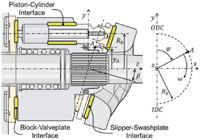
Swashplate-type axial piston machines have found particularly broad use in mobile machinery, agricultural, marine, and aerospace industry due to favorable efficiencies at high working pressures, speeds, and displacements (Ivantysn and Ivantysynova, 2001). In this design of axial piston machines, efficiency is primarily governed by the performance of three lubricating interfaces in terms of piston/cylinder interface, cylinder block/valve plate interface, and slipper/swashplate interface.

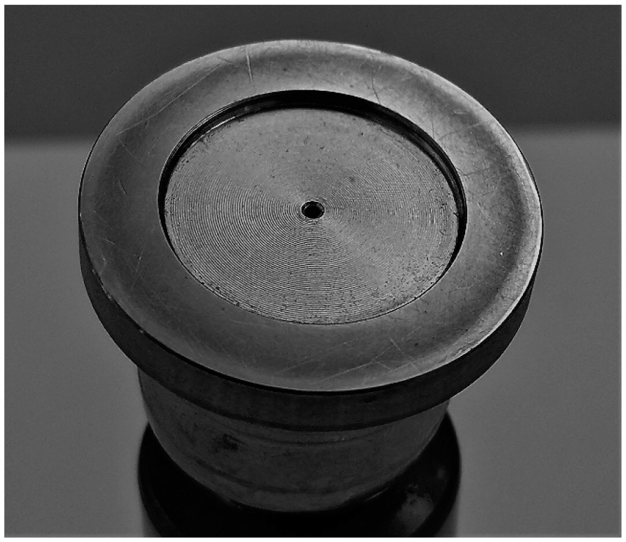
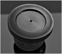
Figure 1 Slipper surface indicating wear on the outside and inside edge of a modern slipper design.

This work focuses on the slipper/swashplate interface illustrated in Figure 1. The slipper mainly serves as a hydrostatic bearing to allow the piston to move along the inclined swashplate surface. A high-pressure fluid film in the slipper/swashplate interface separates the solid bodies. The fluid pressure is created by two sources. Hydrostatic pressure is provided to the slipper pocket from the displacement chamber through a series of channels in the piston/slipper assembly. Separately, hydrodynamic pressure develops in the interface because of the unparalleled surface boundary and the relative macro and micromotion between the slipper and the swashplate. The energy efficiency of slipper/swashplate interface is a function of viscous power loss in the fluid film, which mainly comes through two sources. First, viscous friction dissipates energy due to slipper/swashplate relative motion. Second, the interface represents a leakage path for fluid to travel from the slipper pocket to the case.

An optimal slipper design should minimize energy dissipation while maintaining a stable fluid film to prevent contact and/or wear of machine components. Traditional design methods involve analytical and experimental investigation of prototype slippers.

Modern design approaches incorporate computational modeling into the development process. Yet, modern designs fail to prevent wear-in and contact as can be seen in Figure 1 which shows a slipper profile that has gone through a run-in process starting from a flat profile. Shiny parts of the surface are indication of wear on the slipper surface. Accounting for wear-in and zero-contact design is neglected by past published works. The aim of this paper is to provide means to design a slipper profile that prevents solid to solid contact during steady-state operation while minimizing energy dissipation through the use of an optimization tool coupled with FSTI (Fluid-Solid-Thermal Interaction) model developed by Schenk (2014).

As for the modeling of lubricating interfaces, Shute and Turnball (1958, 1962, 1964) were able to come up with an analytical model for only hydrostatic operation and measure fluid film thickness under the slipper. They continued their work for different operating conditions and different working fluids. Independently, Iboshi and Yamaguchi conducted experimental measurements and analytical models to predict them (1982, 1983). Hooke and Kakoullis (1980) with all the computing advances published comparisons of different numerical models predicting experimental measurements. Before their work, analytical models were developed by use of truncated series. They instead used finite difference method for the Reynolds equation and looked at hydrodynamic pressure and film thickness for centrally loaded slippers (1988). Harris, Edge, and Tilley (1995) came up with a dynamic model of the slipper swashplate that predicted tilt, lift, and effects of slipper contact with swashplate. Later on, Manring and Johnson (2002) found that concave deformations are optimal for stationary bearing with parallel surfaces and their analytical work was modified for the stationary case of slipper-swashplate interface with experimental measurements of pressure (2004). Wieczorek and Ivantysynova (2002) added temperature effects to a model that predicted solid body motion coupling the Reynolds equation. Later on, Huang and Ivantysynova (2003) added solid body pressure deformation (EHL) to the previous model for the piston-cylinder interface. More recently, Schenk put together a fully coupled lubrication model that included thermal effects, pressure deformation, and micromotion of slipper which is the basis for this work. He was able to validate his model through on-line measurements of film thickness.

Iboshi (1986) studied the relationship between power loss and the slipper size assuming uniform clearance between the slipper and the swashplate. He proposed a method for designing a slipper to minimize the power loss while realizing the bearing operation in this paper. Hargreaves (1991) studied how load-carrying ability of slider bearings is affected by adding waviness to the surface of the bearings and concluded that waviness enhances the bearing’s load-carrying ability. Koc, Hooke, and Li studied the effects of flatness of the slipper profile in 1992 and concluded that non-flatness is required for proper operation of slipper. Rasheed (1998) studied the effects of surface waviness on plain cylindrical sliding element bearing and concluded that load capacity of the bearing increases by adding waviness to the bore. Rasheed also concluded that increasing the amplitude of the waves made the increase in load capacity more pronounced. Borghi et al. (2009) studied the influence of different slipper surface profiles on the slipper/swashplate interface performance using a numerical model.Their numerical model assumes rigid body and iso-thermal condition.

Chacon in a more recent study done in 2014 on cylinder block /valve plate interface of axial piston machines, it was concluded that surface shaping for this interface could reduce energy dissipation up to 40% in low pressure and low speed while staying almost the same at high pressure.

The goal of the work presented in this article is to fill the field of slipper surface profile study using the latest multi-domain and multi-physics simulation tool. The simulation tool used in this work considers the non-isothermal thermo-elasto-hydrodynamic effect in the slipper/swashplate interface. The detail explanation of the simulation tool can be found in the chapter following the introduction. The optimal slipper profile that is found in this study is very different than what previous works suggested. The difference mostly due to the consideration of slipper pressure deformation. The design variables, the procedure of finding the optimal slipper profile, and the resulting slipper profile, and its performance are reported in Chapter 3, followed by the findings and discussion in the conclusion chapter.

Fluid-Structure-Thermal Interaction Model for the Slipper/Swashplate Interface

Swashplate-type axial piston machines are comprised of piston/slipper assemblies rotating around an inclined swash plate. The rotating assemblies are constrained by the cylinder block shown in Figure 2 with pitch radius, R_B. A complete description of machine operating principles and kinematics is available in existing literature (Ivantysn and Ivantysynova, 2001). This work focuses on the slipper/swashplate interface, which functions as a load-adaptive fluid film bearing.

The pressure in the interface must balance downward force from displacement chamber pressure, as well as inertial and friction forces. Balance is achieved by the slipper/swashplate interface dynamically adjusting fluid film thickness to match the applied loads. As stated in the literature review, the composite numerical model described here was developed primarily by Schenk (2014). The structure of the model is summarized in Figure 3 and explained in details.

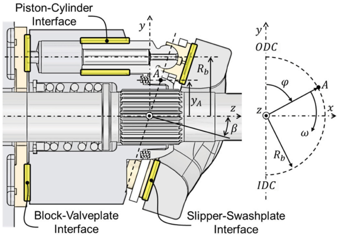
Figure 2 Axial piston machine section view.

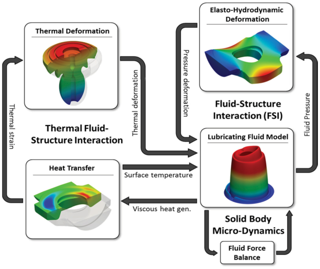
Figure 3 Lubrication model Schenk (2014).

Fluid Model

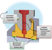
The fluid interacting with the slipper is modeled using a combination of distributed, lumped, and constant parameter domains, as shown in Figure 4. The most critical domain is the fluid beneath the slipper lands.The pressure distribution in the thin film is determined from solving the Reynolds lubrication equation on a 2D grid:

$$\nabla \cdot \left[-\frac{\rho h^3}{12\mu }\nabla \text{p}\right]+\nabla \cdot \left[\frac{\rho h}{2}({\mathit{\upsilon }}_t+{\mathit{\upsilon }}_b)\right]+\rho {\mathit{\upsilon }}_b\cdot \nabla h_b-\rho {\mathit{\upsilon }}_t\cdot \nabla h_t+\frac{\partial }{\partial t}(\rho h)=0.$$

(1)

At any location on the slipper sealing land, h is the gap height between the slipper and swashplate, p is the fluid pressure, ρ is the fluid density, and μ is dynamic viscosity. Subscripts t and b denote top and bottom surfaces, respectively (Schenk, Predicting lubrication performance between the slipper and swashplate in axial piston hydraulic machines, 2014). Once a converged solution of Equation (1) is obtained, the 3D fluid velocity distribution is a simple algebraic result of the fluid pressure distribution and surface velocities.

$$\mathit{\upsilon }=\frac{1}{2\mu }[z^2-(h_t+h_b)z+h_t{h}_b]\nabla p+z\left(\frac{{\mathit{\upsilon }}_t-{\mathit{\upsilon }}_b}{h_t-h_b}\right)+\frac{{\mathit{\upsilon }}_b{h}_t-{\mathit{\upsilon }}_t{h}_b}{h_t-h_b}.$$

(2)

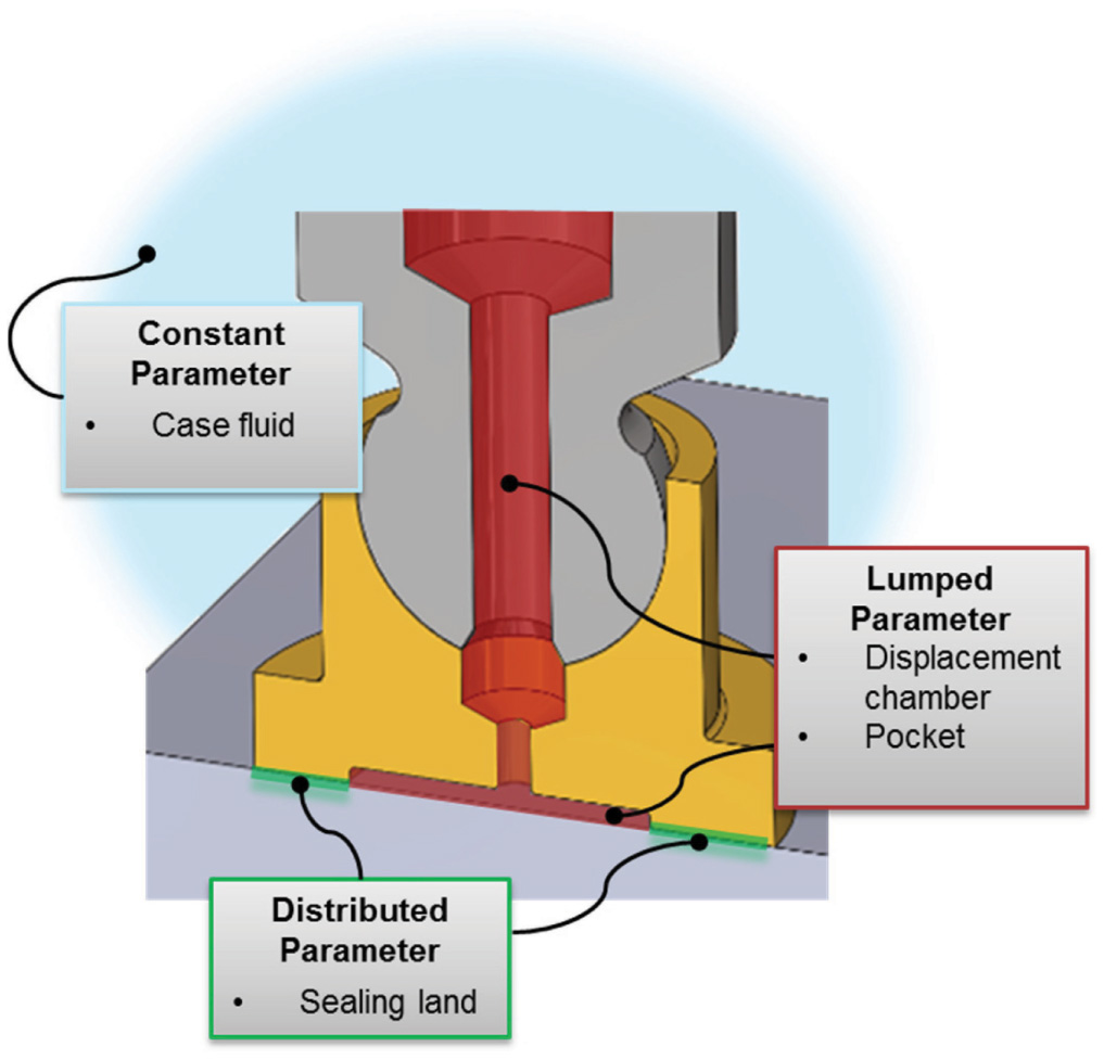
Figure 4 Slipper fluid domains.

Velocity gradients create viscous friction, which dissipates energy as heat. The amount of heat generated is proportional to fluid viscosity.

The viscous dissipation relevant for lubrication neglects terms with derivatives in the flow directions $\left(\frac{\partial }{\partial r},\frac{\partial }{\partial \theta }\right)$.

$$\dot{E}=\mu {\Phi }_{\text{d}}=\mu \left[{\left(\frac{\partial {\mathit{\upsilon }}_r}{\partial z}\right)}^2+{\left(\frac{\partial {\mathit{\upsilon }}_{\theta }}{\partial z}\right)}^2+\frac{4}{3}{\left(\frac{{\mathit{\upsilon }}_r}{r}\right)}^2+{\left(\frac{{\mathit{\upsilon }}_{\theta }}{r}\right)}^2\right].$$

(3)

With energy dissipation and thermal boundaries known, the thin film temperature distribution is found by solving the convective-diffusive energy equation:

$$\nabla \cdot (\rho c_p\mathit{\upsilon }T)=\nabla \cdot (\lambda \nabla T)+\mu {\Phi }_d,$$

(4)

where T is distributed 3D fluid temperature, c_p is fluid heat capacity, and λ is fluid thermal conductivity. The other fluid domains in Figure 4 are necessary as boundary conditions for the distributed parameter models. Case pressure and temperature provide an outer boundary for the interface fluid, while pocket pressure and temperature (p_G, T_G) provide an inner boundary. Pocket pressure varies significantly over the course of a shaft revolution, primarily due to cyclic displacement chamber (DC) pressure. Note that DC pressure is “constant” from the perspective of a single FSI (Fluid-Solid interaction) iteration. It is held constant while instantaneous pocket and sealing land pressures are iterated. Then the simulation advances to the next time-step and DC pressure is updated from off-line data.

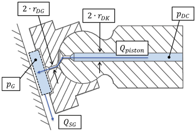
Figure 5 Orifice and pocket pressure model.

One can calculate p_G as the time integral of flows through the pocket control volume boundaries, multiplied by bulk modulus over volume. The resulting pressure bounds the sealing land’s inner radius.

$$\frac{d{p}_G}{\mathit{dt}}=\frac{K}{V_{\mathit{pocket}}}\left(Q_{\mathit{piston}}-Q_{\mathit{SG}}-\frac{{\mathit{dV}}_{\mathit{pocket}}}{\mathit{dt}}\right).$$

(5)

The flow (Q_piston) through the piston/slipper assembly is modeled as passing through a series of turbulent orifices (Schenk, 2014). (Figure 5 using pocket pressure control volume.)

Solid Body Deformation Model

Solid body deformation is a function of fluid pressure, thermal expansion/contraction forces, and constraint boundary conditions. Fluid pressure is calculated from the Reynolds equation, causing local deformation on the lubricating gap surfaces. Thermal expansion forces act on the solid bodies to create additional deformations. Lastly, slipper deformation is constrained at its boundary with the piston ball joint.

A finite element implementation of the elasticity equation (∇ · σ + b = 0) is used to calculate slipper/swashplate deformations due to pressure and thermal loads. The Galerkin formulation of the equation is

$$-{\displaystyle {\int }_{\Omega }}\overline{u}(\nabla \cdot \sigma +b)d\Omega =0,$$

(6)

where ū is a weighting function, σ is the stress tensor at any arbitrary point in a solid, b represents field forces, and the entire solid volume domain is Ω. Conceptually, the solution objective is the minimization of elastic and field potential energies throughout the solid body. An open-source conjugate gradient solver is used to solve a discretized formulation of Equation (6) for nodal displacements.

Solid Body Heat Transfer Model

Solid body temperature is a function of average external heat fluxes, which are applied to all surfaces of a solid body. The lubricating gap temperature distribution is known from the calculation of the convective-diffusive energy equation described previously. Because the fluid temperature is nonuniform, a heat flux exists where it meets the solid body. The instantaneous flux magnitude is $q_{\mathit{gap}}\mathit{ }=\mathit{ }{\lambda }_{\mathit{oil}}\frac{\partial T}{\partial z}$. Outside the lubricating gap, the flow field numerics are too computationally expensive for online calculation. Instead, average convection coefficients are calculated using off-line CFD software. This “mixed” boundary condition is represented by q_mixed = h(T_bulk −T_surf), where the convection coefficient (h) is a function of fluid velocity near the solid body surfaces. With all external temperature gradients available, solid body temperature is found by solving a discretized form of the diffusive heat equation:

$${\displaystyle {\int }_{\Omega }}\overline{u}(\nabla T)d\Omega =0,$$

(7)

throughout the body volume. In Equation (7), ū is a weighting function, T is nodal temperature, and Ω represents the entire solid volume domain. A Gauss-Seidel solver iteratively determines nodal temperatures by minimizing the global squared error between Equation (7) and discrete temperatures integrated over every element. A more complete description of discretization, constraints, and solution technique is included in Schenk’s dissertation (Schenk, Predicting lubrication performance between the slipper and swashplate in axial piston hydraulic machines, 2014).

Rigid-Body Dynamics Model

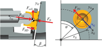
The slipper/swashplate interface functions as a load-adaptive bearing. It achieves load balance through a combination of solid body translation, rotation, and deformation, thereby modifying the fluid film in response to applied load (F_SK). Changes to the fluid film affect the fluid pressure distribution via Equation (1). Area-integrated pressure yields the force (F_fz) and moments (M_fx, M_fy) input to slipper rigid-body dynamics model. Secondary effects from inertia (F_ωG, M_ωg), spring hold-down (F_HD), and viscous friction (F_TG, M_TG) are also considered.

The dynamics model allows three degrees of freedom for micro-motion. Referencing Figure 6, the slipper can translate along the z_G axis, or rotate (tilt) about the socket center. Rotation is constrained by the spherical socket geometry. The equations of motion for the slipper are:

$$\begin{array}{r}\hfill F_{\mathit{fz}}-F_{\mathit{SK}}-F_{\mathit{HD}}=0\\ \hfill M_{\mathit{fx}}+M_{\omega x}=0\\ \hfill M_{\mathit{fy}}+M_{\mathit{TG}}=0\end{array}$$

(8)

The reason right hand side of Equation (8) is set to zero is due to the fact that mass of slipper-piston assembly is small relative to the forces and moments slipper experiences. As described previously, a converged solution to the slipper dynamics problem is achieved iteratively. A Newton-Raphson technique solves for rigid body velocities which satisfy each degree-of-freedom in Equation (8) within a specified error tolerance (Schenk and Ivantysynova, Design and Optimization of the Slipper-Swashplate Interface Using an Advanced Fluid Structure Interaction Model, 2011, NCFP). Once solid body velocities are determined, new slipper positions are calculated by the time-integration of velocity via an Adams-Moulton implicit method. The solution proceeds for several shaft revolutions until steady-state operation is achieved.

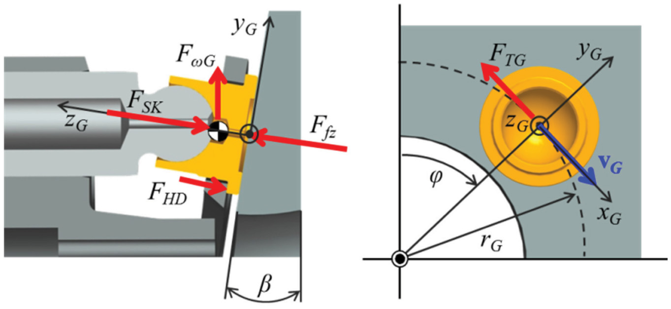
Figure 6 Slipper coordinate system and forces.

Optimization

As mentioned in the state of the art section, Hooke and Kakoullis (1983) concluded that a non-flat (convex) slipper surface geometry results in better hydrodynamic effects. The objective of this optimization is to find a slipper running surface shape that eliminates contact between slipper and swashplate during steady-state operation of the axial piston machine for multiple operating conditions while minimizing energy loss due to leakage and viscous friction.

Design Parameters

To analyze the effects of the slipper surface geometry on the performance of the slipper-swashplate interface, a mathematical expression for the slipper surface geometry is needed. Due to the nature of the slipper-swashplate interface, the slipper surface geometry is chosen to be axis-symmetric. The mathematical expression should be simple (as few variables as possible) and inclusive to account for as many possible designs.

Since the aforementioned model is complex and computationally expensive (∼10 hours for 5 revolutions on a Core i7-4770 @ 3.4 GHz), optimization schemes require large number of simulations (a few thousand potentially) such as NSGA-II andAMGA2 were not really an option. Furthermore, there is only one objective and one constraint which eliminates the need to use algorithms developed mainly for multi-objective optimizations. Also, the goal of this proposed work is demonstrating the influence of the simulation fidelity on the slipper profile study instead of proposing a complex optimization algorithm. For this work, a modified full-factorial optimization was developed. In this scheme, optimization starts from a full factorial optimization on the first operating condition and based on the constraint, keeps reducing the designs that failed to meet that constraint for further operating conditions, leading to fewer simulations.

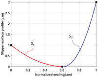
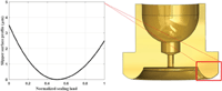
To parametrize the curved slipper surface shape, a simple while inclusive mathematical expression is used. Ageneric sample of slipper surface geometry is depicted in Figure 6. There are three dots at sealing land (SL) = 0, SL = 0.6, and SL = 1. The profile consists of two quadratic curves, one is from SL = 0 to SL = 0.6 (red) and the other from SL = 0.6 to SL = 1 (blue) and for each quadratic equation there are three known boundary values to satisfy a fully defined quadratic equation:

$$\begin{array}{l}{\text{S}}_1={\text{a}}_1{\text{x}}^2+{\text{b}}_1\text{x}+{\text{c}}_1\hfill \\ {\text{S}}_2={\text{a}}_2{\text{x}}^2+{\text{b}}_2\text{x}+{\text{c}}_2\hfill \end{array}$$

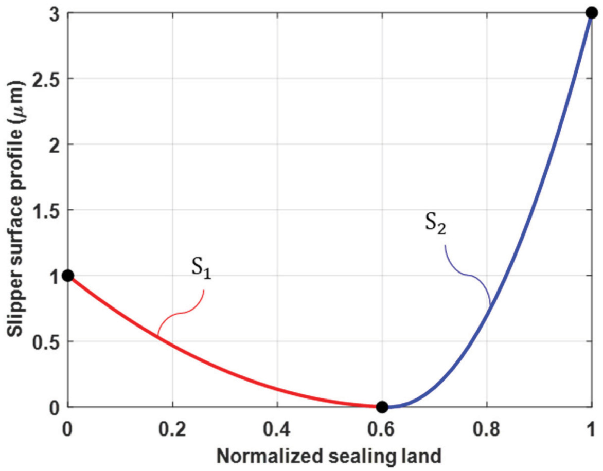
Figure 7 A sample of profile with V0 = 2, V1 = 4, X0 = 0.6.

where a, b, and c are coefficients for each spline and the slipper surface geometry is the combination of these two splines. Therefore, the profile S can be defined using three variables V0 (value of the curve at SL = 0), V1 (value of the curve at SL = 1), X0 (where curve hits 0 height), and the assumption that the slope is zero at the curve’s minimum point.

With only three variables to carry out the optimization, a full-factorial study will be less time-expensive. There are six operating conditions that are used to test the designs in more extreme conditions.

The constraint of the optimization is to simulate no contact between slipper and swashplate during any point of operation. The occurrence of contact is determined whenever the minimum film thickness is lower than a pre-defined value depending on the roughness of the slipper and swashplate surfaces. The optimization function is power loss. For designs that pass the constraint, the best design has the lowest power loss.

Variables and Optimization Scheme

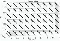
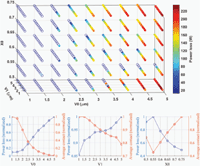
Variables V0, V1, and X0 are chosen according to Figure 8:

V0 and V1 start from 1 micron because all of the designs with V0 or V1 lower than 1 micron did not pass the constraint of the optimization. Furthermore, V0 and V1 are bounded by 5 microns to eliminate the unnecessary function evaluations unfavorably high energy loss due to leakage. It should be noted that an increase in film thickness can reduce power loss at lower film thickness values due to viscous friction forces being dominant. Similarly, for the limits of X0, values below 0.5 fail to pass the optimization’s constraint and X0 values above 0.75 create a sharp edge in the slipper profile for certain designs that should be avoided.

Table 1 Operating conditions used in this study

	dp(bar)	n(RPM)	Displacement(%)
Opcon1	450	600	100
Opcon2	450	3600	100
Opcon3	100	3600	100
Opcon4	450	600	20
Opcon5	450	3600	20
Opcon6	100	3600	20

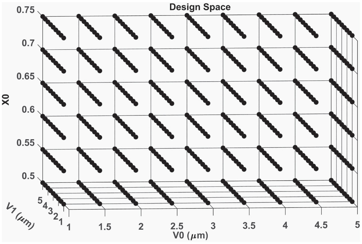
Figure 8 Variable bounds in the optimization. Each of the 486 dots represents a design for opcon1.

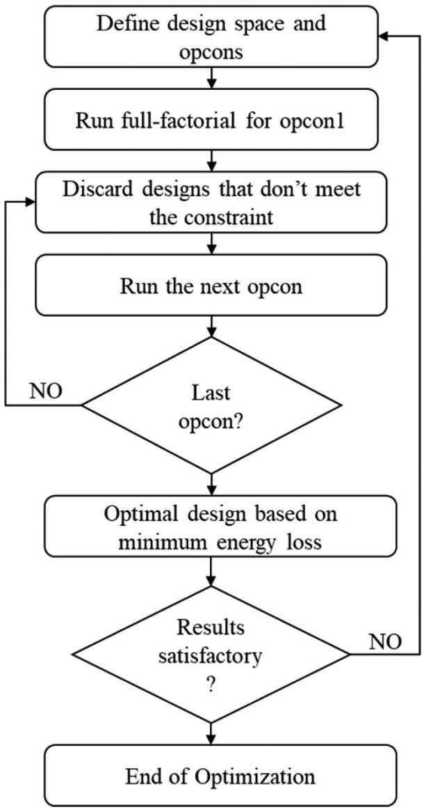
Figure 9 Optimization flow chart.

Out of all the operating conditions, opcon1 is the most prone to showing contact since it has the highest operating pressure and displacement (load) with the lowest speed (hydrodynamic effect). Aflow chart of the optimization scheme is shown in Figure 9.

Results and Discussion

Specifications of the simulated unit are presented in Table 2. The results presented in this paper are for an axial piston pump of swashplate type. The results have not been confirmed for a motor.

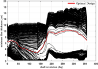
The optimization started with 486 designs for a 75 cc/rev commercial unit at opcon1 and 267 designs passed the no-contact constraint. The minimum film thickness in the last revolution of all 486 designs is roughly presented in Figure 10.

Table 2 Specifications of the simulated unit

Parameter		Value	Unit
Displacement		75	cc/rev
Flow at rated speed		270	l/min
Torque at maximum displacement (theoretical)		1.19	N.m/bar
Speed
	Minimum	500	rpm
	Rated Speed	3900	rpm
	Maximum	4250	rpm
System Pressure
	Max working pressure	450	bar
	Max pressure	480	bar
	Min low loop pressure	10	bar

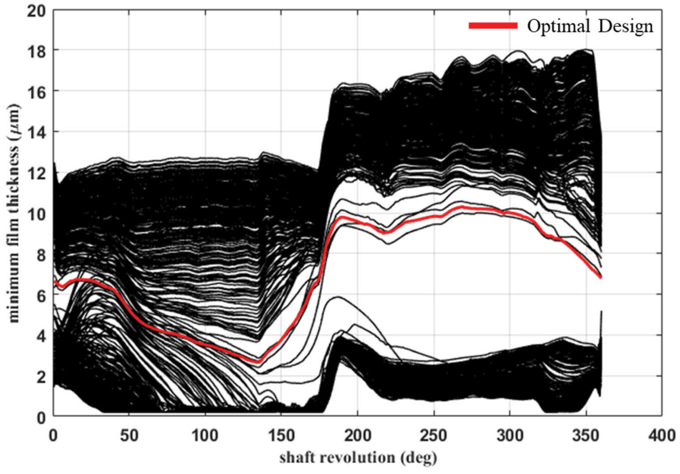
Figure 10 Minimum film thickness of all designs in opcon1.

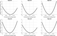
The designs that show minimum film thickness of close to 0 are experiencing contact and hence are eliminated. The optimal design in this set of designs (shown in red) doesn’t show any contact and has the lowest average power loss over the whole shaft revolution. There are a few designs that have lower film thickness during the low pressure stroke, but they show higher film thickness values during the high pressure stroke which contributes more to the power loss. The optimal slipper profile for each operating condition is presented in Figure 11.

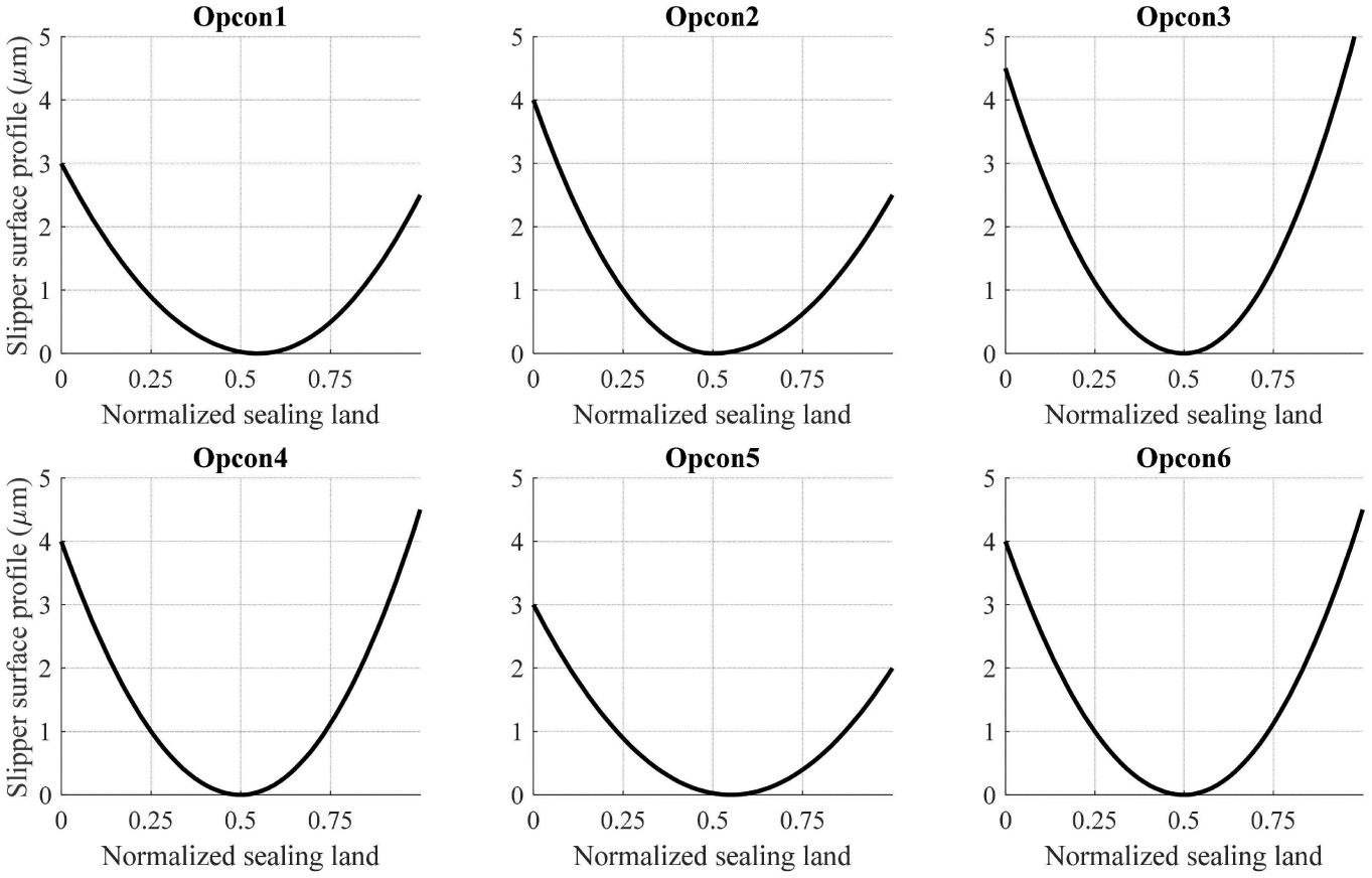
Figure 11 Optimal design for each operating condition.

A comprehensive demonstration of the effect of each of the three design variables V0, V1, and X0 on power loss for opcon1 is presented in Figure 12. The empty markers show designs that were eliminated due to the presence of contact. As value of V0 increases, less contact and more power loss are observed. This is due to the fact that as V0 is increased, film thickness in the inner sealing land region increases which prevents contact in that prone-to-contact region. Once the contact is prevented, increasing the value of V0 will eventually make leakage more dominant than viscous friction which increases power loss. Increasing the value ofV1 also causes less contact and more power loss, however the impact of changing V1 is less than V0 in both contact and power loss as it can be seen from the plots of Figure 12. As for the changes in X0, contact reduces from 0.5 to 0.55 but it increases thereafter. Power loss, on the other hand, increases from 0.5 to 0.55 and then decreases afterward.

Similar patterns are observed for other operating conditions. The optimal designs for other operating conditions are pressented in Table 2.

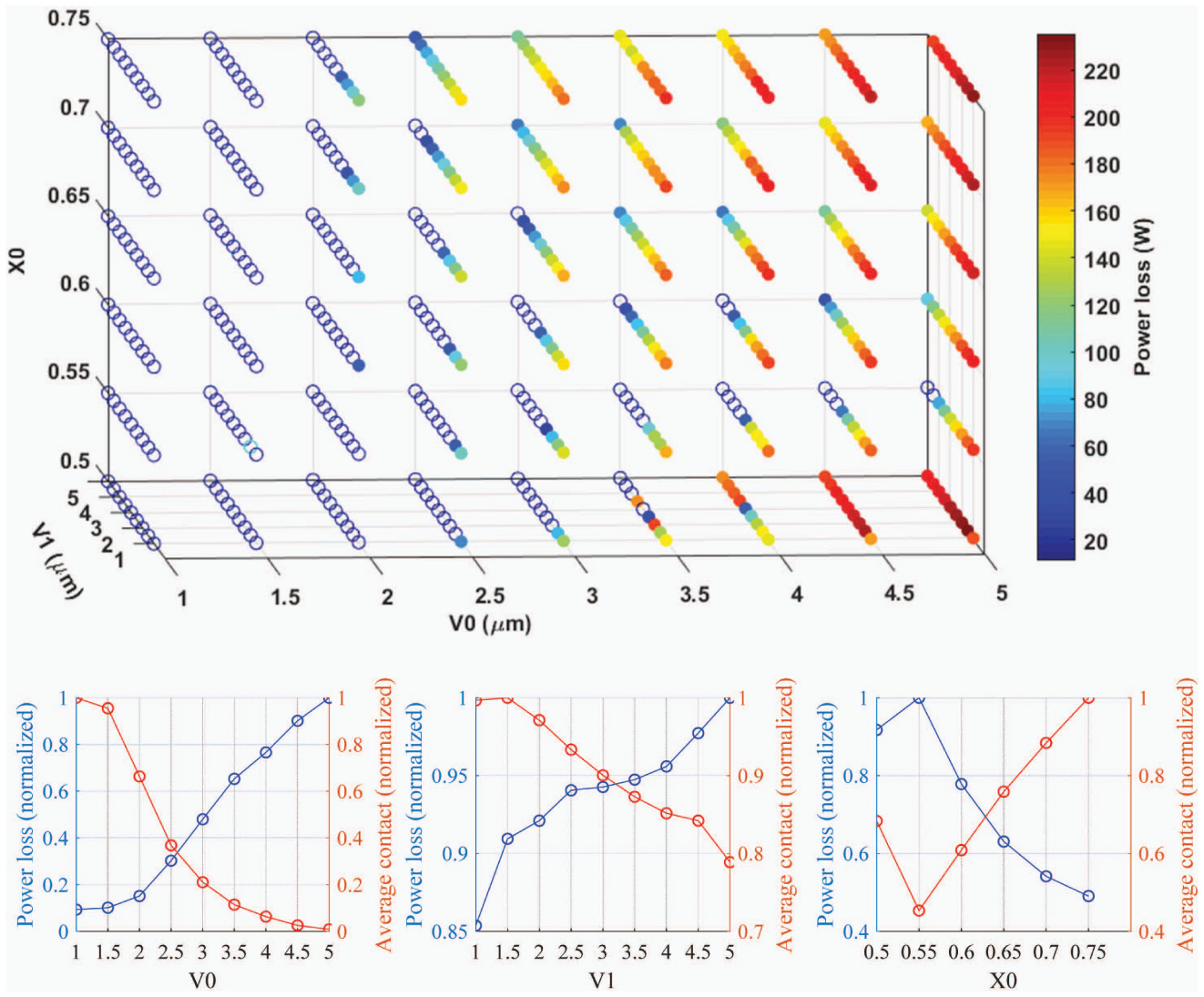
Figure 12 Power loss and contact with respect to optimization variables for opcon1.

Based on the information presented in Table 2, the optimal design to go through all these operating conditions can be found. By finding the overall power loss of common designs over the six operating conditions, the optimal design was found to be 3.5 μm offset at the dc end, 2.5 μm at the case end with the minimum of the curve at the center of the sealing land. The 3D sketch of the slipper shown in Figure 13 is meant for clarification of how the slipper profile would be implemented on the actual slipper part and is not up to scale.

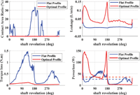
The comparisons that are shown in Figures 14 and 15 involve contact area ratio, leakage, torque loss due to viscous friction forces, and total power loss for opcon1 and opcon2. The contact area ratio is based on the area of fluid film that is lower than the surface roughness to the total area. It needs to be mentioned that total power loss is only accurate for simulations with no contact. When contact is present in simulation, power loss is more than what is presented since power loss due to asperity contact isn’t considered in the physics model. For opcon1, there is major contact during high pressure stroke for the flat profile. Contact is also present during the end of low pressure stroke for the flat profile. Due to the flat profile having lower minimum film thickness during high pressure stroke, leakage is lower than the optimal profile case, however this causes a higher velocity gradient resulting in an increase in torque loss for the flat profile. Although torque loss is high for the flat profile, due to minimal leakage, power loss of the two cases is similar. Opcon1 is an operating condition that a flat slipper design will fail to separate the swashplate and slipper almost throughout the operation. However, this advantage is counteracted by an increase in leakage since the slipper runs at higher film thickness during operation. For the flat profile, 7.6% of slipper’s surface area experiences contact with swashplate on average. One possible reason for the collapse of flat profile during low pressure stroke could be due to lack of a converging physical wedge in the profile and low rotational speed of 600 RPM, resulting in a lack of hydrodynamic pressure build-up. Overall in opcon1 – through the use of slipper surface geometry with v0 of 3 μm, v1 of 2.5 μm, and x0 of 0.55-torque losses were reduced by 87.9% when using the optimal profile compared to the flat one. Due to the increase in leakage in the optimal profile, power loss was improved by only 3.7% overall.

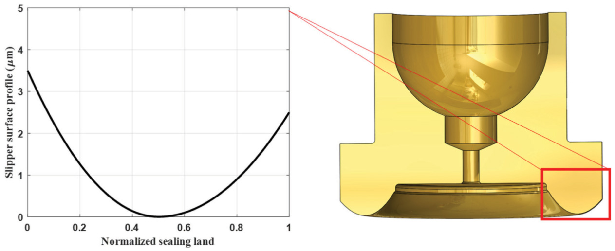
Figure 13 Optimal profile for all the operating conditions.

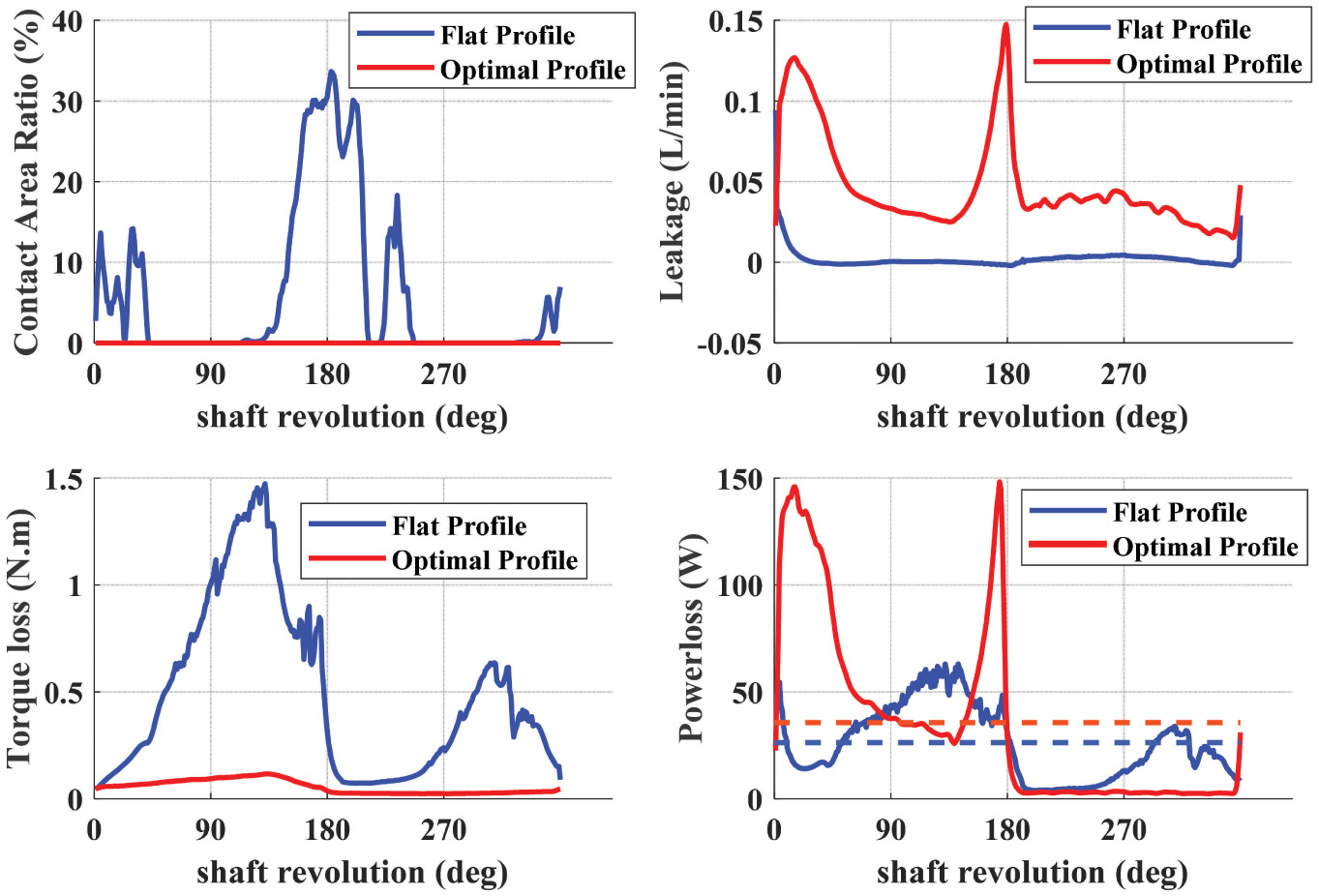
Figure 14 Comparison of performance of a single slipper between optimal design from opcon1 and a flat profile.

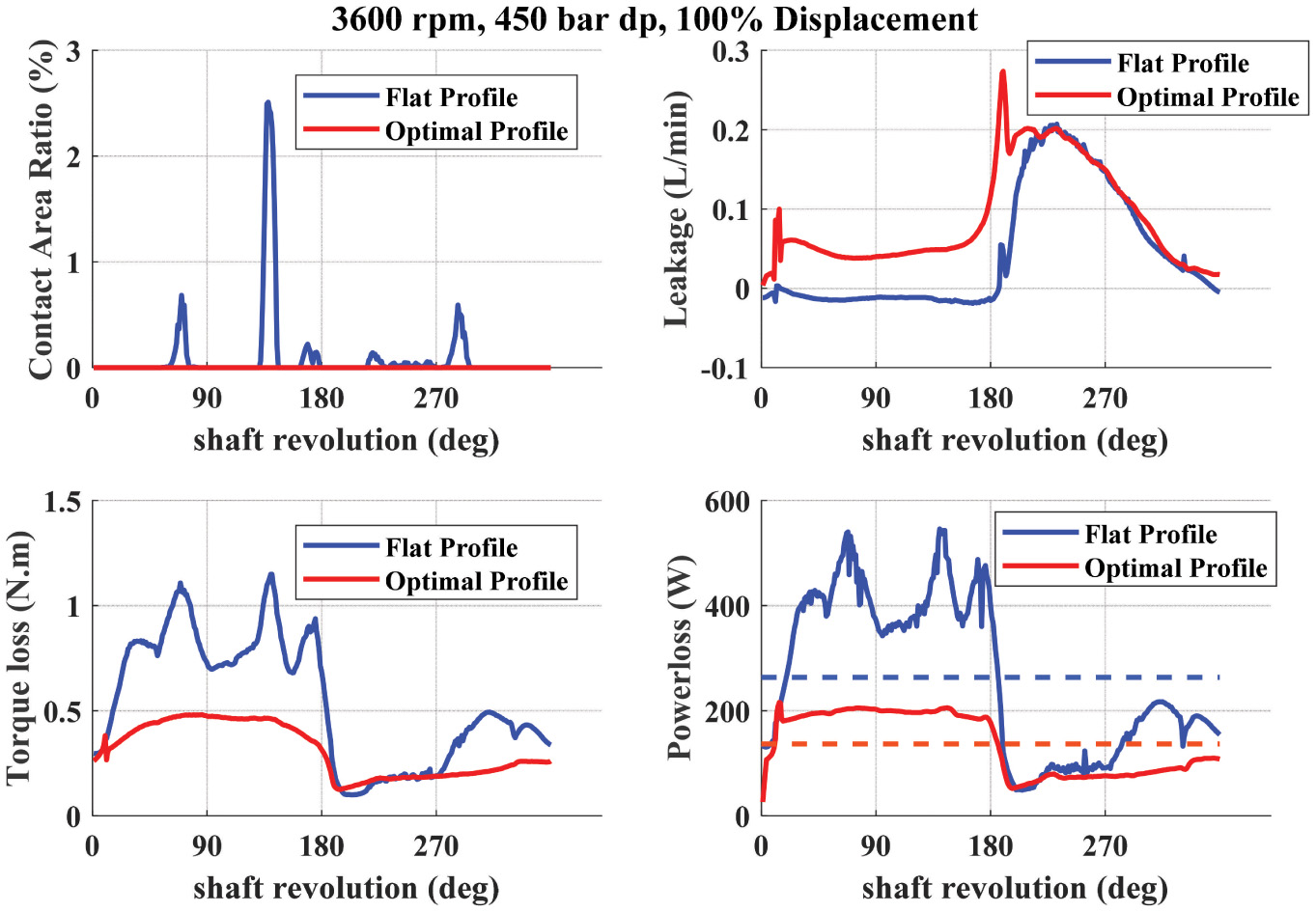
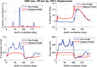
Figure 15 Comparison of performance of a single slipper between optimal design from opcon2 and a flat profile.

As for opcon2, same trends are observed. The primary difference between flat and optimal profile for this operating condition is in the high pressure stroke. The optimal profile shows clear improvement in overall power loss for opcon2. In opcon2, the flat profile shows less contact than opcon1, and shows more lift during low pressure stroke than opcon1. In opcon2- using a slipper surface geometry with v0 of 4 μm, v1 of 2.5 μm, and x0 of 0.5-torque loss was reduced by 47.7%, leakage was doubled, and power loss was reduced by 49.2%.

Table 3 Comparison between the optimal profile and the flat profile

	dp (bar)	n(RPM)	Displacement (%)	Total Designs	Passed Designs	V0	V1	X0
Opcon1	450	600	100	486	267	3	2.5	0.55
Opcon2	450	3600	100	267	39	4	2.5	0.5
Opcon3	100	3600	100	39	38	4.5	5	0.5
Opcon4	450	600	20	38	37	4	4.5	0.5
Opcon5	450	3600	20	37	32	3	2	0.55
Opcon6	100	600	20	32	32	4	4.5	0.5

Table 4 Comparison between the optimal and flat profile for all opcons for a single slipper

	450 bar, 600 rpm, 100% Disp. (#1)		450 bar, 3600 rpm, 100% Disp. (#2)		100 bar, 3600 rpm, 100% Disp. (#3)
	Flat	Optimal	Flat	Optimal	Flat	Optimal
Leakage (lpm)	0.00	0.07	0.04	0.07	0.05	0.10
Torque loss (N.m)	0.52	0.04	0.51	0.36	1.33	0.29
Power loss (W)	27.33	51.89	239.20	145.41	555.04	117.74
Contact area ratio (%)	6.75	0	0.13	0	4.21	0

	450 bar, 600 rpm, 20% Disp. (#4)		450 bar, 3600 rpm, 20% Disp. (#5)		100 bar, 3600 rpm, 20% Disp. (#6)
	Flat	Optimal	Flat	Optimal	Flat	Optimal
Leakage (lpm)	0.287	0.332	0.055	0.259	0.053	0.204
Torque loss (N.m)	0.022	0.021	1.358	0.326	0.853	0.268
Power loss (W)	221.10	253.9	487.81	231.3	344.78	110.5
Contact area ratio (%)	0	0	4.87	0	1.42	0

Table 3 shows a comparison between the optimal profile (Figure 13) and a flat profile for all operating conditions in Table 1. This comparison is for a single slipper design that runs through all the operating conditions. The optimal profile shows the most amount of improvement in operating conditions 3 and 6. In opcon1 and opcon4, the optimal profile is showing an increase in power loss. In opcon1, there is a large amount of contact for the flat profile making the optimal profile the better choice, however in opcon4, there is no advantage in using the optimal profile since none of the profiles show any contact. Opcon4 is a very unusual operating condition and is included for the sake of completeness. In low speed, high pressure, and partial displacement conditions, it seems that convex profiles are not needed since the slipper tends to lift more due to low swashplate inclination. For high speed conditions, the convex profiles show a clear improvement that explains their hydrodynamic characteristics. On average, there is a 51.4% improvement in power loss for the six operating conditions. Similarly, the results of a commercial profile are shown in Table 4.

Conclusion

In summary, this research has shown that modifications to the slipper surface geometry can significantly impact the performance of the slipper-swashplate lubricating interface in axial piston machines. The results of this paper indicate that full film lubrication during steady state operation is achievable by changing the slipper surface geometry. It is also shown that the performance of the slipper-swashplate interface is very sensitive to the changes to the slipper surface geometry. Based on the comparison between flat and optimal shown in this paper for operating conditions of 450 bar pressure difference, 600 rpm of speed, and 100% displacement, the optimal slipper surface geometry reduces torque loss by 87.9% and improves power loss by 3.7%. For the operating condition of 450 bar pressure difference, 3600 rpm of speed, and 100% displacement, the optimal profile showed an improvement of 47.7% in torque loss and a decrease of 49% in power loss. In a separate comparison between an optimal profile (Figure 13) and a flat profile for all six operating conditions, it was observed that high speed conditions make the best use of convex profiles. Throughout all six operating conditions, power loss was reduced by 51.4% on average.

Comparing to the profiles that the previous works (Iboshi, 1986 and Borghi et al. 2009) suggested, the slipper profile proposed in this paper firstly includes the convex shape along the sealing land edge on the pocket side thanks to the consideration of the slipper pressure deformation. The profile that is found from the reported study is specifically optimized for a 75 cc commercial pump. But the significance of considering the elastic deformation during the slipper profile study is demonstrated.

Nomenclature

cp	Heat capacity	[J/kg · K]
dDG	Slipper orifice diameter	[m]
dK	Piston diameter	[m]
DGout	Slipper outer land diameter	[m]
DGin	Slipper inner land diameter	[m]
FfZ	Fluid pressure force	[N]
FHD	Hold-down force	[N]
FSK	Piston reaction force	[N]
FTG	Viscous slipper friction force	[N]
FωG	Centrifugal slipper force	[N]
h	Fluid film thickness	[m]
n	Shaft speed	[rpm]
p	Fluid film pressure	[Pa]
pcase	Case pressure	[Pa]
pDC	Displacement chamber pressure	[Pa]
pg	Slipper pocket pressure	[Pa]
P	Power	[W]
r	Gap radial ordinate	[m]
QSG	Slipper leakage	[m3/s]
t	Time	[s]
υb, υt	Bottom and top surface velocities	[m/s]
υr	Radial velocity	[m/s]
vθ	Tangential velocity	[rad/s]
z	Gap height coordinate	[m]
αD	Slipper orifice coefficient	[−]
β	Swashplate angle	[%]
λf	Thermal conductivity	[W/m · K
μ	Dynamic viscosity	[Pa · s]
ρ	Density	[kg/m3]
τ	Stress	[N/m2]
φ	Shaft angle	[deg]

References

Bergada, J., Watton, J., Haynes, J. and Davies, D., 2010. “The hydro-static/hydrodynamic behavior of an axial piston pump slipper with multiple lands,” Meccanica, Vol. 45, pp. 585–602.

Borghi, M., Specchia, E. and Zardin, B., 2009. “Numerical analysis of the dynamic behaviour of axial piston pumps and motors slipper bearings”, SAE International Journal of Passenger Cars-Mechanical Systems, 2(2009-01-1820), pp. 1285–1302.

Chacon, R., 2014. Cylinder block/valve plate interface performance investigation through the introduction of micro-surface shaping (Master thesis, Purdue University).

Dhar, S., Vacca, A. and Lettini, A., 2013. “A Novel Fluid-Structure-Thermal Interaction Model for the Analysis of the Lateral Lubricating Gap Flow in External Gear Machines,” in Proc. ASME/Bath Symposium on Fluid Power and Motion Control, Sarasota, FL, Paper No. FPMC2013-4482.

Hargreaves, D. J. 1991. “Surface waviness effects on the loadcarrying capacity of rectangular slider bearings”, Wear, Vol. 145, pp. 137–151.

Harris, R. M., Edge, K. A. and Tilley, D. G., 1996. “Predicting the Behaviour of Slipper Pads in Swash Plate – Type Axial Piston Pumps”, Journal of Dynamic Systems, Measurement and Control, Vol. 118, pp. 41–47.

Hooke, C. J. and Kakoullis, Y. P., 1983. “The effects of non-flatness on the performance of slippers in axial piston pumps.”

Hooke, C. J. and Li, K.Y., 1989. “The Lubrication of Overclamped Slippers in Axial Piston Pumps and Motors – The Effect of Tilting Couples”, Proc. Inst. Mech. Engrs. 203 C, pp. 343–350.

Hyang, C. and Ivantysynova, M., 2003. “A new approach to predict the load carrying ability of the gap between valve plate and cylinder block,” in Bath Workshop on Power Transmission and Motion Control PTMC 2003, Bath, UK.

Iboshi, N., 1986. “Characteristics of a Slipper Bearing for Swash Plate Type Axial Piston Pumps and Motors: 3rd Report, Design Method for a Slipper with a Minimum Power Loss in Fluid Lubrication”, Bulletin of JSME, 29(254), pp. 2529–2538.

Iboshi, N. and Yamaguchi, A., 1982. “Characteristics of a Slipper Bearing for Swash Plate Type Axial Piston Pumps and Motors (1st report, Theoretical Analysis)”, Bulletin of JSME, Vol. 25, No. 210, pp. 1921–1930.

Iboshi, N. and Yamaguchi, A., 1983. “Characteristics of a Slipper Bearing for Swash Plate Type Axial Piston Pumps and Motors (2nd report, Experiment)”, Bulletin of JSME, Vol. 26, No. 219, pp. 1583–1589.

Ivantysn, J. and Ivantysynova, M., 2001. Hydrostatic Pumps and Motor, Principles, Designs, Performance, Modeling, Analysis, Control and Testing, New Delhi: Academic Books International.

Kazama, T. and Yamaguchi, A., 1993. “Application of a mixed lubrication model for hydrostatic thrust bearings of hydraulic equipment,” ASME J. Tribology, Vol. 115, pp. 686–691.

Koc, E., Hooke, C. J. and Li, K. Y., 1992. “Slipper balance in axial piston pumps and motors,” Trans. AMSE, J. Tribology, Vol. 114, pp. 766–772.

Koç, E. and Hooke C. J., 1996. “Investigation Into the Effects of Orifice Size, Offset and Overclamp Ratio on the Lubrication of Slipper Bearings”, Tribology International, Elsevier Science, Vol. 29, No. 4, pp. 299–305.

Koç, E. and Hooke C. J., 1997. “Considerations in the design of Partially Hydrostatic Slipper Bearings”,Tribology International, Elsevier Science, Vol. 30, No. 11, pp. 815–823.

Manring, N. D., Johnson, R. E. and Cherukuri, H. P., 2002. “The Impact of Linear Deformation on Stationary Hydrostatic Thrust Bearing”, ASME J. of Tribol., Vol. 124, pp. 874–877.

Manring, N. D., Wray, C. L. and Dong, Z., 2004. “Experimental Studies on the Performance of Slipper Bearings within Axial Piston Pumps”, ASME J. of Tribol., Vol. 126, pp. 511–518.

Pelosi, M. and Ivantysynova, M., 2012. “Heat Transfer and Thermal Elastic Deformation Analysis on the Piston/Cylinder Interface of Axial Piston Machines,” ASME Journal of Tribology, Vol. 134, pp. 1–15.

Pelosi, M. and Ivantysynova, M., 2008. “A New Fluid-Structure Interaction Model for the Slipper-Swashplate Interface,” in Proc. of the 5th FPNI PhD Symposium, Kracow, Poland.

Rasheed, H. 1998. “Effect of surface waviness of the hydrodynamic lubrication of a plain cylindrical sliding element bearing”, Wear, Vol. 223, pp. 1–6.

Schenk,A., 2014. Predicting lubrication performance between the slipper and swashplate in axial piston hydraulic machines, Ph. D. Thesis, Purdue University.

Shute, N. and Turnbull, D., 1958. “A preliminary investigation of the characteristics of hydrostatic slipper bearings,” BHRA REport RR610.

Wieczorek, U. and Ivantysynova, M., 2000. “CASPAR – A Computer Aided Design Tool for Axial Piston Machines,” in Proc. Bath Workshop on Power Transmission and Motion Control PTMC 2000, Bath, UK.

Wieczorek, U. and Ivantysynova, M., 2000. “CASPAR – A computer aided design tool for axial piston machines” in Proc. Bath Workshop on Power Transmission and Motion Control PTMC 2000, Bath, UK, pp. 113–126.

Zecchi, M. and Ivantysynova, M., 2012. “Cylinder block/valve plate interface – a novel approach to predict thermal surface loads,” Dresden, Germany.

Biographies

Ashkan A. Darbani Born on July 6th 1994 in Mashhad, Iran. He received his B.S. degree in Mechanical Engineering from Brigham Young University – Idaho in 2016 and currently pursuing his master’s degree at Purdue University in Mechanical Engineering. His research revolves on modelling and optimization of slipper-swashplate interface of axial piston pumps.

Lizhi Shang Born on March 25th 1989 in Tianjin (China). He received his B.S. degree in Thermal Energy and Power Engineering from Huazhong University of Science and Technology in 2011 and his M.S. degree in Mechanical Engineering in New Jersey Institute of Technology in 2013. He is currently a PhD student at Maha Fluid Power Research Center in Purdue University. His main research interests are modeling and optimizing of hydraulic pumps/motors.

Jeremy R. Beale Born on October 18th 1991 in Chapel Hill, North Carolina. He received his B.S. degree in Mechanical Engineering from the University of Kentucky in 2014 and his M.S. degree in Mechanical Engineering from Purdue University in 2017. He is currently a hydraulic applications engineer at Tec-Hackett Inc. in Fort Wayne, Indiana.

Monika Ivantysynova Born on December 11th 1955 in Polenz (Germany). She received her MSc. Degree in Mechanical Engineering and her PhD. Degree in Fluid Power from the Slovak Technical University of Bratislava, Czechoslovakia. After 7 years in fluid power industry she returned to university. In April 1996 she received a Professorship in fluid power & control at the University of Duisburg (Germany). From 1999 until August 2004 she was Professor of Mechatronic Systems at the Technical University of Hamburg-Harburg. Since August 2004 she is Professor at Purdue University, USA. Her main research areas are energy saving actuator technology and model based optimisation of displacement machines as well as modelling, simulation and testing of fluid power systems. Besides the book “Hydrostatic Pumps and Motors” published in German and English, she has published more than 80 papers in technical journals and at international conferences.

International Journal of Fluid Power, Vol. 20_2, 245–270.
doi: 10.13052/ijfp1439-9776.2025
©2019 River Publishers

Abstract

Introduction

Fluid-Structure-Thermal Interaction Model for the Slipper/Swashplate Interface

Fluid Model

Solid Body Deformation Model

Solid Body Heat Transfer Model

Rigid-Body Dynamics Model

Optimization

Design Parameters

Variables and Optimization Scheme

Results and Discussion

Conclusion

Nomenclature

References

Biographies