Adaptive Identification and Application of Flow Mapping and Inverse Flow Mapping for Electrohydraulic Valves
Jianbin Liu, André Sitte and Jürgen Weber*
Institute of Mechatronic Engineering – Chair of Fluid-Mechatronic Systems,
Technical University of Dresden, Germany
E-mail: jianbin.liu@tu-dresden.de; andre.sitte@tu-dresden.de;
fluidtronik@mailbox.tu-dresden.de
*Corresponding Author
Received 23 September 2021; Accepted 30 September 2021; Publication 12 November 2021
Abstract
Good estimation of flow mapping (FM) and inverse flow mapping (IFM) for electrohydraulic valves are important in automation of fluid power system. The purpose of this paper is to propose adaptive identification methods based on LSM, BPNN, RBFNN, GRNN, LSSVM and RLSM to estimate the uncertain structure and parameters in flow mapping and inverse flow mapping for electrohydraulic valves. In order to reduce the complexity and improve the identification performance, model structures derived from new algorithm are introduced. The above identification methods are applied to map the flow characteristic of an electrohydraulic valve. With the help of novel simulation architecture via OPC UA, the accuracy and efficiency of these algorithms could be verified. Some issues like invertibility of flow mapping are discussed. At last, places and suggestions to apply these methods are made.
Keywords: Identification, flow mapping, inverse flow mapping, electrohydraulic valve, LS, BP, RBF, GRNN, LSSVM, RLS.
1 Introduction
For many years, hydraulic-mechanical control systems have been characterized by extremely high requirements for good operability, high reliability, robustness and a favorable cost-benefit ratio. However, an increase in efficiency and productivity for control systems can only be achieved through the use of electrohydraulic components in combination with electronics, sensors and software. Among the many components that contributed to the success of electrohydraulic control systems, the proportional valve elements are of considerable importance. The flow rate of valves cannot be described precisely enough by simple physics-based equations because of highly non-linear characteristic. Offline-Identification of flow mapping is an efficient way to compensate the complex non-linearity in valves partially. Unfortunately, this method cannot adapt to changes in the system properties over time, e.g., the influences of temperature, erosion on the valve edges and wear of valve spool. Therefore, a self-learning system for adaptive identification of flow mapping for proportional valve elements in electrohydraulic system is crucial, in which not only the complex non-linearity can be compensated, but also the flow mapping can be adapted to the varying system parameters. Numerous system identification methods are now available, but the suitability of adaptive identification for valve elements has not been sufficiently investigated yet. In addition, it is necessary to make a prediction based on limited data about flow mapping in some cases. As for the application of flow mapping, various fields can be found such as demand-based flow rate control for energy-efficient operation, high precision control, autonomous control, maintenance and fault detection, condition monitoring and diagnostics. If the flow rate characteristic relationship Q f (U, p, T…) is inverted to U f (p, Q, T…), the inverted flow mapping could also be used for feedforward control instead of the traditional lookup table method.
Starting with research and comparison of different adaptive identification methods, suitable for an adaptive identification of flow mapping in electrohydraulic valves, considering offline/online-processing capability, signal-to-nosie ratio, model fidelity and so on, different adaptive identification methods based on LSM, BPNN, RBFNN, GRNN and LSSVM are chosen for offline identification and RLSM for online identification of flow mapping of electrohydraulic valves. Examples of adaptive identification with RLSM can be found in the work by Vahidi et al. [1], C. Kamali et al. [2], S. Dong et al. [3] and M. Kazemi et al. [4]. Modern BPNN was first published by S. Linnainmaa in his master thesis [5]. BPNN is a supervised learning neural network, which is one of the most popular NN for approximation. D.J. Jwo et al. [6] have applied the BPNN to geometric dilution of precision (GDOP) approximation. BPNN for 2-D GDOP and weighted GDOP approximation can also be found in works by C.S. Chen [7, 8]. O. Nelles et al. [9] presented a comparison between RBF networks and classical methods for identification of nonlinear dynamic systems. RBFNN has wide applications in many areas such as computer science, aircraft and mathematics [10–14]. The comparison among BPNN, RBF and GRNN for function approximation could be found in [15, 16]. The application of LSSVM for classification and regression has been proposed by [17–19].

Figure 1 Combination of source data types for identification [22].
Besides the identification methods, the source data types play an important role in identification. Figure 1 proposes different source data types for identification. Static data are time independent. On the contrary, dynamic data are time dependent and inertial effects have to be taken into account. The transition data type between them are quasi-static data, which are time dependent but slow enough to neglect its inertial effects. Usually, structured data characterize the flow behavior of throttle valves. These data are determined at discrete input signals, representing the operating range. There is a high resolution along the x-axis, whereas only a few data point exist along the y-axis. The data-gap increases the requirements for the training procedures (optimization) and eventually creates great deviations between model and estimation. A comprehensive scatter data-set appears to be advantageous in terms of coverage. However, arbitrary data is difficult to interpret and to evaluate, which is why the use of such data is not very widespread. Limited and noisy flow data are more common. The restrictions mostly result from limited capacities of the test rig or system setup. Noise is inherent to measurement data, which requires filtering of data or smoothing capabilities of the approximation procedures. Operating point data contain operating points resulting from a typical working cycle of machine. In this paper, quasi-static data combined with structured data and scattered data are used for identification.
The subsequent paper is organized as follows: In Section 2, to be acquainted with the static characteristics of the electrohydraulic valve, a test rig in laboratory has been set up. After that, a virtual demonstrator with real-time and streaming OPC UA data has been implemented, which was carried out in simulation environment to validate the adaptive parameter identification methods. Then the suitable adaptive identification methods are chosen and derived in Section 3, including LSM, BPNN, RBF, GRNN, LSSVM and RLSM. After that, the previously developed adaptive identification methods have been applied in order to obtain the evolving flow mapping (FM) and inverse flow mapping (IFM) of a piloted proportional valve. The results demonstrate that the adaptive identification methods have convincing performance for the flow mapping (FM) and inverse flow mapping (IFM) of electrohydraulic valves. In Section 4, the previously developed flow mapping (FM) and inverse flow mapping (IFM) have been applied in order to enhance the control performance and robustness of system. Finally, conclusions are drawn and some issues to be solved are discussed in Section 5.
2 Modelling and Test Rig of Electrohydraulic Valve
2.1 Modelling of Electrohydraulic Valve
Figure 2 shows the construction of a proportional seat valve also known as “Valvistor”, which is based on hydraulic position feedback.
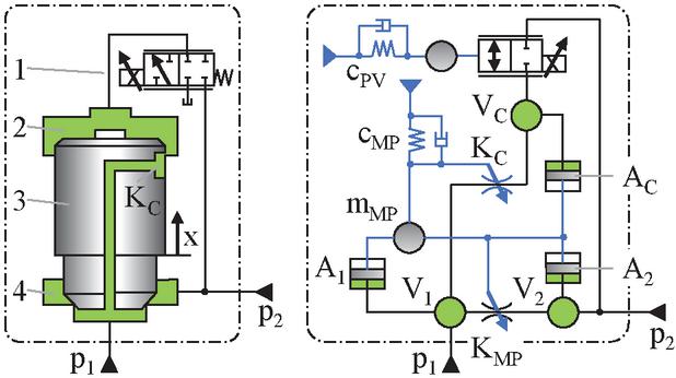
Figure 2 Construction for flow direction p to p (left)/simplified simulation model structure (right) [22].
Due to a negative overlap of the variable orifice between control chamber (2) and main poppet (3), the pressure in the control chamber is equal to the pressure at the valve inlet . Because the upper area of the main poppet is greater than the area facing , the closing position of seat valve is ensured. Opening the pilot valve (1), pressure drop creates the pilot flow and reduces the control pressure in the control chamber. The main poppet starts moving until the equilibrium of forces is established. Neglecting flow- and friction forces and rearranging the force balance equation for the main poppet leads to:
| (1) |
The flow rate across control-orifice results in:
| (2) |
Where x is the displacement of main poppet and is the negative overlap. According to Equations (1) and (2), the following interrelation can be obtained:
| (3) |
The flow rate across main poppet is given by:
| (4) |
Neglecting the negative overlap in Equation (3) and substituting Equation (3) into Equation (4), results in following equation:
| (5) |
The total flow rate is given by:
| (6) |
From Equations (5) and (6), it can be seen that Valvistor amplifies a small flow rate through the pilot valve, which is similar to a transistor. Therefore, the name “Valvistor” is derived from valve and transistor. More about the Valvistor can be found in [20, 21] and [22].
2.2 Test Rig and Results
Figure 3 shows the hydraulic plan and corresponding test rig built in laboratory. It consists of a hydraulic reservoir, an adjustable pump, a pressure relief valve, a test valve (Valvistor), a pressure control valve (load valve) and a cooling system, which is not shown here. The instrumentations installed in the system are various pressure sensors, temperature sensor, a flow meter and displacement sensor, which is responsible to measure the displacement of main poppet. For the static measurements, the hydraulic system could be seen as constant pressure system with p bar. Because of limited power of pump, max. flow rate is restricted to Q l/min. Furthermore, in order to reduce temperature fluctuation and latency, the oil temperature is measured inside the tank instead of at the test valve outlet in ISO 4411. Another advantage of using tank temperature is the ability to reduce renovation costs and temperature sensors in multiple actuators system. To acquire the static characteristics of the electrohydraulic valve, the tank temperatures and the control signals for test valve are given in the manner of discrete values. At the same time, with the help of load valve, the outlet pressure varies between maximum and minimum so that the flow rate through test valve is changed in a quasi-static manner.
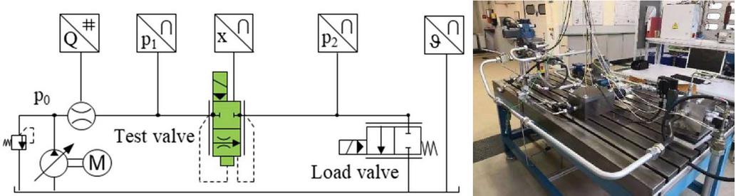
Figure 3 Hydraulic plan for test rig (left)/ Test rig in laboratory (right).
Figure 4 presents the flow rate-pressure drop characteristic curves of test valve at different control voltages and constant tank temperature (C) on left side. On right side is the flow rate characteristic is plotted against temperature at different control voltages and a constant pressure drop (). As a whole, the simulation results are in good agreement with the measured results. Based on the validated model, it’s convenient to apply the adaptive identification methods in next section.
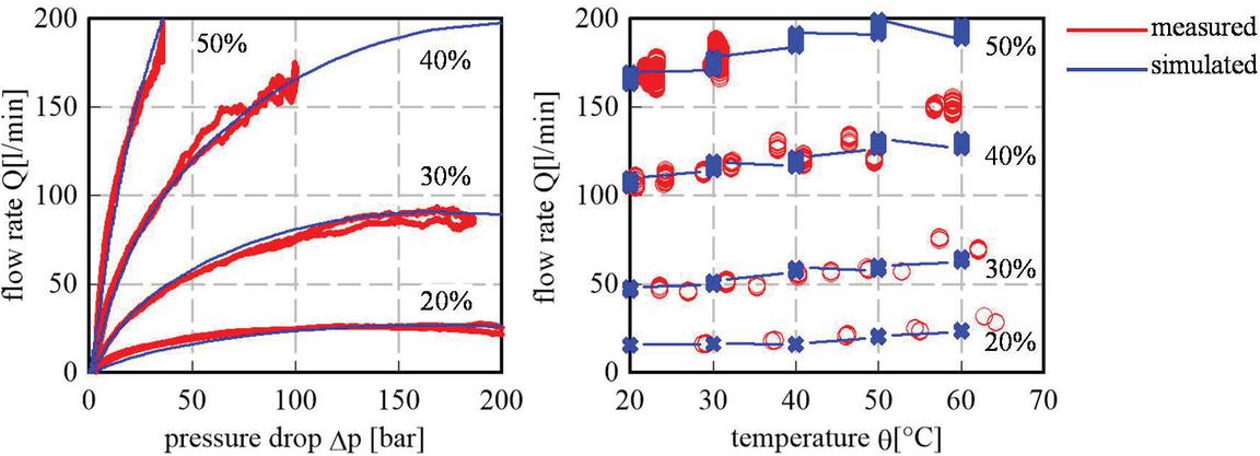
Figure 4 Flow rate – pressure drop characteristic curves at different control voltages and C (left)/flow rate – temperature characteristic curves at different control voltages and bar (right).
2.3 Simulation Test
With the help of software-in-the-loop (SIL) testing, the developed identification algorithms and control strategies could be tested within virtual environment. Compared with hardware-in-the-loop (HIL), SIL is a useful tool to ensure the more efficient software development at earlier stages. It is not necessary to consider the expensive hardware and physical interfaces. Figure 5 depicts the MATLAB-SimulationX Co-Simualtion via an OPC UA coupling layer. The coupling layer is not only responsible for exchange of process variables and time synchronization between controller and simulation model, but also for the data exchange between host PC or Cloud and lower embedded system.
As is well known, model identification consists of model structure identification and model parameter identification. In general, the change of system structure is very slow, for example, the erosion in electrohydraulic valve. Therefore, the offline identification could take place in host PC or Cloud, which need much computational effort and storage space but less real-time requirement, especially for the model structure identification. The online identification and controlling mission would be implemented in lower embedded system, which could meet the requirement of real-time but suffer from the lack of computational effort and storage space. In particular, it is of great significance for model parameter identification which needs to be running constantly in real time. By this way, it’s easy to solve real-time, computational effort and storage problem at the same time. Because almost all the Clouds in the market that support OPC UA are not free, the offline identification could only be carried out in a host PC for this paper. After the definition of the interface, all the relevant input/output signals between virtual controller, simulation model and host PC are exchanged via OPC UA Server. The UaExpert is designed as an OPC UA viewer, which supports OPC UA features like browsing OPC UA address space, reading and writing of variable values and UA attributes, monitoring of data changes and events.
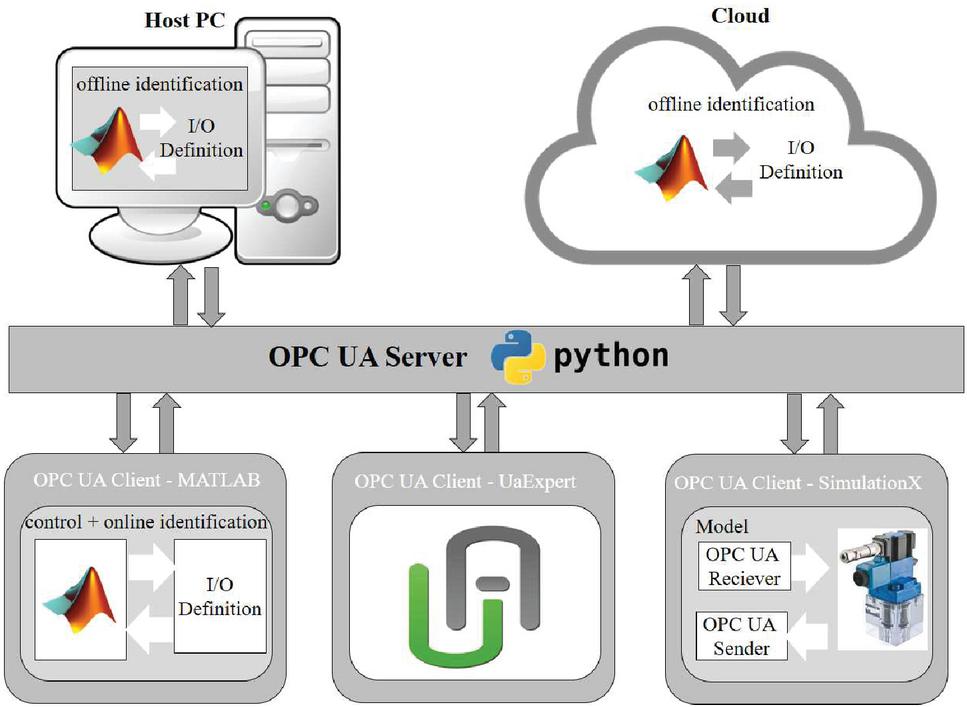
Figure 5 MATLAB-SimulationX Co-Simulation via OPC UA.
3 Adaptive Identification Algorithm
3.1 Outline of Adaptive Identification
Figure 6 shows the simplified basic sequence of the identification.

Figure 6 Basic sequence of the identification [23].
The first step is to define the purpose of identification. The purpose of this paper is to identify the relationship among flow rate , control voltage , pressure drop and temperature for electrohydraulic valves. In other words, the objective is to identify flow mapping (FM) and inverse flow mapping (IFM) . With the help of a priori knowledge, it can be presented in Figure 7.
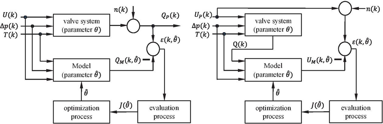
Figure 7 Identification for flow mapping (left)/ Identification for inverse flow mapping (right).
The next step is the determination of model structure. Model structure identification is based on the purpose of identification and the application of mathematical models in practice. Most of the mathematical model structures of linear systems can be easily identified by input and output data. However, since the static characteristics of electrohydraulic valves are more complex, which contain strong nonlinear factors, prior knowledge, assumptions and experiments have to be included in the determination of model structure. Based on these, there are two ways to determine the model structure.
The first way is to linearize the nonlinear system at first. Then use the linear system identification methods. This method will be adopted with LSM in the next step. According to Taylor’s theorem, the following Algorithm 1 show the procedure to find optimal approximation for the Valvisor valve‘s structure:
Algorithm 1 Linearization of model structure for flow mapping identification
1: Input:
2: Control voltage ; pressure drop ; tank temperature ; flow rate Q
3: max. Order of Control voltage ;
4: max. Order of pressure drop ; max. Order of tank temperature ;
5: Output:
6: Model Criterion
7: Model Terms
8: Normalization
9: LOOP Process
10: for :1:
11: for :1:
12: for :1:
13: ;
14: for :1:
15: for :1:
16: for :1:
17: n n1; C(n, 1) i; C(n, 2) j; C(n, 3) k; JK1% calculate order matrices C
18: end for
19: end for
20: end for
21: for :1:
22: for :1:
23: X(k, i) U(k)C(i, 1)* C(i,2)* T(k)C(i,3); JK1% generate new inputs X
24: end for
25: end for
26: Y Q;
27: use LSM to fit the data (X, Y) and calculate the significance level of all terms X(k, i), according to the t-test
28: filter the terms X(k, i) which are not significant at the 5% significance level
29: replace X and generate new inputs XX whose terms are complete significant
30: use LSM to fit the data (XX, Y) and calculate model criterion AICc
31: store the index for terms which are significant
32: end for
33: end for
34: end for
35: find the min. value in model criterion AICc and the corresponding index.
36: at last, get the optimal polynomial for model
For simplicity, a lot of codes are not shown in algorithm. It is worth mentioning that the information criteria for model selection, e.g., Akaike information criterion (AIC), Bayesian information criterion (BIC), corrected AIC (AICc) and consistent AIC (CAIC). Because AIC tends to overfit in small data set. Corrected AIC (AICc) is adopted in algorithm for better performance in small samples. More information about criteria for model selection can be found in [24–27]. Pressure drop is replaced by in algorithm. The reasons for that are closer to the theoretical flow rate formula and a kind of simple and efficient order-reduction means. By means of this linearization, it can greatly expand the scope of identification methods. Then the system approximation can be simplified as:
| (7) |
where is the estimated parameter and is the new input whose terms are complete significant.
The second method is to directly identify the nonlinear system model structure. For certain types of nonlinear systems, models can be formulated that match well with the requirements on the model structure of known identification methods [23]. A nonlinear system identification using different neural network will be covered in the following.
The following task is the application of suitable identification methods to identify model parameters. By means of a weighted point evaluation on the basis of the criteria suitability for linear or nonlinear processes, allowable signal-to-noise ratio, suitability for offline or online processing, ability for time variant system and resulting model fidelity, preferred adaptive identification methods could be determined. At the end, LSM (Least Squares Method), BPNN (Back-Propagation Neural Networks), RBFNN (Radial basis function Neural Network), GRNN (General regression Neural Network) and LSSVM (Least-Squares Support-Vector Machine) are chosen for offline identification and RLSM (Recursive Least Squares Method) for online identification of flow mapping of electrohydraulic valves.
3.2 Offline-Identification Methods
A complete derivation of all considered identification methods would go beyond the scope of this paper. Therefore, a selection of algorithms is explained in the following subsections. More Information about offline identification methods please to refer to [1–19].
3.2.1 Non-recursive least squares method (LSM)
The non-recursive least squares method (LSM) can be utilized for linear systems. In general, the model estimation for electrohydraulic valves is given as:
| (8) |
The error between measured output and model estimation is determined as:
| (9) |
At different time steps , it is easy to get the measured inputs and output , which can be noted as and . Similarly, the error can be defined as . Then the system equations can be written as:
| (10) |
If the vector and are defined as and , the system equation can be reduced to matrix form:
| (11) |
If the vector , and are defined as , and , the system Equations (10) can be reduced to matrix form:
| (12) |
Where is the parameter vector, which is to be identified.
According the principle of least square, the cost function:
| (13) |
To compute the minimum of cost function, the first derivative with regard to the parameter vector is set to zero:
| (14) |
This equation can be solved to provide an estimation for parameter vector as:
| (15) |
Where L is the length of data.
3.2.2 Radial basis function neural network (RBFNN)
RBFNN has recently drawn much attention due to their good generalization ability and a simple network structure that avoids unnecessary and lengthy calculation as compared to the multilayer feed-forward neutral network (MFNN). RBFNN has three layers: the input layer , the hidden layer and the output layer , which are shown in Figure 8.
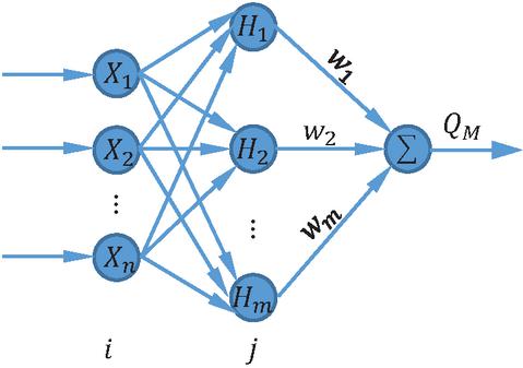
Figure 8 Typical RBFNN structure [28].
The input vector and radial basis function vector in RBFNN are defined as: and with and . Where is the Gaussian function value, which is given as:
| (16) |
Where is the center vector of neural net and is the width of Gaussian function for neural net . The width vector of Gaussian function can be given as . Furthermore, the weight vector is given by .
The output of RBFNN is a linear combination of the Gaussian function values:
| (17) |
The cost function of RBFNN can be defined as:
| (18) |
3.2.3 Results analysis and verification of offline identification
The last step is the performance evaluation of the identified methods, the so-called verification by comparison of measured plant output ( or ) and predicted model output ( or ). In order to identify the parameters of the electrohydraulic valve, following structured data in Figure 9 are used. To get the system excited enough, the signals cover the whole operating range U [0, 100] %, p [0, 200] bar and T [20, 60]C.
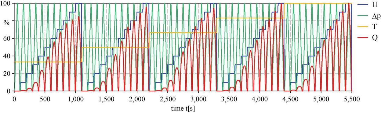
Figure 9 Process of structured data to identify.
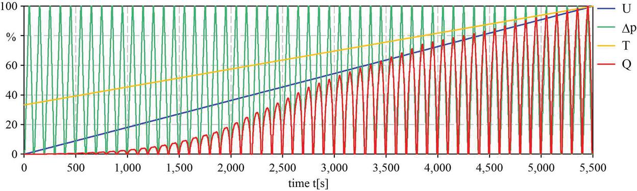
Figure 10 Process of test data to identify.
In order to identify the parameters of the electrohydraulic valve, the scattered data can also be utilized. For a better comparison, structured data in Figure 9 could be randomly distributed and be approximately used as scattered data.
In order to illustrate the merit of the above-mentioned methods, it is appropriate to use the test signals in Figure 10 for verification. The test data include data that does not exist in the training data.
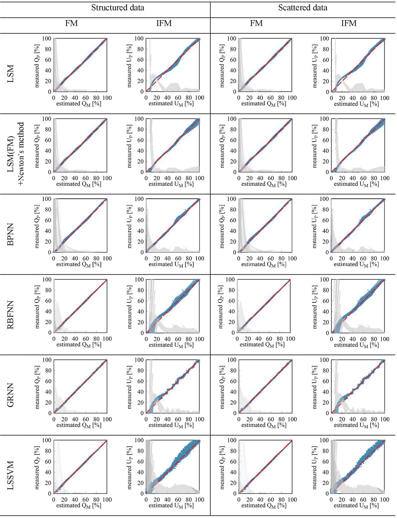
Table 1 shows verification of different identifications with structured data and scattered data. In order to compare the performance of identification for the different methods, the estimated flow rate is plotted against the measured plan flow rate (or the estimated voltage is plotted against the measured plant voltage ) from test data. With an ideal identification, all points would lie exactly on the 45 red diagonal curve. The relative errors are plotted in grey color and calculated from:
| (19) |
It could be found in table that all identification methods show almost the same results for structured data and scattered data. That is to say, the data types are insensitive to the selected offline identification methods. Additionally, a conclusion can be drawn that all identification methods show a good approximation for flow mapping (FM). However, compared with the flow mapping identification, all identification performances decrease for inverse flow mapping (IFM), which can be deduced from the grey area in diagram. There are two main reasons for that one is stronger nonlinearity for IFM and the other is the irreversibility in IFM. To illustrate this, look at the flow rate equation in Equation (20) for electrohydraulic valves:
| (20) |
As the pressure drop and flow rate approach zero at the same time, zero divided by zero is going to come up. The corresponding case in reality is that there are no flow rate and pressure drop or a little, but the input voltage for valves could be arbitrary in working area. In order to get better performance for identification, it’s necessary to filter the data in small pressure drop area with threshold value . It depends not only on the operating rage of the valve but also on the signal-to noise ration of signals. The only way to determine this threshold value is by trial and error. The threshold value for IFM identification in Table 1 is set to 9 bar. In the identification methods listed in table, BPNN presents the best approximation results, especially in IFM. Unlike RBFNN and GRNN, BPNN with multiple hidden layers can achieve a better nonlinear mapping. LSSVM not only has the worst results but also needs the most computational efforts. In the case of large data set, it’s best to avoid using LSSVM. According to the verification results, BPNN will be preferred in use-cases with low real-time requirements and high-performance computers, e.g., machine tool, thermoforming machine. But for mobile machines, an implementation of neural network algorithms in embedded systems could be problematic, since massive floating-point calculations are inevitable, which require much computational efforts and storage space. It can be seen in table that LSM could also reach the comparable identification goodness with neural networks. In particular, LSM can be adopted for FM identification at first and then newton’s method can be used to find the numerical solution for IFM. If LSM is replaced with RLSM, it’s possible to run on an embedded system with real-time requirements.
3.3 Online-Identification Methods
3.3.1 Recursive least squares method (RLSM)
The precondition for non-recursive least squares method (LSM) requires all the measured data had first been stored then estimates the parameter in one pass. Such a method requires a lot of computational efforts, especially the matrix inversion in (15). Therefore, the non-recursive least squares method (LSM) is not suitable for real time identification. In order to overcome these deficiencies, recursive least squares method (RLSM) is introduced.
Table 1 Verification of Identification with structured data and scattered data
Furthermore, with appropriate modifications and forgetting factor, it’s easy to realize the adaptive identification and solve the data saturation problem at the same time. With
| (21) |
The following equation can be given:
| (22) |
In order to reduce the error in matrix inversion of , according to matrix inversion lemma:
The Equation (22) can be given as:
| (23) |
Where is the gain vector:
| (24) |
Together with Equations (23) and (24), one then obtains:
| (25) |
According to the definition of and , the Equation (15) can be transformed as:
| (26) |
Base on Equation (22), one can substitute in Equation (26) and obtains
| (27) |
Which combined with (25), one can write:
| (28) |
From Equations (23), (24) and (28), recursive least squares method (RLSM) can be descripted by:
| (29) |
If the estimation parameters of an electrohydraulic valve change abruptly, for example, damage of valve, RLSM can’t capture the new values in time. The estimation parameter from RLSM will vary continuously but slowly, this is co called data saturation. With some modification, RLSM can be changed to RLSM with forgetting factor, in which less weight is given to older data and more weight to recent information. With new definition:
Where is the forgetting factor and . The Equation (21) can be modified as:
| (30) |
Thus, it follows:
| (31) |
If one substitutes the Equation (31) in Equation (29), RLSM with forgetting factor is given as:
| (32) |
Table 2 Verification of RLSM () with structured data and scattered data

3.3.2 Results analysis and verification of online identification
For a better comparison, the same training data and test data already applied in the previous methods are used for online identification. Table 2 shows verification of RLSM () with structured data and scattered data. In general, RLSM with these two data types show suitable identification results. Compared with scattered data, RLSM with structured data can achieve the same accuracy at the end, although the rate of convergence is slow. Without consideration for difficulty in data acquisition, methods with scattered data are much faster than methods with structured data in terms of the rate of convergence (less than 100s). Compared to offline method LSM, RLSM not only shows almost the same results regarding accuracy at the end but also more effective. If the forgetting factor is set to 1 (), RLSM with forgetting factor will be degenerated as classical RLSM, which will eliminate the fluctuation. However, classical RLSM deals with all the past data equally and can result in data saturation problem. Therefore, it is necessary to select suitable forgetting factors in practice.
The RLSM can be used only if the model structure is known. In practice, valve manufacturers usually provide measured data for some type of valve, which is sufficient to identify the model structure. Otherwise, it’s reasonable to identify the model structure with offline method and parameters can be estimated online. By contrast, RLSM with forgetting factor is more suitable for real application. At first, RLSM with forgetting factor is able to deal with all kinds of data types. Furthermore, another advantage of RLSM with forgetting factor in contrast to other methods is that it enables to integrate multi-dimensional dependencies with a reduced set of parameters in the software development for embedded systems. Regrading to the fitting quality of RLSM, one way to improve the accuracy is to adopt partition identification for local areas. The second way is to increase order in model structure until the accuracy meets the requirements.
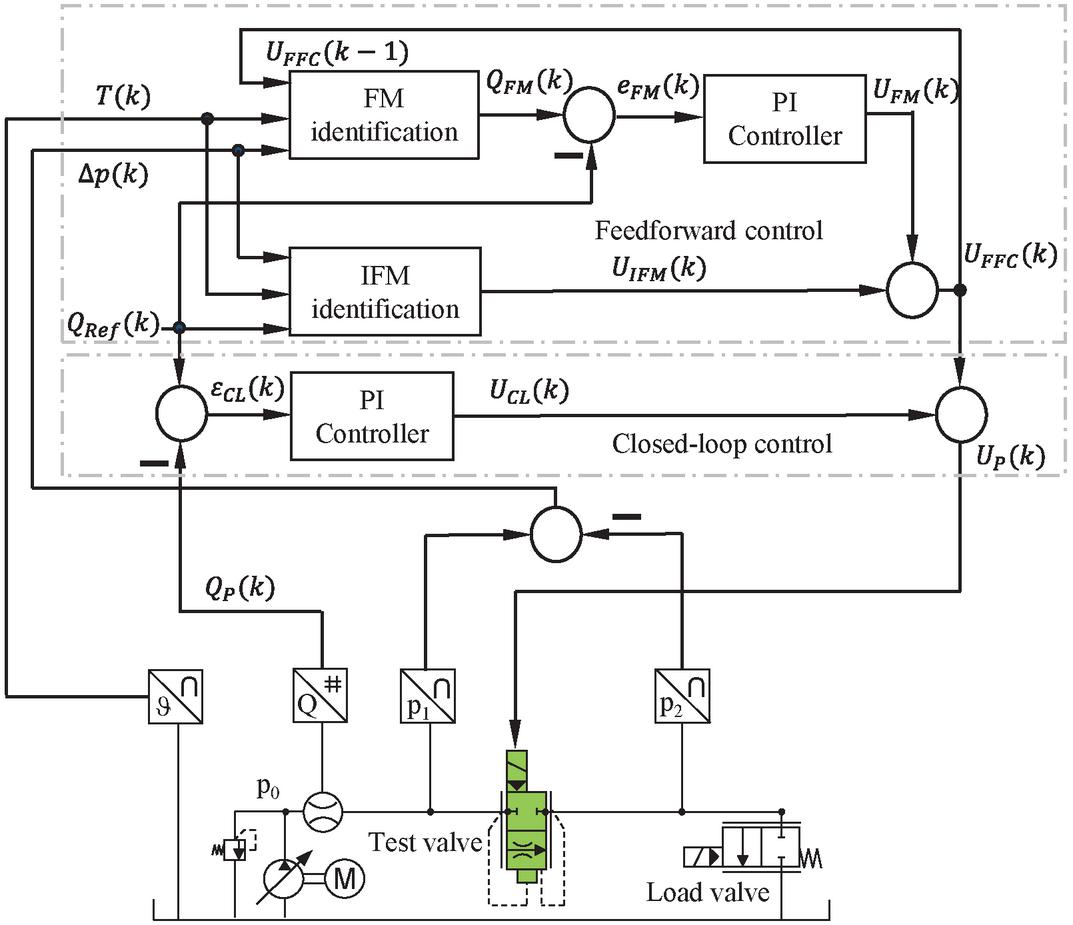
Figure 11 Application of FM and IFM for flow rate control.
4 Application of Flow Mapping (FM) and Inverse Flow Mapping (IFM) Identification
Since the flow rate can be calculate accurately using the measured velocity of cylinder, the flow mapping (FM) and inverse flow mapping (IFM) identification methods can be applied in the flow rate control or velocity control. Therefore, a compound flow rate control is proposed based on the identification methods, and the schematic of the application of FM and IFM is given in Figure 11. The control loop consists of two parts: feedforward control and closed-loop control. The control voltage , pressure drop , together with the temperature and the measured flow rate are given to FM and IFM for the training process. After that, the calculated flow from FM is compared with the reference flow and the error is given to a PI controller to obtain FM voltage . Combined with the IFM voltage , it’s not so hard to get the total voltage for feedforward control. At the same time, the measured flow is also compared with the reference flow and the error is given to another PI controller to obtain closed loop voltage . At last, the feedforward voltage and closed loop voltage build the control voltage for valve together. There are two reasons for using FM in feed forward control: the first reason is that FM is generally more accurate than IFM and the second reason is to compensate for IFM’s irreversibility at small pressure drop (e. g. ). In addition, with the help of condition of monitoring, it is easy to realize redundant control and improve the robustness in system. If the flow rate or velocity transducer fails, the hydraulic system could be still controlled by feedforward control (FM+IFM). If the pressure or temperature transducer fail, the closed loop control (CL(PI)) could ensure controllability for the whole system, although the control performance will be reduced.
Figures 12–14 show the system response under different conditions. As is shown in the figures, flow mapping (FM) inverse flow mapping (IFM) PI controller in closed in loop (CL(PI)) presents the best performance. Conventional PI controller in closed in loop (CL(PI)) can hardly work well at all operating points. Compared with FM, FM IFM can enhance the tracking performance of the output and further reduce the control error. As expected, the FM control can be problematic under the low pressure drop conditions. The controller with Newton’s method (NM) shows worse performance than expected in real time. The reason is that Newton’s method cannot obtain the optimal numerical value in limited sampling time (10 ms) at big step response. Therefore, Newton’s methos should be avoided in practical applications, especially for embedded controller. The results demonstrate that the performance of the controller FM IFM CL(PI) can track the reference input satisfactorily and reduce the settling time.
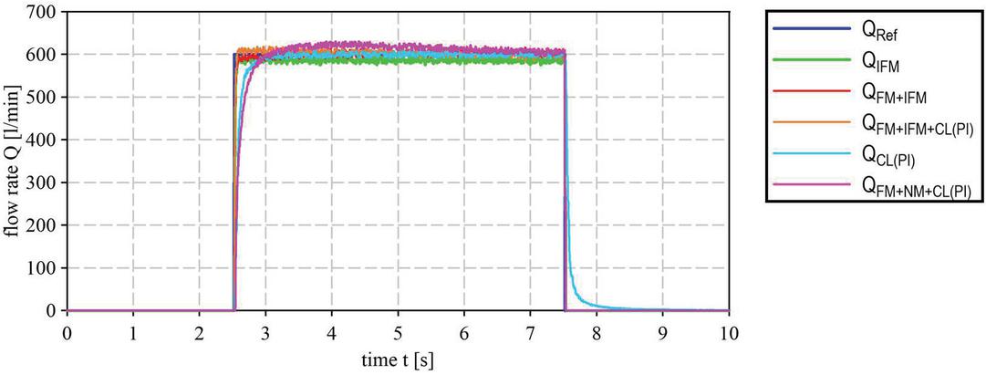
Figure 12 Step response at , , C).

Figure 13 Step response at , , C).

Figure 14 Step response at , , C).
5 Conclusion and Outlook
In this research, different flow mapping identification methods for electrohydraulic valves are proposed. This paper presents an analysis and comparison of different identification methods and data structures for 4D-flow mapping. The proposed methods can be applied to adaptive identification for real machines in the future. Moreover, their identification accuracy and convergence property have been sufficiently investigated.
So far, the flow mapping identification methods have been applied for only one valve with little hysteresis. In order to improve the generalization of the methods and get a more reliable conclusion, the next investigation steps are concerned with the further development of the proposed methods with respect to different types of valves and inclusive hysteresis. After that, the adaptive PI controller with FM and IFM should be further tested.
Nomenclature
| Designation | Denotation | Unit |
| F | Force | N |
| Estimated parameters | – | |
| A | Matrix | – |
| A | Piston area of main poppet in inlet | mm |
| A | Ring area of main poppet in outlet | mm |
| bj | Width vector | – |
| B | Matrix | – |
| c | Parameter in center vector | – |
| C | Matrix | – |
| C | Center vector | – |
| H | Radial basis function vector | – |
| Gaussian function value | – | |
| I | Index | – |
| I | Unit Matrix | – |
| L | Gain vector | – |
| j | Index | – |
| J() | Cost function | – |
| K | Flow coefficient of control-orifice | l/minbarmm |
| K | Flow coefficient of main poppet | l/minbarmm |
| p | Constant system pressure | bar |
| p | Pressure in valve inlet | bar |
| p | Pressure in valve outlet | bar |
| p | Pressure in the control chamber | bar |
| P(t) | Data matrix | – |
| P | Initial data matrix | – |
| Q | Flow rate through valve | l/min |
| Q | Flow rate through control-orifice | l/min |
| Q | Max. Flow rate through main poppet | l/min |
| Q | Estimated flow rate for valve(model) | l/min |
| Q | Flow rate through main poppet | l/min |
| Q | Measured flow rate for valve(plant) | l/min |
| Q | Measured flow rate vector | – |
| Q | Flow rate through pilot valve | l/min |
| Q | Total flow rate through valve | l/min |
| t | Time | s |
| U | Input voltage for valve | V |
| V | Valve chamber in inlet | mm |
| V | Valve chamber in outlet | mm |
| V | Control chamber in valve | mm |
| Weight vector | – | |
| x | Input variable | – |
| x | Displacement of main poppet | mm |
| x | Negative overlap of control-orifice | mm |
| X | Matrix for inputs | – |
| X | Input vector | – |
| Input parameters in input matrix | – | |
| X | Input parameters matrix | – |
| y | Input variable | – |
| Z | Output variable | – |
| p | Pressure drop through valve | bar |
| p | Pressure drop between inlet and outlet | bar |
| p | Pressure drop between inlet and control chamber | bar |
| Error | – | |
| Error matrix | – | |
| Area ratio | – | |
| Temperature | C | |
| Temperature in tank | C | |
| Vector for estimated parameter | – | |
| (t) | Estimated parameter vector in LSM | – |
| Forgetting factor | – | |
| FM | Flow mapping | |
| IFM | Inverse flow mapping | |
| LSM | Least square method | |
| BPNN | Back propagation neural networks | |
| RBFNN | Radial basis function neural network | |
| GRNN | General regression neural network | |
| LSSVM | Least-Squares Support-Vector Machine | |
| RLSM | Recursive least squares method | |
| MFNN | Multilayer feed-forward neutral network | |
| OPC UA | Open Platform Communications Unified Architecture | |
| CL | Closed in the loop |
References
[1] A Vahidi, A Stefanopoulou and H Peng. Recursive least squares with forgetting for online estimation of vehicle mass and road grade: theory and experiments. Mechanical Engineering Dept., University of Michigan, Ann Arbor.
[2] C Kamali, A A Pashikar and J R Raol. Evaluation of recursive least squares algorithm for parameter estimation in aircraft real time applications. Aerospace Science and Technology 15, pp. 165–174, 2011.
[3] S Dong, L Yu, W A Zhang and B Chen. Robust extended recursive least squares identification algorithm for Hammerstein systems with dynamic disturbances. Digital Signal Processing 101, 102716, 2020.
[4] M Kazemi and M M Arefi. A fast iterative recursive least squares algorithm for Wiener model identification of highly nonlinear systems. ISA Transaction, 2016.
[5] S Linnainmaa. The representation of the cumulative rounding error of an algorithm as a Taylor expansion of the local rounding errors. Master’s Thesis, 1970.
[6] D J Jwo, K P Chin. Applying Back-propagation Neural Networks to GDOP. Journal of Navigation, 55, pp. 97–108, 2002.
[7] C S Chen and S L Su. Resilient Back-propagation Neural Network for Approximation 2-D GDOP. Proceedings of the International MultiConference of Engineers and Computer Scientists, Vol II, pp. 1–5, 2010.
[8] C S Chen, J M Lin and C T Lee. Neural Network for WGDOP Approximation and Mobile Location. Mathematical Problems in Engineering, Vol. 2013, pp. 1–11, 2013.
[9] O Nelles and R Isermann. A Comparison Between RBF Networks and Classical Methods for Identification of Nonlinear Dynamic Systems. IFAC Adaptive Szstems in Control and Signal Processing, pp. 233–238, 1995.
[10] M Y Mashor, Some properties of RBF network with applications to system identification. IJCIM Volume 7, pp. 1–37 1999.
[11] H Yijun and N Wu. Application of RBF Network in System Identification for Flight Control Systems. 2010 International Forum on Information Technology and Applications (IFITA), pp. 67–69, 2010.
[12] C Pislaru and A Shebani. Identification of Nonlinear Systems Using Radial Basis Function Neural Network. International Scholarly and Scientific Research & Innovation, Vol. 8, pp. 1528–1533, 2014.
[13] J B d A Rego, A d M Martins and E d B Costa. Deterministic System Identification Using RBF Networks. Mathematical Problems in Engineering, Vol. 2014, pp. 1–10, 2014.
[14] S Khan, I Naseem, R Togneri and M Bennamoun. A Novel Adaptive Kernel for the RBF Neural Networks. Circuits Systems and Signal Processing. Band 36. pp. 1639–1653, 2017.
[15] L Marquez and T Hill. Function approximation using backpropagation and general regression neural networks. Proceedings of the Twenty-sixth Hawaii International Conference on System Sciences. IEEE. pp. 607–615, 1993.
[16] S Yang, T O Ting et al. Investigation of Neural Networks for Function Approximation. Procedia Computer Science 17. pp. 586–594, 2009.
[17] T Khawaja, G Vachtsevanos. A novel Bayesian Least Squares Support Vector Machine based Anomaly Detector for Fault Diagnosis. Annual Conference of the Prognostics and Health Management Society. pp. 1–8, 2009.
[18] T Van Gestel, J A K Suykens. Bayesian Framework for Least-Squares Support Vector Machine Classifiers, Gaussian Processes, and Kernel Fisher Discriminant Analysis. Neural Computation 14, pp. 1115–1147, 2002.
[19] K Liu, B Y Sun. Least Squares Support Vector Machine Regression with Equality Constraints. Physics Procedia. pp. 2227–2230, 2012.
[20] B R Andersson. On the Valvistor, a proportionally controlled seat valve. Linköping Studies in Science and Technology. Dissertations. No. 108, 1984.
[21] E Prasetiawan, R Zhang, und A Alleyne. Fundamental performance limitations for a class of electronic two-stage proportional flow valves. Proceedings of American Control Conference, pp. 3955–3960, 2001.
[22] A Sitte, O Koch, J Liu, R Tautenhahn, J Weber. Multidimensional flow mapping for proportional valves. 12th International Fluid Power Conference, Dresden, Group F, pp. 231–240, 2020.
[23] R Isermann, M Münchhof. Identification of Dynamic Systems – An Introduction with Applications. ISBN 978-3-540-78878-2, pp. 324–332, 2011.
[24] Akaike, Hirotugu. Information Theory and an Extension of the Maximum Likelihood Principle. In Selected Papers of Hirotugu Akaike, edited by Emanuel Parzen, Kunio Tanabe, and Genshiro Kitagawa, 199–213. New York: Springer, 1998.
[25] Akaike, Hirotugu. A New Look at the Statistical Model Identification. IEEE Transactions on Automatic Control 19, no. 6 (December 1974): 716–23.
[26] Burnham, Kenneth P., and David R. Anderson. Model Selection and Multimodel Inference: A Practical Information-Theoretic Approach. 2nd ed, New York: Springer, 2002.
[27] Schwarz, Gideon. Estimating the Dimension of a Model. The Annals of Statistics 6, no. 2 (March 1978): 461–64.
[28] J Liu, Radial Basis Function (RBF) Neural Network Control for Mechanical Systems, Springer Berlin Heidelberg, p. 24, 2013.
Biographies

Jianbin Liu received the dual B.Sc. in mechanical engineering and economics from Southwest Jiaotong University (SWJTU) in 2011, and his Diploma degree in institute of mechatronic Engineering from TU Dresden in 2016. He is a research assistant for mobile hydraulics and pursuing his PhD degree at Chair of Fluid-Mechatronic Systems (Fluidtronics), TU Dresden, Germany. His research activities focus on drives and controls for mobile working machines, like agriculture and construction vehicles. His research interests include the system identification, numerical simulation, software and control strategies development, algorithm research and improvement of mobile machines performance.

André Sitte received his Diploma degree in institute of mechatronic Engineering from TU Dresden in 2010. He is a team leader for mobile hydraulics and system integration and pursuing his PhD degree at Chair of Fluid-Mechatronic Systems (Fluidtronics), TU Dresden, Germany. His research activities focus on system control and integration for mobile working machines, like communal and construction vehicles. His research interests include special manufacturing methods, robotics, control theory, modeling and simulation, multi-body dynamics, system integration. He has authored more than 8 influential journal and international conference papers, especially in the independent metering control area.

Jürgen Weber had studied mechanical engineering at the TU Dresden, and successfully finished his doctorate in 1991. Until 1997, he was the active senior engineer at the former chair of Hydraulics and Pneumatics. This was followed by an approximately 13-year industrial phase. He was active in various positions at the R&D department of the agricultural and construction machinery manufacturer CNH. Besides his occupation as the head of the Department Hydraulics and design manager for mobile and tracked excavators, starting in 2002, he took on responsibility for the hydraulics in construction machinery at CNH worldwide. From 2006 onward, he was the global head of architecture for hydraulic drive and control systems, system integration and advance development of CNH construction machinery. March 1st, 2010, Dr.-Ing. Jürgen Weber has been appointed university professor and chair of Fluid-Mechatronic System Technology at the TU Dresden, and simultaneously took on the leadership of the Institute of Fluid Power. Since 1.7.2018 he is the leader of the Institute of Mechatronic Engineering.
International Journal of Fluid Power, Vol. 23_1, 109–140.
doi: 10.13052/ijfp1439-9776.2315
© 2021 River Publishers