Demonstrating a Condition Monitoring Process for Axial Piston Pumps with Damaged Valve Plates
Nathan Keller*, Annalisa Sciancalepore and Andrea Vacca
Maha Fluid Power Research Center, Purdue University, 1500 Kepner dr., Lafayette, IN 47905, USA
E-mail: kellern@purdue.edu; ascianca@purdue.edu; avacca@purdue.edu
*Corresponding Author
Received 11 December 2019; Accepted 13 September 2021; Publication 22 February 2022
Abstract
Unexpected pump failures in mobile fluid power systems result in monetary and productivity losses, but these failures can be alleviated by implementing a condition monitoring system. This research aims to find the best condition monitoring (CM) technique for a pump with the fewest number of sensors, to accurately detect a defective condition. The sensors choice in a CM system is a critical decision, and a high number of sensors may result in disadvantages besides additional cost, such as overfitting the CM model and increased maintenance.
A variable displacement axial piston pump is used as a reference machine for testing the CM technique. Several valve plates with various magnitudes of quantifiable wear and damage are used to compare “healthy” and “unhealthy” hydraulic pumps. The pump parameters are measured on a stationary test rig. This involves observing and detecting differences in pump performance between the healthy and unhealthy conditions and reducing the number of sensors required to monitor a pump’s condition. Observable differences in drain flow were shown, and machine learning algorithms were able to successfully classify a faulty and healthy pump with accuracies nearing 100%. The number of sensors was reduced by implementing a feature selection process and resulted in only five of the 23 sensors to correctly detect pump failure. These sensors measure outlet pressure, inlet pressure, drain pressure, pump speed, and pump displacement. The resulting reduction of sensors is reasonably affordable and relatively easy to implement on mobile applications.
Keywords: Axial piston pump, machine learning, condition monitoring, mobile hydraulics, fault detection.
1 Introduction
Fluid power systems are central to the operation of numerous industries, such as aerospace, mining, construction, agriculture, forestry, automotive, and others. The drive to increase reliability, reduce machine downtime, and to increase the understanding of hydraulic failures brings condition monitoring to the cutting edge of hydraulic systems. The hydraulic pump is the heart of these hydraulic systems. If the pump fails, then the entire hydraulic system is rendered inoperable. As a result, it’s important to ensure the pump doesn’t break down, and consequently the aim of this work is to determine the best condition monitoring model for an axial piston pump using the fewest sensors possible.
Pump failure is often attributed to wear. Wear can be defined as the removal of material by mechanical and/or chemical interactions [1]. Approximately 80% to 90% of machine breakdowns are attributed to wear [2].
An effective maintenance strategy to prevent excessive wear and failure is condition-based maintenance. This strategy continuously monitors the condition of the system through the use of a data acquisition system and a decision maker to determine the state of the system being monitored [3].
The past 25 years have produced some useful work on condition monitoring of components of hydraulic systems. These works can be divided into two main categories; the one that exploits experimental data to train the condition monitoring model and the ones that, instead, use simulation data. The CM system that uses experimental data counts on the fidelity of the data acquired. A main drawback to this method is the necessity to possess several different faulty components with varying degrees of damage or wear. For example, an axial piston pump can suffer from various faults. One of them is caused by the debris present in the oil, which may damage the different components of the pump (i.e., the valve plate, pistons, etc.). From this, it is clear that it is already a challenge to obtain these faulty components. Further increasing the difficulty of this method is that the different fault types can have various levels of damage (e.g., mild, moderate, and extreme) which may have a great impact on the performance. On the other hand, CM that uses simulation data has the ability to represent many faulty conditions, and the time required to obtain these data can be significantly less if compared to the one obtained in experimental environments. However, precise representations of these faults in a simulation environment can be hard to achieve. Therefore, the disadvantages of the simulation method become the advantages of the experimental method and visa versa.
The choice between the two approaches is related to the fault considered and the type of CM model. For example, Crowther et al. in [4] determined that Artificial Neural Networks (ANNs) trained on experimental data were more accurate than those trained using simulation data by comparing the fault detection of cylinder actuators trained using either simulation or experimental data. This is likely because the simulations contain assumptions and inherently do not capture the complete understanding of the system [5].
Focusing on axial piston pumps, many authors preferred the experimental approach to train the CM model. In this direction, Lu et al. trained an ANN to detect piston/cylinder faults on an axial piston pump using purely experimental data in [6, 7]. Similar work was done by Ramden et al. in [8]. Their work showed the detection of a worn-out bearing and valve plate using an ANN trained on experimental data. The tests used for the CM model were conducted under a single operating condition obtained at steady-state conditions.
Another condition monitoring study on axial piston pumps was done by Du, Wang, and Zhang in [9]. They adopted a layered clustering algorithm to detect multiple faults on an aerospace axial piston pump by measuring drain flow, outlet pressure, radial vibrations, and axial vibrations. More recently, in [10], Lan used the vibration of the pump to detect the slipper wear on the axial piston pump. His work was based on implementing a pattern recognition ANN in conjunction with spectral analyses of the pump vibrations and the outlet flow.
Alongside the previous research, Baus et al. implemented Fault Tree Analysis and Design Failure Mode Effects Analysis in connection with field data to more effectively determine the reliability of axial piston pump components in [11].
On the contrary, literature presents few works on the second typology of the CM model, the one based on the simulation of faulty condition. Ramdén, Krus, and Palmberg in [12] trained an ANN, Self-Organizing Map (SOM) type of ANN, to detect faulty valves in a hydraulic system using data obtained from simulation results. Li in [14] performed remarkable research in the simulation typology of CM. He used various condition monitoring algorithms to detect faulty pistons in an axial piston pump. The faulty piston/cylinder interface was simulated first and then artificially induced in an experimental setup to simulate the leakage of a worn piston/cylinder interface.
Another interesting work was done by Lu et al. in [15]. They implemented neural networks (ANN) in conjunction with chaos theory to detect the valve plate and slipper/swashplate wear. The model build by Lu et al. was able to accurately approximate the physical outputs of the axial piston pump, while being able to detect possible faults within the pump.
Many of these previous studies have contributed to the fields of fluid power and condition monitoring. However, they do not investigate what is the most suitable condition monitoring model that can be applied to the case of a axial piston pump, and what are the best features to train the CM model.
This work addresses these aspects on a reference piston pump and analyzes deeply the damages occurring on one lubricating interface (i.e. cylinder block – valve plate). Damages at an interface can occur due to debris, incorrect balancing or cavitation.
The core experimental activity is based on the use of different valve plates with quantifiable wear and damage for the condition monitoring an axial piston pump. In the analysis section of this paper, the CM system used on the axial piston pump is presented in two main aspects. The methodology behind the classification algorithms is described first, followed by the selection of the best algorithm based on the results. Existing CM methods for axial piston pumps on a stationary test rig with physically damaged valve plates working under dynamic operating conditions are investigated. Finally, the paper explores the reduction in the number of sensors used to reliably detect defective conditions. In a stationary test-rig environment, the minimum number of sensors needed to detect valve plate damage is determined, with the intention of implementing those sensors on a mobile machine for further research.
It is important to underline that the feature selection and the choice of the best algorithm are performed using experimental data.
In summary, the structure of this paper begins with a brief literature review on some previous work that has been done using condition-based monitoring on axial piston pumps. Next, an experimental setup will be shown, where the reference pump and component selection are discussed, the test-rig setup and the experimental duty cycles are introduced. The analysis portion of this paper will show the methodology behind the classification algorithms used and the sensor selection with corresponding results.
2 Experimental Setup
This section briefly introduces the reference pump and its general specifications for this work. In particular, the scope of the section is narrowed only to include the valve plate/cylinder block wear interface: physical wear and damage on the valve plates are shown in detail using an optical profilometer.
In addition, this section also introduces the stationary test-rig with its corresponding hydraulic circuit and the duty cycles considered in the measurement process.
2.1 Reference Pump
A swashplate-type axial piston pump is selected as a reference component in this investigation. Figure 1 is a simplified graphic of the axial piston pump discussed in this work, an 18cc Parker P1 swashplate type axial piston pump. This particular Parker P1 pump is a closed-circuit pump that is capable of controlling the swashplate to the over-center position, meaning flow can be reversed without changing the direction of shaft rotation. Table 1 gives the general specifications for the Parker P1 pump selected for this work.
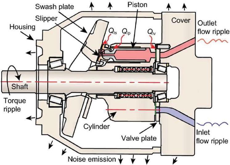
Figure 1 Swashplate type axial piston pump [16].
Table 1 Summary of specifications for the Parker P1 pump
| Max. Displacement | 18cc |
| Pressure Range | 0 to 350 bar |
| Speed Range | 600 to 3600 rpm |
| Temperature Range | 40 to 95C |
| Rated Fluid Viscosity | 6 to 160 cSt |
| Pistons | 9 |
| Overcenter Capable | Yes |
| Closed-Circuit | Yes |
It is well known that the main sources of energy dissipation in swashplate type axial piston pumps occur at the slipper/swashplate, piston/cylinder, and valve plate/cylinder block interfaces [17–19]. These three main lubricating interfaces are highlighted in Figure 2. These interfaces are also the locations that exhibit the most wear on a pump, not including the roller bearings [1, 9, 14, 20–25].
The valve plate is a critical component that can experience large amounts of wear and damage. Valve plates contribute to up to 38% of pump failures in some aerospace pumps [9]. For these reasons, the valve plate is the component that is chosen to investigate condition monitoring of axial piston pumps in this work.
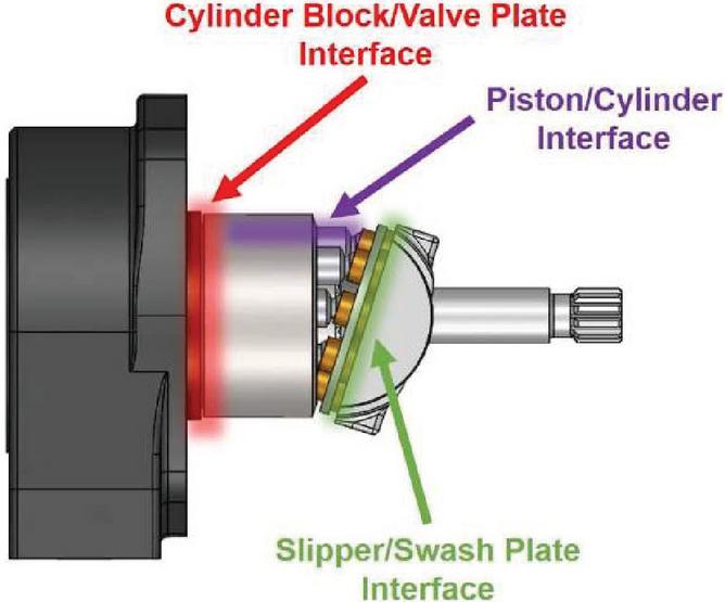
Figure 2 Three main lubricating interfaces of a swashplate type axial piston pump.
2.1.1 Selected valve plates
As mentioned in the introduction, one of the challenges of this method is possessing multiples of a component each with varying levels of damage or wear. In this work, five valve plates with varying degrees of wear and damage are used to perform the necessary experiments. It must be noted that real production units might have higher variations in the results. It is recommended to employ a statistical analysis involving a larger population of “healthy” and faulty units. In this work, wear is the result of metal-to-metal contact between the valve plate and the cylinder block, and damage is the result of cavitation or foreign particles causing damage to the valve plate. It is important to note that the effects on the performance of the pump with the various states of valve plate health cannot be exactly known and is difficult to predict because of the high nonlinearity of these interfaces [23]. The selected valve plates can be seen in the list below.
1. No Wear with No Damage (Healthy)
2. Severe Wear with No Damage (SW_ND)
3. Minor Wear with Moderate Damage (MinW_ModD)
4. Minor Wear with Severe Damage (MinW_SD)
5. Moderate Wear with Minor Damage (ModW_MinD)
Each of the different degrees of wear on the valve plates occurred naturally while the pump was mounted on a mini-excavator. Four valve plates with varying degrees of wear have been obtained: no wear, minor wear, moderate wear, and severe wear. The wear profile on each of the valve plates is measured using a ZeGage optical profilometer. The wear profile is measured at the same location for each of the valve plates for consistency. Manufacturing tolerances have not been taken into account and are considered negligible in this work.
The valve plate that appears to have negligible wear is considered the healthy valve plate. The profilometer measurements of the healthy valve plate can be seen in Figure 3 and show sub-micron variation of surface wear. Therefore, this valve plate is considered to have negligible wear and no damage. The lower left black plot in Figure 3 is the zoomed green profile that can be seen in the upper left surface image of the valve plate in Figure 3.
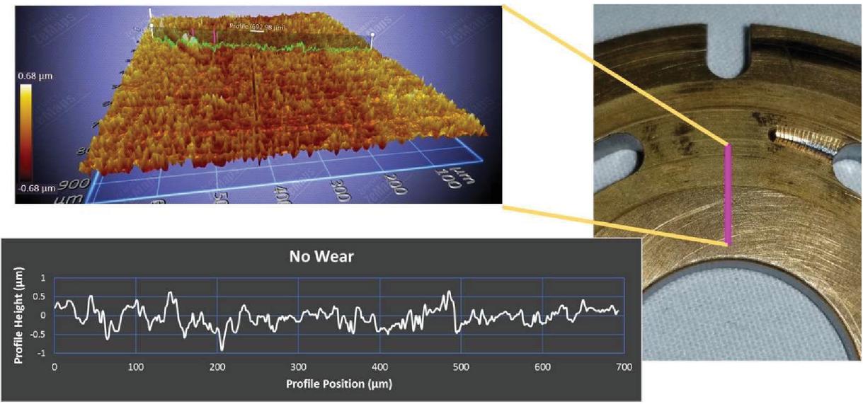
Figure 3 Valve plate with negligible wear and damage.
The wear profiles of the remaining valve plates have more drastic results. The valve plate that exhibits minor wear is measured and shown to have approximately a four-micrometer wear profile, see Figure 4. Figure 5 shows the profilometer measurements of a valve plate with moderate wear, where a wear profile of about ten-micrometers can be observed. The final wear classification for the valve plates is the severe wear case, Figure 6. Not only is the wear profile of the severely worn valve plate 20 micrometers, but a ridge at the edge of the wear interface with a height of 20 micrometers is present. It is speculated that this ridge is caused by the contact of the cylinder block and valve plate. The cylinder block acts as a plow deforming the soft alloy material of the valve plate.
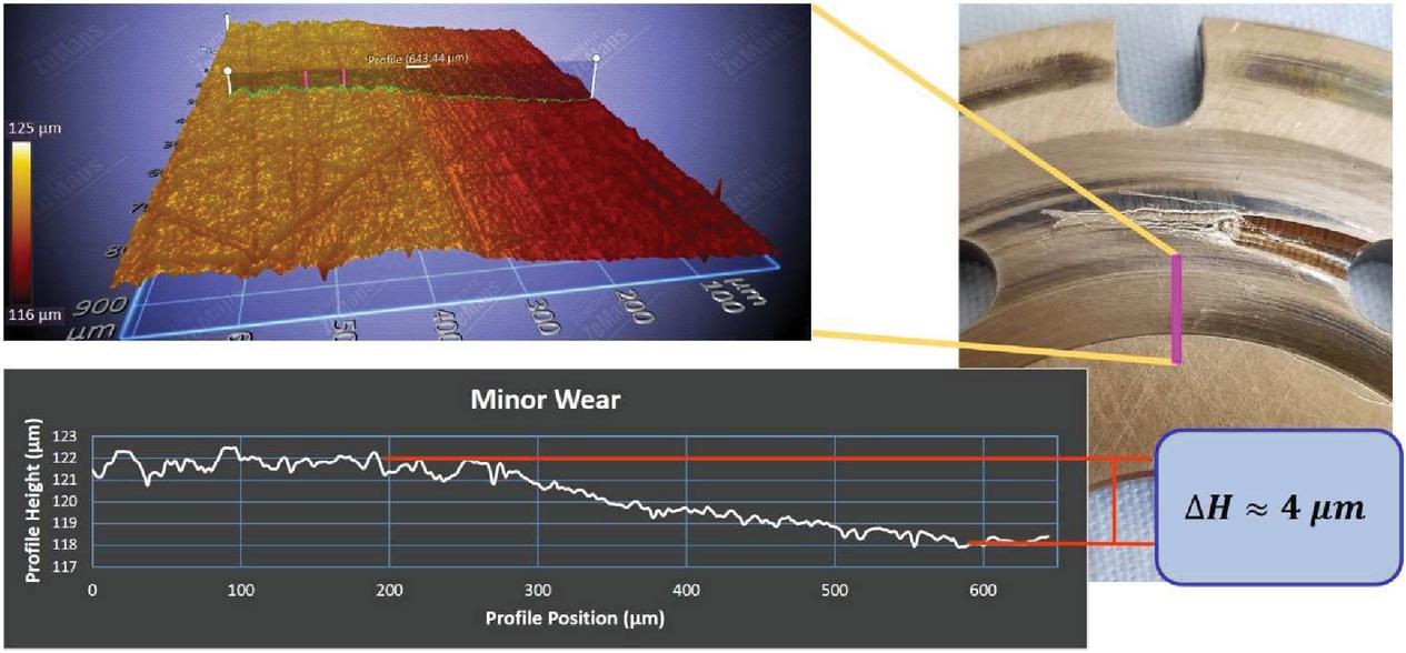
Figure 4 Valve plate with minor wear.
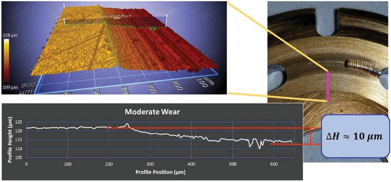
Figure 5 Valve plate with moderate wear.
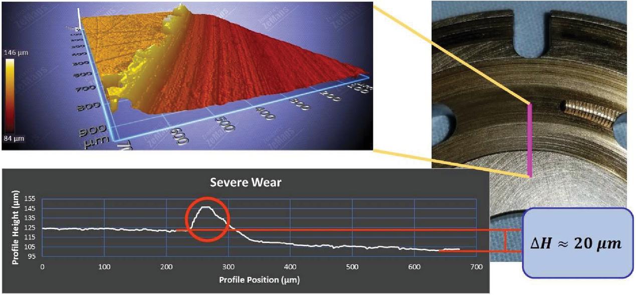
Figure 6 Valve plate with severe wear.
2.1.2 Valve plate damage
To observe the effects that a damaged valve plate would have on the performance of the pump, some valve plates have been artificially damaged at the relief groove on the suction side of the valve plate. The artificially induced damage is intended to simulate damage from debris particles gouging and removing material at the suction side of the pump. This debris could have come from another segment in the system or have been caused by cavitation. It is to be noted that these valve plates are not used to classify what type of damage has occurred. Rather, the purpose is to determine whether general valve plate damage is detectable.
The damage was caused by using a tungsten carbide tip scriber to manually scratch the surface of the valve plate. The scratches were placed in approximately the same location with varying degrees of depth. An optical profilometer is used to observe the profile of the damage. Four levels of damage are performed and measured: No damage, minor damage, moderate damage, and severe damage.
Figure 7 shows the minor damage that is induced on the suction relief groove on the valve plate. The scratch was placed in a radial pattern as to follow the motion of the cylinder block relative to the valve plate. The damage has a depth of approximately 30 micrometers but is less than 0.5 micrometers in width.
The valve plate with moderate damage, Figure 8, has several scratches approximately 15 micrometers deep and span about 25 microns. The damage to the relief groove on the next valve plate is severe, Figure 9, and shows the depth of the damage to vary between 20 and 80 micrometers and spans over 800 micrometers. Not measured but shown is a major dent that has been induced on the relief groove of the valve plate. This damage is induced to provide a severe case to simulate severe abrasion or cavitation damage.
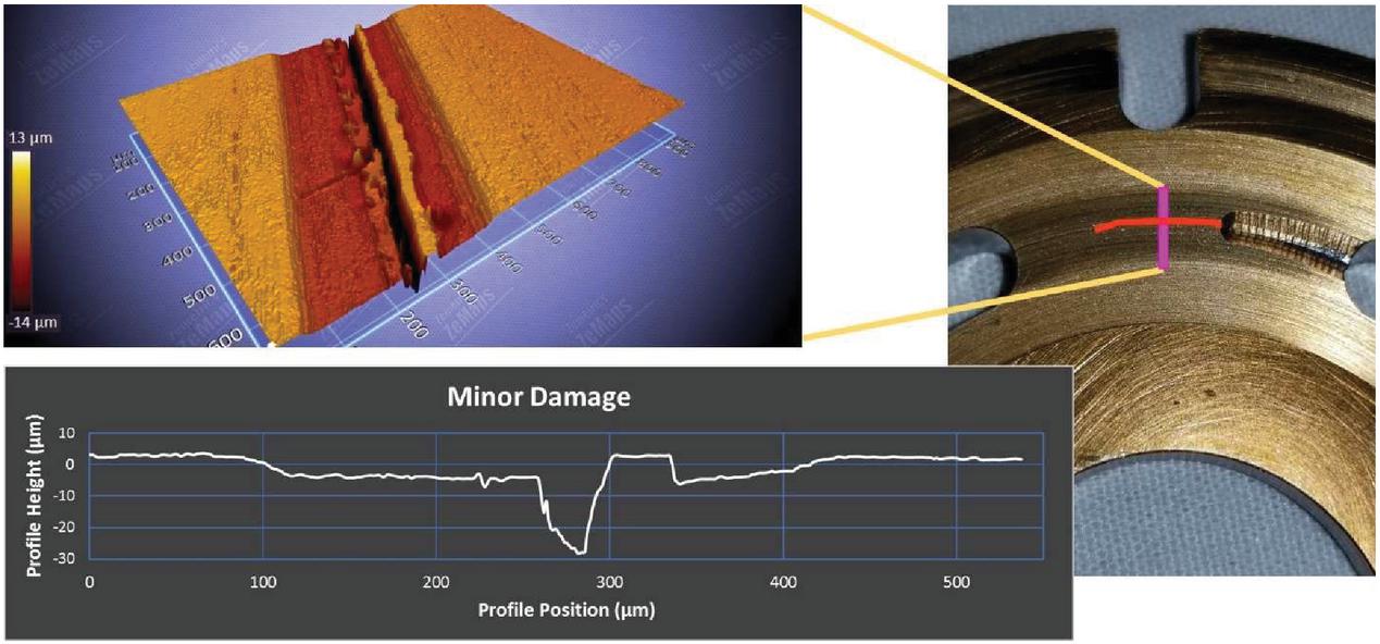
Figure 7 Valve plate with minor damage.
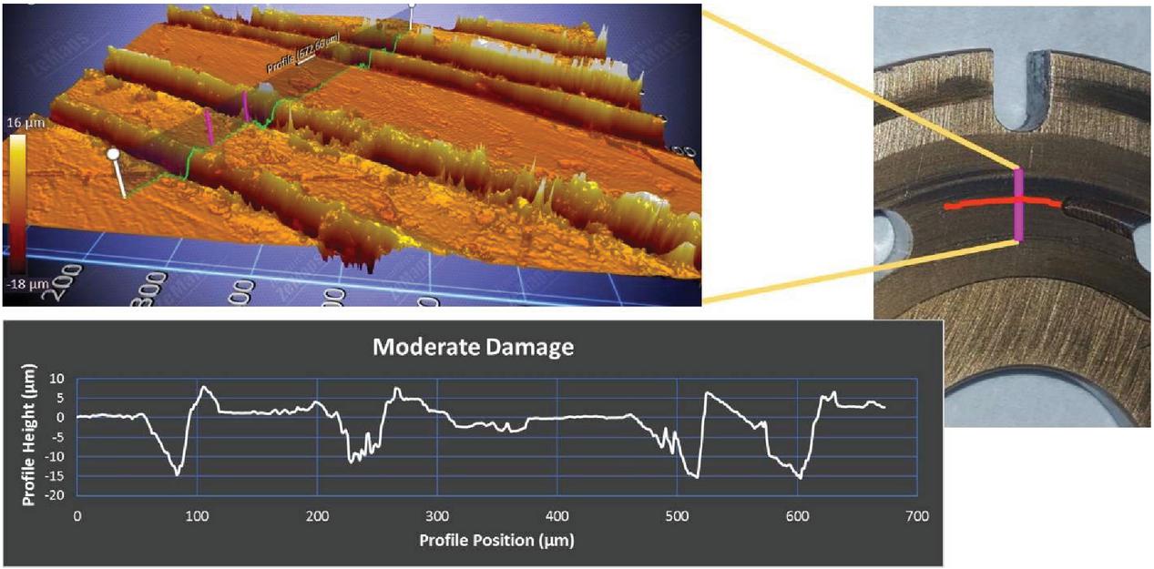
Figure 8 Valve plate with moderate damage.
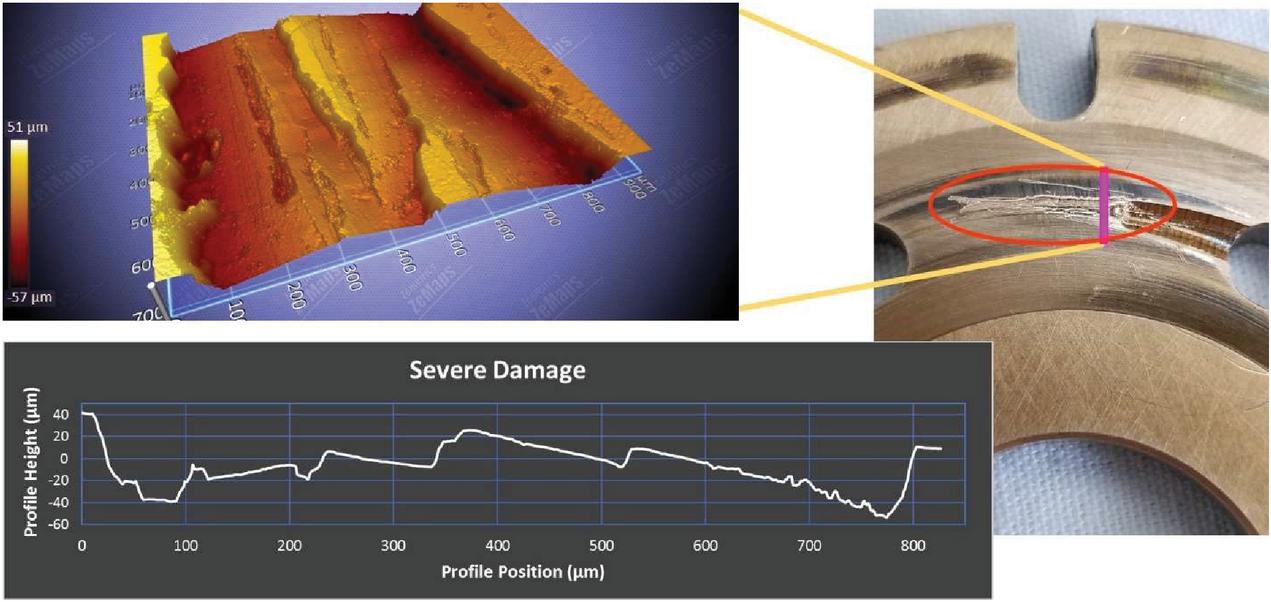
Figure 9 Valve plate with severe damage.
2.2 Stationary Test-Rig
A test-rig is necessary for demonstrating a condition monitoring process for axial piston pumps. Three main purposes exist for the stationary test-rig: perform fault detectability, sensor/dimensionality reduction, and machine learning algorithm selection. The stationary test-rig can be seen in Figure 10 with a few of the highlighted sensors used in the experimental setup. The nomenclature of these captions can be found in Figure 11.
This section will introduce the experimental setup, hydraulic schematic, and the duty cycles used in the measurement process of the test-rig.

Figure 10 Stationary test-rig.
2.2.1 Hydraulic schematic
The description of the hydraulic schematic begins with the Parker P1 pump. The 18cc pump (1) is driven by an electric motor (2), see Figure 11, and receives hydraulic fluid at 25 bar from a constant pressure source provided by power supply located at Purdue University. The pump sends the flow through a gear-type flow meter (7) and, either, over a pressure relief valve (3) or through a variable orifice (4). Two gear-type flow meters measure the drain flow (8) and control flow (9), respectively.
Pressures are monitored and measured at the outlet (16 and 17), supply (13), control (14), and drain (15) lines. All the pressure sensors are piezoresistive, except for the additional piezoelectric pressure sensor on the pump outlet (16), which is capable of measuring the pump’s pressure ripple.
The pump supply (10), outlet (11), and drain (12) temperatures are monitored with a thermocouple. An additional thermocouple, not shown in Figure 11, is mounted outside the hydraulic test-rig near the pump to capture the ambient air temperature.
The shaft torque (5) and speed (6) are measured with a torque meter that contains an integrated speed sensor. The pump displacement is measured using a Hall effect sensor (18) that senses the relative position of the swashplate. Finally, nine single axis accelerometers (19) are mounted on the pump in various locations.
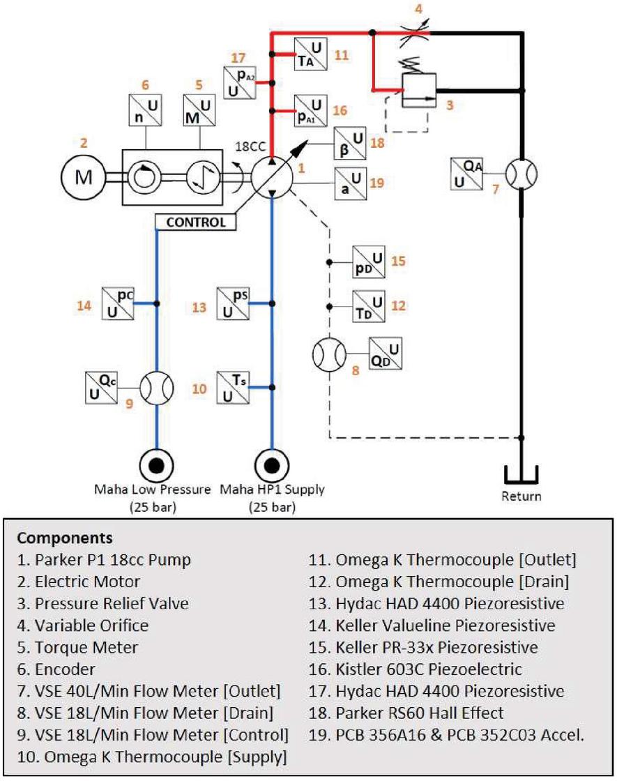
Figure 11 Test-rig hydraulic schematic.
2.2.2 Accelerometer placement
Nine single axis accelerometers are mounted on the outside casing of the pump to measure the vibrations throughout the pump, see the accelerometer mounting locations in Figure 12. Critical locations, such as at the pump inlet, outlet and roller bearings are selected because of the presence of higher vibrations based on previous experience and literature review. However, other locations are considered to ensure adequate coverage of the pump. The purpose of so many accelerometers is to determine the location that has the highest vibrational magnitudes, and to use that location for condition monitoring purposes.
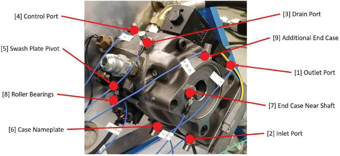
Figure 12 Placement of accelerometers on reference pump.
2.2.3 Duty cycles
The duty cycles are split into two main groups: steady-state and dynamic. The steady-state duty cycle aids in the observations of the data and fault detectability. The dynamic duty cycle simulates the dynamic and transient conditions that could be seen on a mobile machine but in a controlled environment.
Three steady-state operating conditions are utilized in this work, see Table 2. The procedure strictly respected the condition of reaching steady-state conditions in terms of shaft speed, operating pressures and temperatures, including drain temperatures. This means that the measurements were recorded with negligible drift over time.
Table 2 Steady-state operating conditions
| Operating | N | p | ||
| Condition | [RPM] | [] | [C] | [bar] |
| OpCon_1 | 100 | |||
| OpCon_2 | 2000 | 1 | 52 | 150 |
| OpCon_3 | 200 |
The purpose of the dynamic cycle is to determine if the faulty components are detectable under transient operating conditions. A simple and repeatable method to produce a dynamic cycle is through the use of an orifice while varying the displacement of the pump under a constant speed condition. The pressure, or load condition, follows the orifice equation seen in Equation (1).
| (1) |
The dynamic duty cycle is achieved by setting the relief valve to a setting of 200 bar and restricting the variable orifice to a setting that allows all the flow from the pump with a 50% displacement to pass through the orifice with a pressure drop of about 25 bar. The orifice area is then kept constant, and the pump displacement is varied from about 0.5 to 1.0 of the normalized swashplate position. Figure 13 is an example of how the pressures change dynamically as the pump displacement it varied.
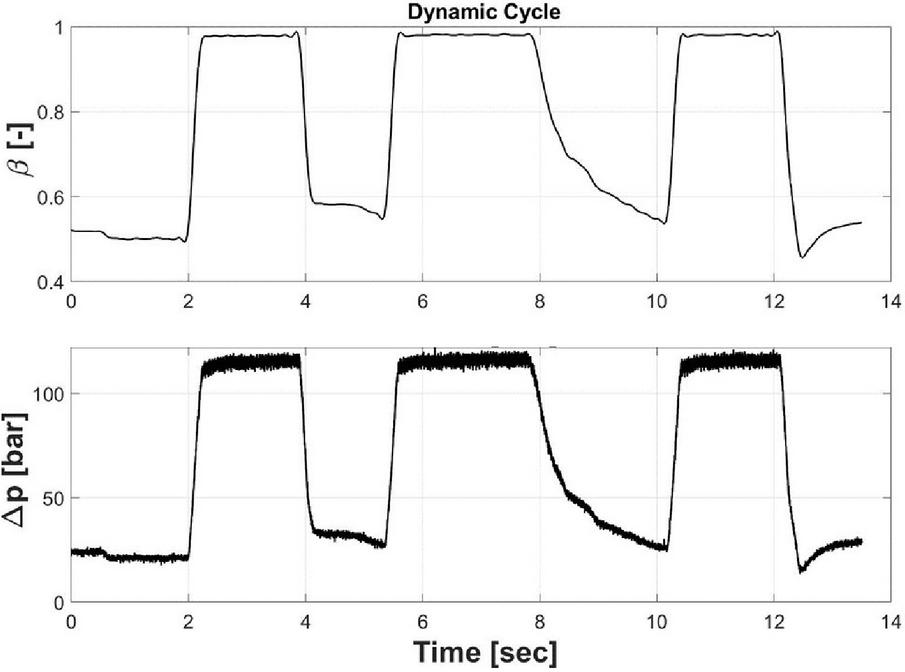
Figure 13 Dynamic duty cycle.
3 Analysis
The analysis portion of this work includes the measurement observations made by a human, the feature selection/sensor reduction methodology, the algorithm selection methodology, and their corresponding results.
The sensor reduction as well as the selection of the best algorithm for the reference part are critical steps that should not be overlooked. As mentioned in the introduction, this sensor selection improves the CM model’s overall performance by avoiding result overfitting, lowers the total cost of the CM device, and expands its applicability to mobile machines. The output of each CM algorithm varies depending on the application and the sensors used. As a result, in order to ensure the best performance of the CM method, a thorough examination of the various algorithms is required.
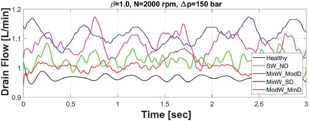
Figure 14 Drain flow of healthy and unhealthy valve plates.
3.1 Measurement Observations
It is valuable for a human to observe if differences in pump behavior exist between the various states of pump health, regardless of an AI program. Human judgement is also a necessity to ensure the machine learning algorithm is fed the correct data.
Increased drain flow is a logical result of a damaged valve plate due to the increase in leakage. The comparison of drain flow between the healthy and unhealthy conditions can be seen in Figure 14. Each of the unhealthy valve plates produces more drain flow (leakage) than the healthy valve plate. This one confirmation shows that a difference is observed between the healthy and unhealthy valve plates.
3.2 Feature Selection/Sensor Reduction
With observable differences between the healthy and unhealthy machines confirmed, it is now time to begin investigating the machine learning aspect of this work by starting with the feature selection process. Feature selection is the process of reducing the number of features or dimensions in the data that will be fed into the machine learning algorithm. Reducing the number of features can, in turn, reduce the number of sensors required for monitoring the condition of a pump. Consequently, this reduction makes the CM system less expensive and easier to incorporate in mobile applications.
A brief background on feature selection will be discussed. Next, the different accelerometers are compared to look for redundancy. Finally, a backward elimination feature selection is shown to reduce the number of sensors required to accurately detect the healthy and unhealthy pumps.
3.2.1 Feature selection background
The complexity of machine learning algorithms determines the number of input dimensions, or features, and the sample size, which determines computational cost and memory usage [26]. Dimensionality reduction not only reduces the computational cost and memory usage, but it also generates simpler models that are robust and more protected against overfitting [26–28].
Dimensionality reduction can be summarized into two main categories: Feature extraction, and feature selection [26–28]. Feature extraction focuses on generating a new set of features by combining features from the original dataset, i.e. Principal Component Analysis (PCA). Feature selection generates a new subset by selecting a certain number of features from the original dataset without combining features. The goal is to select the relevant features and generate a small subset to reduce the complexity of the data. Irrelevant or redundant features add little to no benefit to the performance of the machine learning algorithm [29]. Eliminating irrelevant or redundant features can mean a reduction in sensors required in the experimental measurements. The method of feature selection used in this work backward elimination.
Backward elimination starts with the maximum number of features and eliminates one feature at a time until a simplified subset is generated that results in high accuracy and algorithm performance. The backward elimination method is selected for the work because of its robustness against overfitting, ease of use, and wide acceptability [28]. Many other feature selection methods exist that vary in complexity and reliability [26, 27, 29, 30].
3.2.2 Accelerometer location comparison
Nine accelerometers are mounted on the case of the pump and an analysis must be conducted to reduce the required number of sensors. Previous work has shown that only the amplitudes of the accelerations differ from one accelerometer location to another without a difference in the frequencies of the signals [13, 31]. If the accelerometer location only affects the magnitude and not the frequency content of the signals, then it is possible to only have a single accelerometer for condition monitoring purposes.
This work confirms previously performed research that only the magnitude and not the frequency content of the accelerations changes with the location of the accelerometer, for comparison purposes. For brevity and illustrative purposes, the frequency domain of only four accelerometers at different locations are compared by taking the Fast Fourier Transform (FFT) of the vibration signals, see Figure 15. Zooming in, Figure 15(c), it is clear that only the magnitude of the signals varies and not the frequency. For this work, the accelerometer located on the case near the roller bearings produced the higher magnitude of vibrations. This means a single accelerometer will be used in this investigation into which sensors are most beneficial in the condition monitoring process.

Figure 15 Comparison of accelerometers at the locations of the drain port, roller bearing, end case, and the swash plate pivot.
3.2.3 Backward elimination method and result
Several criteria are used to methodically eliminate certain features/sensors. First, an accelerometer comparison was made and was determined that a single accelerometer is sufficient to detect changes in the vibrational characteristics of the pump. Next, the cost and robustness of the sensor is considered. Torque sensors and flow meters are expensive, prone to damage, and have larger geometric footprints. Cost, reliability, and size of these sensors make them less than ideal for mobile hydraulic applications. Finally, the performance of the machine learning model is observed. This includes the model training time, prediction speed, accuracy.
This paper utilizes existing tools and algorithms to demonstrate a condition monitoring process and does not develop and introduce new algorithms. The Classification Learner App in MATLAB is used to perform the feature selection, which will help determine the most important and relevant sensors for the condition monitoring algorithm. The Fine Decision Tree is used during each iteration of the backward elimination process to observe how different features influence the accuracy of the model. Later, additional algorithms will be considered with the reduced features. The accuracy is calculated based on the ratio of the number of correctly classified data points to the total number of data points entered into the classification algorithm.
Table 4 shows a summary of the results from the feature selection for each of the operating conditions, while Table 3 shows feature abbreviations. A full example of OpCon_1 can be seen in Table 7 in Appendix A. However, the summary in Table 4 gives valuable information as to which sensors seem to provide the best accuracy to the machine learning model.
For the steady-state operating conditions, two sets of features produce the best results. The drain pressure (pD), drain flow (QD), and pump displacement (Beta) produce the model with the highest accuracy of 99.1% to 100%, depending on the operating condition. However, the outlet pressure (pA2), inlet pressure (pS), drain pressure (pD), and pump displacement (Beta) give the second-best results for the steady-state operating conditions with accuracies from 98.6% to 99.6%. This second set of features does not contain a flow meter, which would greatly reduce the cost and complexity of instrumentation with only a minor reduction prediction accuracy.
Table 3 List of features with their corresponding abbreviations
| Abbreviations | Description |
| pA2 | Outlet Pressure |
| pS | Supply or Inlet Pressure |
| pD | Drain Pressure |
| QD | Drain Flow |
| Beta | Pump Displacement |
| N | Pump Rotational Speed |
Table 4 Feature selection summary
| Features/Sensors | Accuracy [%] | |
| OpCon_1 | pA2, pS, pD, Beta | 99.6 |
| pA2, pD, Beta | 99.5 | |
| pD, QD, Beta | 100 | |
| pD, Beta | 99.2 | |
| QD, Beta | 99.5 | |
| OpCon_2 | pA2, pS, pD, Beta | 99.2 |
| pA2, pD, Beta | 98.8 | |
| pD, Beta | 98.8 | |
| pD, QD, Beta | 99.1 | |
| QD, Beta | 97 | |
| OpCon_3 | pA2, pS, pD, Beta | 98.6 |
| pA2, pD, Beta | 98.2 | |
| pD, Beta | 97.9 | |
| pD, QD, Beta | 99.7 | |
| pD, QD | 97.7 | |
| QD, Beta | 99.4 | |
| Dynamic | pA2, pD, Beta, N | 86.4 |
| pA2, pS, pD, Beta, N | 88.5 | |
| pA2, pD, N | 84.3 | |
| pA2,pS, pD, Beta | 83.6 | |
| pD, N | 83.9 |
The dynamic operating condition has a lower accuracy, which is to be expected. The feature set that gives the best accuracy of 88.5% for the dynamic duty cycle consists of outlet pressure (pA2), drain pressure (pD), pump displacement (Beta), and pump speed (N). The runner-up is the feature set that gives an accuracy of 86.4% and consists of outlet pressure, inlet pressure, drain pressure, pump displacement, and pump speed.
In summary, the inclusion of a flow meter mounted in the drain line gives the best accuracies for determining the health of the axial piston pump with regards to the valve plate. This also results in the lowest number of sensors to receive the highest accuracy. However, flow meters are extremely costly and sensitive to contamination, so sacrificing a small amount of accuracy for more sensors at lower cost is a viable option.
Results Summary
In summary, a feature selection process was shown to reduce the number of required sensors to accurately and effectively detect a faulty valve plate on an axial piston pump. First, the number of accelerometers was reduced from nine to one using methods originally proposed by [31]. Next, the number of sensors was further reduced by implementing the backward elimination method. The number of sensors was reduced from 23 to a few combinations containing three to five sensors.
3.3 Condition Monitoring Algorithm Selection
A condition monitoring system requires the best combination of sensors and machine learning algorithms to provide an accurate determination of the condition of the pump. The number of sensors required to accurately classify a healthy and unhealthy pump has been narrowed down to a few different combinations of sensors. With this reduced number of sensor combinations the algorithm selection process will require fewer iterations to find a suitable algorithm and sensor combination. This section discusses what software is used to perform the algorithm selection, as well as a brief background on a K-Nearest Neighbor and decision tree algorithms. Finally, the algorithm selection results will be presented.
Only the classification algorithms that showed the best results will be discussed in this work for brevity. The algorithms have been implemented using MATLAB’s machine learning toolboxes and have not been developed by the author of this work. These algorithms are K-Nearest Neighbor (KNN) and decision trees.
Brief Background on K-Nearest Neighbor (KNN)
K-Nearest Neighbor (KNN) is non-parametric and one of the best-known classification and regression machine learning algorithms [32, 33]. The basic principle of KNN is that it assigns an unclassified data point to the classification of the nearest set of previously classified points. In other words, the unclassified data point takes on the classification of its “nearest neighbor.” As this is a well-known classification method, it is not to be discussed in this work.
MATLAB’s classification learner contains several different KNN classification algorithms and many have been used in the investigation. Four different KNN algorithms have been investigated: Fine, medium, coarse, and weighted. Essentially, the difference between each of the KNN algorithms is how many neighbors the data point is compared to, the k value. Weighted KNN is a variation of KNN where the closer classified datapoints are given higher weights than those farther away from the unclassified datapoint [34].
Brief Background on Decision Trees
Decision trees are another common type of classification algorithm that can be used for nonlinear mappings of input variables to a set of output variables. Decision trees break up the complex decision-making process into several simpler and smaller decisions. Trees are easy to interpret, provide needed insight into the data, and often produce models that have high prediction speeds [27]. Detailed explanations of decision trees can be found in literature [26, 27].
MATLAB contains three different decision tree algorithms in the Classification Learner toolbox: Fine, medium, and coarse decision trees. Decision trees in MATLAB’s classification learner are categorized by the maximum number of splits, or branches, the algorithm is allowed to contain. The more branches or splits a tree contains then the finer the tree becomes.
Algorithm Selection: Steady-State Results
The four sets of features/sensors previously discussed have been selected to compare the different classification algorithms using MATLAB’s Classification Learner Application. Table 5 shows the results for OpCon_2, and how the machine learning model accuracy and performance are influenced by the different algorithms. Only the results from OpCon_2 are shown because the two other steady-state operating conditions give near identical results with the same conclusion.
Table 5 is divided into four separate tables, where each table represents a single combination of features that are applied to several different algorithms. For example, Table 5(a) uses pump outlet pressure, inlet pressure, drain pressure, and pump displacement as fixed features while varying machine learning algorithms to determine the “best” performer, which is the Fine KNN algorithm. This provides the best accuracy of 99.9% with a good prediction speed of 650,000 observations per second, and a low training time of only 23.5 seconds.
Table 5 Algorithm selection results for OpCon_2
|
|
||||||||||||||||||||||||||||||||||||||||||||||||||||||||||||||||||||||||||||||||||||||||||||||||||||||||||||||||
| (a) | (b) | ||||||||||||||||||||||||||||||||||||||||||||||||||||||||||||||||||||||||||||||||||||||||||||||||||||||||||||||||
|
|
||||||||||||||||||||||||||||||||||||||||||||||||||||||||||||||||||||||||||||||||||||||||||||||||||||||||||||||||
| (c) | (d) |
Table 5(b) shows that the Weighted KNN algorithm has the highest accuracy of 99.5%, but has a considerably slower prediction speed than the Fine KNN. The Fine KNN has a negligibly lower accuracy of 99.4%. This means the Fine KNN will have a lower computational cost and is a more efficient algorithm without losing accuracy.
Table 5(c) and 5(d) use the “best” features for the dynamic duty cycle and also show that the superior algorithm is the Fine KNN, which exhibit high accuracies and high prediction speeds, thus lower computational expenses are required.
Observing each condition in Table 5, it can be seen that the decision tree algorithms have exceptionally fast prediction speeds but sacrifice accuracy. It is interesting to note that each of the four-feature combinations give nearly identical results, thus verifying that either of the four feature sets are reasonable to select for the selected condition monitoring purpose.
Algorithm Selection: Dynamic Results
The same process used for algorithm selection for the steady-state conditions is used for the dynamic duty cycle. Table 6 shows the comparison of algorithm performance using the same set of features/sensors that are shown in Table 5. The results for the dynamic cycle are similar to those of the steady-state cycles, and the Fine KNN algorithm gives the highest accuracies with fast prediction speeds and low training times. Another similar result is that each of the four-feature sets have similar performance using the Fine KNN.
Table 6 Algorithm selection results for the dynamic duty cycle
|
|
||||||||||||||||||||||||||||||||||||||||||||||||||||||||||||||||||||||||||||||||||||||||||||||||||||||||||||||||
| (a) | (b) | ||||||||||||||||||||||||||||||||||||||||||||||||||||||||||||||||||||||||||||||||||||||||||||||||||||||||||||||||
|
|
||||||||||||||||||||||||||||||||||||||||||||||||||||||||||||||||||||||||||||||||||||||||||||||||||||||||||||||||
| (c) | (d) |
Results Summary
An algorithm selection process was conducted comparing various versions of KNN and decision tree machine learning algorithms. The Fine KNN machine learning algorithm performs well by producing a model with high accuracy, fast prediction speed, and a low training time. The four-sets of features give similar results, so the selection is up to what is cost effective and easier to implement on mobile equipment. For this study, it seems reasonable to include the pump outlet pressure, inlet pressure, drain pressure, speed, and displacement. Including a flow meter is cost prohibitive for mobile equipment and is sensitive to contamination. Therefore, the final number of sensors is reduced from 23 to 5. The combination of the Fine KNN machine learning algorithms and the five selected sensors is an economical and effective solution for monitoring valve plate faults on axial piston pumps.
4 Conclusion
In the past, failures in fluid power systems have been unexpected and resulted in monetary and productivity losses. However, today’s sensor technology and available computing power enables mobile fluid power systems to be equipped with a condition monitoring system to mitigate failures and machine downtime.
This work provides novel contributions to the field of fluid power and condition monitoring research. Firstly, different valve plates with quantifiable wear and damage were used for condition monitoring on axial piston pumps. Next, a successful investigation was made using existing condition monitoring methods to show it is possible to detect a damaged pump under dynamic operating conditions. Lastly, this work shows a sufficient number of sensors necessary to successfully detect a fault condition of the pump. The FFT analysis determined that the accelerometer placed on the pump case near the roller bearings provides the most significant results. FFT analysis was possible to determine the most significant accelerometer, the one placed on the case near the roller bearings. The other sensors are selected by using the Classification Learner App in MATLAB. From this study, it is possible to determine that the pump outlet pressure, inlet pressure, drain pressure, speed, and displacement are the only necessary parameters to observe for valve plate failure, in conjunction with simple classification machine learning algorithms.
The process of developing a condition monitoring algorithm for axial piston pumps with valve plate wear has been successfully demonstrated with the intent to implement this system on a mobile machine. The procedure demonstrated in this work could be used in industry R&D, but more variables could be introduced to enhance the stochastic significance of the data and more in-depth sensor analysis can be performed. The cost-effective sensor selection used for condition monitoring of an axial piston pump can now be implemented in a mobile condition monitoring process, such as on a mini-excavator.
Appendices
Appendix A: Backward Elimination of OpCon_1
Table 7 Backward elimination results of OpCon_1 using a Fine Decision tree with 25% hold-out validation not using the parallel solver
| Training | Prediciton | Reason | ||||
| Time | Accuracy | Speed | Features | Selected | for | |
| Features | [sec] | [%] | [M obs/sec] | Removed | Features | Removal |
| 17/17 | 101.73 | 100 | 1.7 | Temps not included (not feasible for dynamic cycles) | ||
| 16/17 | 43.3777 | 100 | 1.8 | QD | Sensor cost | |
| 15/17 | 31.03 | 99.9 | 2 | QC | Sensor cost | |
| 14/17 | 29.532 | 99.9 | 2.2 | QA | Sensor cost | |
| 13/17 | 28.212 | 99.7 | 2.1 | M | Sensor cost | |
| 12/17 | 28.622 | 99.7 | 2.1 | pA1 | Sensor cost | |
| 11/17 | 27.623 | 99.7 | 2.1 | FFT_pA1 | Sensor cost | |
| 9/17 | 20.344 | 99.7 | 2.2 | Back_684, Back_680 | Not feasible for dynamic cycles | |
| 7/17 | 17.062 | 99.7 | 2.2 | FFT_684, FFT_680 | Not feasible for dynamic cycles | |
| 6/17 | 17.443 | 99.7 | 2.1 | c_684 | Possibly redundant sensor | |
| 5/17 | 15.156 | 99.6 | 2.2 | N | pA2, pD, pS, Beta, c_680 | |
| 4/17 | 12.366 | 99.6 | 2.2 | c_680 | pA2, pD, pS, Beta | |
| 3/17 | 12.144 | 99.5 | 2.3 | pS | pA2, pD, Beta | |
| 2/17 | 16.327 | 91.7 | 2.2 | pA2, pD | ||
| 2/17 | 10.398 | 99.2 | 2.3 | pD, Beta | ||
| 2/17 | 11.111 | 95.9 | 2.3 | pA2, Beta | ||
| 1/17 | 10.417 | 93.7 | 2.1 | Beta | ||
| 1/17 | 13.058 | 79.3 | 2.2 | pD | ||
| 1/17 | 15.005 | 88.3 | 2.1 | pA2 | ||
| 1/17 | 31.316 | 79.3 | 2.1 | c_680 | ||
| 1/17 | 11.859 | 91.1 | 2.2 | M | ||
| 1/17 | 15.771 | 97.6 | 2 | QD | ||
| 1/17 | 21.712 | 79.5 | 2.1 | QA | ||
| 2/17 | 18.506 | 98.3 | 2.2 | QD, pD | ||
| 3/17 | 19.536 | 100 | 2.1 | pD, QD, Beta | ||
| 2/17 | 16.724 | 99.5 | 2 | QD, Beta |
References
[1] G. Silva, “Wear generation in hydraulic pumps,” SAE Tech. Pap., 1990, doi: 10.4271/901679.
[2] N. Y. Drozdor, “Tribological Problems in Reliability of Machines,” Sov. Eng. J., no. 5, pp. 5–8, 1985.
[3] J. Watton, Modelling, Monitoring and Diagnostic Techniques for Fluid Power Systems. Springer Science & Business Media, 2007.
[4] W. J. Crowther, K. A. Edge, C. R. Burrows, R. M. Atkinson, and D. J. Woollons, “Fault diagnosis of a hydraulic actuator circuit using neural networks - An output vector space classification approach,” Proc. Inst. Mech. Eng. Part I J. Syst. Control Eng., vol. 212, no. 1, pp. 57–68, 1998, doi: 10.1243/0959651981539299.
[5] G. J. Schoenau, J. S. Stecki, and R. T. Burton, “Utilization of artificial neural networks in the control, identification and condition monitoring of hydraulic systems - An overview,” SAE Technical Papers. 2000, doi: 10.4271/2000-01-2591.
[6] F. Lu, R. Burton, and G. Schoenau, “Feasibility study on the use of a neural network to detect and locate excess piston wear in an axial piston pump,” 1994.
[7] F. Lu, T. Burton, and G. Schoenau, “A Neural Network Based Incipient Fault Detection System for an Axial Piston Hydraulic Pump,” 1995.
[8] T. Ramdén, P. Krus, and J. Palmberg, “Condition monitoring of fluid power pumps using vibration measurements and neural networks trained with complex optimisation,” 1995.
[9] J. Du, S. Wang, and H. Zhang, “Layered clustering multi-fault diagnosis for hydraulic piston pump,” Mech. Syst. Signal Process., vol. 36, no. 2, pp. 487–504, 2013, doi: 10.1016/j.ymssp.2012.10.020.
[10] Y. Lan et al., “Fault diagnosis on slipper abrasion of axial piston pump based on Extreme Learning Machine,” Meas. J. Int. Meas. Confed., vol. 124, no. March, pp. 378–385, 2018, doi: 10.1016/j.measurement.2018.03.050.
[11] I. Baus, R. Rahmfeld, A. Schumacher, and H. C. Pedersen, “Systematic methodology for reliability analysis of components in axial piston units,” ASME/BATH 2019 Symposium on Fluid Power and Motion Control, FPMC 2019. 2020, doi: 10.1115/FPMC2019-1620.
[12] T. Ramdén, P. Krus, and J. Palmberg, “Fault diagnosis of complex fluid power systems using neural networks,” 1995.
[13] T. Ramden, “Condition Monitoring and Fault Diagnosis of Fluid Power Systems: Approaches with Neural Networks and Parameter Identification,” Linkoping University, 1998.
[14] Z. Li, “Condition Monitoring of Axial Piston Pump,” no. November, p. 134, 2005.
[15] C. Lu, N. Ma, and Z. Wang, “Fault detection for hydraulic pump based on chaotic parallel RBF network,” Eurasip Journal on Advances in Signal Processing, vol. 2011. 2011, doi: 10.1186/1687-6180-2011-49.
[16] S.-G. Ye and B. Xu, “Noise Reduction of an Axial Piston Pump by Valve Plate Optimization,” Chinese J. Mech. Eng., vol. 31, 2018.
[17] M. Zecchi, “A novel fluid structure interaction and thermal model to predict the cylinder block/valve plate interface performance in swash plate type axial piston machines,” Purdue University, 2013.
[18] D. Mizell, “A Study of the Piston Cylinder Interface of Axial Piston Machines,” Purdue University, 2018.
[19] A. Busquets, “An Investigation of Micro-Surface Shaping on the Piston/Cylinder Interface of Axial Piston Machines,” Theses and Dissertations Available from ProQuest. Purdue University, 2018, [Online]. Available: https://docs.lib.purdue.edu/dissertations/AAI10748597.
[20] A. Yamaguchi and H. Matsuoka, “A mixed lubrication model applicable to bearing/seal parts of hydraulic equipment,” J. Tribol., vol. 114, no. 1, pp. 116–121, 1992.
[21] T. Kazama and A. Yamaguchi, “Application of a Mixed Lubrication Model for Hydrostatic Thrust Bearings of Hydraulic Equipment,” J. Tribol., vol. 115, no. 4, p. 686, 1993.
[22] T. Kazama and A. Yamaguchi, “Experiment on Mixed Lubrication of Hydrostatic Thrust Bearings for Hydraulic Equipment,” J. Tribol., vol. 117, no. 3, p. 399, 1995.
[23] X. Wang, S. Lin, S. Wang, Z. He, and C. Zhang, “Remaining useful life prediction based on the Wiener process for an aviation axial piston pump,” Chinese Journal of Aeronautics, vol. 29, no. 3. pp. 779–788, 2016, doi: 10.1016/j.cja.2015.12.020.
[24] J. Hertz, A. Krogh, R. G. Palmer, and H. Horner, “Introduction to the Theory of Neural Computation,” Phys. Today, vol. 44, no. 12, pp. 70–70, 1991.
[25] S. Fatima, S. G. Dastidar, A. R. Mohanty, and V. N. A. Naikan, “Technique for optimal placement of transducers for fault detection in rotating machines,” Proc. Inst. Mech. Eng. Part O J. Risk Reliab., vol. 227, no. 2, pp. 119–131, 2013.
[26] E. Alpaydin, Introduction to Machine Learning Second Edition, 2nd ed. Massachusetts Institute of Technology, 2010.
[27] A. R. Webb, Statistical Pattern Recognition, 2nd edn. John Wiley & Sons Ltd., 2002.
[28] J. Tang, S. Alelyani, and H. Liu, “Feature selection for classification: A review,” Data Classification: Algorithms and Applications. pp. 37–64, 2014, doi: 10.1201/b17320.
[29] M. Dash and H. Liu, “Feature Selection for classification,” Intell. Data Anal., vol. 1, no. 1–4, pp. 131–156, 1997.
[30] N. Kwak and C.-H. Choi, “Input feature selection for classification problems,” IEEE Trans. Neural Networks, vol. 13, no. 1, pp. 143–159, 2002.
[31] T. Ramden, K. Weddfelt, and J. Palmberg, “Condition monitoring of fluid power pumps by vibration measurement,” in 10th International Conference on Fluid Power-the Future for Hydraulics, 1993, pp. 263–276.
[32] N. S. Altman, “An introduction to kernel and nearest-neighbor nonparametric regression,” American Statistician, vol. 46, no. 3. pp. 175–185, 1992, doi: 10.1080/00031305.1992.10475879.
[33] A. K. Jain, “Data clustering: 50 years beyond K-means,” Pattern Recognition Letters, vol. 31, no. 8. pp. 651–666, 2010, doi: 10.1016/j.patrec.2009.09.011.
[34] T. Software, “k-Nearest Neighbors.” 2019.
Biographies

Nathan Keller earned his Ph.D. and MS from Purdue University in 2020 at the Maha Fluid Power Research Center. Dr. Keller’s doctoral dissertation focused on demonstrating condition monitoring systems for axial piston pumps for mobile applications. His master’s thesis focused on developing energy saving hydraulic system architectures for the next generation of combine harvesters utilizing Displacement Control (DC) actuation. Dr. Keller has been instrumental in efficient next generation hydraulic designs for agricultural and construction equipment. He was also involved in the realization of the world’s first hydraulic hybrid SUV developed at the Maha Fluid Power Research Center. Dr. Keller is currently employed at Applied Fluid Power as a Systems Product Manager where he assists customers in designing efficient and effective hydraulic system solutions for both industrial and mobile applications.

Annalisa Sciancalepore has been a Ph.D. student in Agricultural and Biological Engineering at Purdue University, IN, the US, since 2018. She received her B.Sc. in Mechanical engineering in 2015 and her M.Sc. in Mechatronic engineer in 2017 from the Polytechnic University of Turin, Italy. Annalisa’s research focuses on hydraulic systems optimization for material-handling machines. Specifically, she is investigating novel hydraulic circuits that use counterbalance valves with an adjustable pilot for energy-saving applications. Moreover, by combining her knowledge of hydraulic with her mechatronic background, she is developing novel numerical and experimental methods for condition monitoring of hydraulic systems and components.

Andrea Vacca holds the Maha Fluid Power faculty chair position at Purdue University, and leads the Maha Fluid Power Research Center of the same University. Dr. Vacca earned his Ph.D. from the University of Florence (Italy) in 2005. Before joining Purdue University in 2010, Dr. Vacca was Assistant Professor of Fluid Machinery at the University of Parma (Italy). Fluid power technology has been Dr. Vacca’s major research interest since 2002. His research team has developed original numerical and experimental techniques for hydraulic systems and components. The team as also formulated several novel solutions, including new concepts to perform hydraulic actuations as well as new designs for pumps and motors. Dr. Vacca is the author of more than 150 papers, most of them published in international journals or conferences. Dr. Vacca is also recipient of the 2019 Bramah medal of the Institution of Mechanical Engineers (IMechE). He is the chair of Fluid Power Systems and Technology Division (FPST) of ASME, and a former chair of the SAE Fluid Power division. Dr. Vacca is also Treasurer and Secretary of the Board of the Global Fluid Power Society (GFPS). Furthermore, he is also Editor in Chief of the International Journal of Fluid Power and he is in the Editorial Board of Actuators, the Journal of Dynamics and Vibroacoustics and the Journal of Hydromechatronic.
International Journal of Fluid Power, Vol. 23_2, 205–236.
doi: 10.13052/ijfp1439-9776.2324
© 2022 River Publishers