Neural Network Identification and Direct Adaptive Fuzzy Neural Network (DAFNN) Controller for Unknown Nonlinear Non-affine Pneumatic Servo System

Peyman Mawlani and Mohammadreza Arbabtafti^*

Mechanical Engineering, Shahid Rajaee Teacher Training Univesrity, Tehran, Iran

E-mail: arbabtafti@sru.ac.ir

^*Corresponding Author

Received 26 December 2019; Accepted 19 November 2020; Publication 27 April 2021

Abstract

In this paper, a direct adaptive fuzzy neural network (DAFNN) controller for trajectory tracking control of the non-linear non-affine pneumatic servo system is presented. First, using a neural network identifier, the non-linear dynamics of a real pneumatic servo system is simulated. By comparing the output of the neural network and the output of the experimental setup, it is observed that the non-linear pneumatic actuator system is well-identified using neural networks. By incorporating the Lyapunov stability theorem, the adaptive laws for the parameters of the controller are obtained, parameter boundedness and stability of the closed-loop system are guaranteed. Finally, practical results are successfully implemented for trajectory tracking control of the pneumatic servo system, in which the effect of the simultaneous updating of the antecedent and consequent’s parameters of the fuzzy neural network controller has been investigated. The tracking error $\pm$1.3mm and $\pm$1 mm for proposed updating method compared to $\pm$2.5mm and $\pm$3.5mm, for a case that the weigh parameters are merely adjusted, are obtained. The results indicate the proposed adjustment method improves the performance of the controller in the presence of unknown nonlinearities and dynamics uncertainty.

Keywords: Adaptive control, fuzzy neural network control, trajectory tracking control, non-affine pneumatic servo system, neural network identifier.

1 Introduction

Pneumatic actuators, on account of low cost, cleanliness, easy maintenance and high power-to-weight ratio, exert numerous benefits to the industry. Despite being exploited these advantages, pneumatic actuators due to some drawbacks, for instance, the air compressibility, the presence of nonlinear factors such as friction force in the cylinder and airflow inside the proportional valve, cannot be modelled accurately. Consequently, achieving a precise control for these systems is challenging. Some researcher (Maré et al., 2000), (Ning and Bone, 2005), accordingly, have endeavoured to design accurate physical models for nonlinear pneumatic actuators.

Identification of pneumatic actuator systems (Al-Saloum et al., 2017), (Osman et al., 2012) provides another supplementary method for modelling these systems. Moreover, In the last few decades, having been emerged the cutting-edge artificial intelligence approaches, its applications are spanned to modelling and controlling nonlinear systems and led to the Neural network identifiers (Neji and Beji, 2000), becoming a favoured method for modelling dynamic systems. This technique- based on the input-output mapping- derives the model of systems in the form of the black box. (Carneiro and de Almeida, 2012) have presented a neural network identification to model the pneumatic servo system. Two perceptron multilayer neural networks have been proposed, one for modelling the flow of mass within the valve, and another for friction modelling in the cylinder. Eventually, assessing the obtained model, they indicated that the position error for 95% of the experiment data is between $-$7.6% and 1.9% of the working range, and the velocity error for 95% of the data is between $-$7.5% and 7.5% of the working range.

Despite the accuracy-barricaded nonlinearities in these systems, their unique advantages motivate researchers to improve some satisfactory control theories for pneumatic systems. Many researchers have challenged their ability to deal with the nonlinear pneumatic actuator system by designing controllers such as adaptive control (Zhu and Barth, 2010), sliding mode control (Laghrouche¶ et al., 2006), back-stepping control (Hajji et al., 2019) and observer-based control (S.-Y. Chen and Gong, 2017).

A new structure of back-stepping controller for an electro-pneumatic system has been designed by (Smaoui et al., 2006). The control law has been developed along with a nonlinear friction model, which leads to the controller performing better than classical linear controllers.

In nonlinear pneumatic system examinations, the mathematical model involves unknown nonlinear dynamics; friction’s mismatched uncertainty and, payload variations result in the classic controller being incapable to creating a precise control action to address these drawbacks. Therefore, nonlinear controllers such as sliding mode control (SMC) (Tsai and Huang, 2008) to overcome these uncertainties could be successfully applied.

Liu et al. (2013) have presented an observer-based adaptive sliding mode controller for the pneumatic system with input dead-zone. Observer-based control coped with unmeasurable states and the states of the system are properly estimated, as well as, the input dead-zone parameters have been updated through adaptive law derived from Lyapunov theory.

In the last decades, utilizing artificial intelligence and soft computing has increased in practical applications. Exploiting their well-known ”universal function approximation” property dealing with unknown and non-linear systems uncertainty, Fuzzy Logic Control (FLC) (Q. Gao et al., 2012) and Neural Networks (NN) controllers (Sun et al., 2013) are two common types of soft computing that could widely solve the engineering problems (for instance, modelling and control of non-linear dynamical systems).

An FLC for a pneumatic system with friction model, the model of the unknown system and external disturbance, has been implemented practically by (Lai and Chang, 2017). Two types of the FLC with friction compensator and FLC combined with the PD and PI controller for pneumatic actuator has investigated and their performance compared. The positioning error for the FLC with the friction compensator and the Fuzzy-PD, Fuzzy-PI controller have been obtained 93.3% and 91.1% below 30 nm, respectively.

Kaitwanidvilai and Parnichkun (2005) have proposed a hybrid force controller including adaptive model reference Neuro-Fuzzy and Bang-Bang control for pneumatic servo system force control. By employing the Bang-bang controller the large error between actual output and set-point has been compensated. To update the parameters of the antecedent and consequent part of the Neuro-Fuzzy controller, the authors have benefited from descending gradient technique.

To overcome time-varying nonlinear dynamics and external disturbances of the pneumatic actuator system, (L.-W. Lee and Li, 2016) applied an adaptive Fourier Neural Network sliding mode controller with $H_{\mathrm{\infty }}$ tracking performance (AFNN-SMC+$H_{\mathrm{\infty }}$). For fast convergence of controller parameters, an orthogonal Fourier basis function has been introduced.

An adaptive Recurrent Neural Network (ARNN) controller contributing control of the pneumatic artificial muscle (PAM) manipulator has proposed by (Ahn and Anh, 2009), The controller structure consists of two ARNN. One has been designed to update the PAM manipulator inverse dynamic model, and the other has been used to produce the proper control signal. The provided controller has good properties, such as high learning speed and flexibility in learning.

X. Gao and Feng (2005) have provided an adaptive Fuzzy-PD controller to control the position of the pneumatic servo system with nonlinear properties. To increase the accuracy of the pneumatic servo position control system, a new control algorithm has been used and a friction compensation method have been done by means of a scaling factor $K_{\mathrm{\Delta }e}$ and an adaptive controller parameter $Ma$.

An FLC with velocity feedback (VF), system lag compensator (LC) and friction compensator (FC) for control the position of the pneumatic actuator system has implemented by (Nazari and Surgenor, 2016). The FLC parameters, VF and FC compensators are tuned offline, and the LC compensator parameters are obtained from an online algorithm. In following, the tracking trajectory problem for sinusoidal references has been experimentally investigated, the results demonstrated that errors of 5 mm, 6 mm and 10 mm are obtained for frequencies of 0.1, 0.2 and 0.5 Hz, respectively.

Motivated by above-mentioned studies, in this paper, a direct adaptive Fuzzy Neural Network (DAFNN) control overcoming the uncertain and unknown of nonlinear non-affine pneumatic actuator system is presented. A multilayer feedforward Neural network identification, in which the delays of input and output should be prepared for the NN model, is utilized to establish an accurate model for the pneumatic actuator system. It, accordingly, does not need a mathematical model for the system. A control signal is directly derived through FNN controller, in which the adaption laws to updating the parameters are investigated. To demonstrate the effect of hybrid tuning method of proposed controller’s parameters, the performance of the controller is compared with a controller in which, only the parameters of the consequent part of the controller are updated. This work pursues some contribution which are outlined as below:

• The NN is used to approximate the time series function based on input-output delays of practical pneumatic system. Therefore, the model eradicates the need for a complex mathematical model of friction forces effected by cylinder and flow mass inside the proportional valve.

• In the term of control design, the FNN controller to approximate the control signal needless for prior knowledge of the system is directly employed. Compared to an indirect approach, the singularity and the complexity of computation could be avoided.

• The proposed control approach reduces the cost of a practical system: FNN controller does not need to measure pressure from the sensors. As a result, a more economical practical system can be achievable with fewer sensors.

• For being more flexible, a hybrid updating method is provided so that the parameters of the antecedent and consequent of the FNN system are simultaneously derived.

The paper is organized as follows. In Section 2, a NN is utilized to obtain the black box model of pneumatic actuator system. In Section 3, DAFNN controller is designed and stability analysis is accomplished for close-loop system. The results for experimental and simulation tests are demonstrated in Section 4. Finally, Section 5 concludes the paper.

2 Modelling and System Description

2.1 System Hardware and Software

In Figure 1 a schematic of pneumatic system has been illustrated which specifically includes components (see Figure 2) such as an SMC cylinder (80 mm bore and 125 mm piston stroke), a proportional directional valve (Festo, Mype-5-1/8-HF-010B model), a linear potentiometer (Opkon, LPT model), a pressure regulator and a tank for storing compressed air. Furthermore, control purpose realization necessitates that in each sample time $dt=0.01s$, some signals (e.g. tracking trajectory error) which are considered controller inputs feedback to the PC through PCI1710U A/D card and appropriate command signal (e.g. control signal) send to servo valve through PCI1710U D/A card.

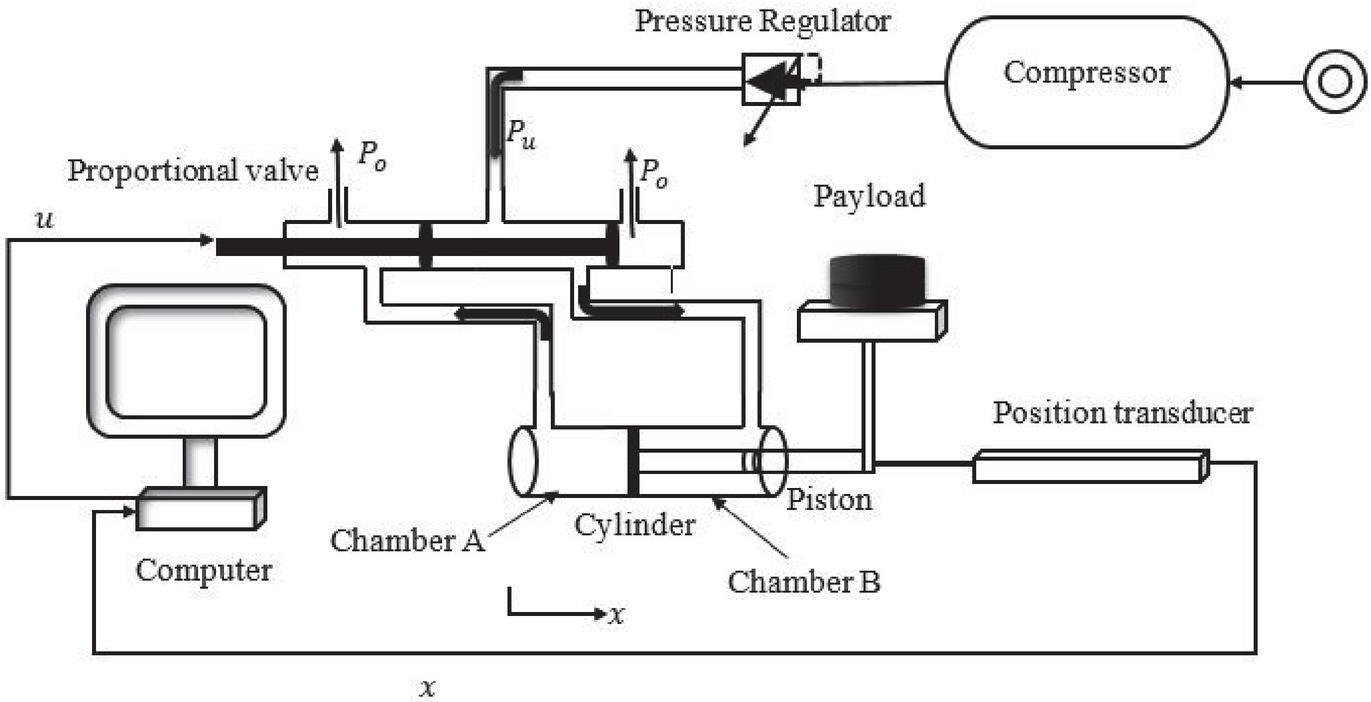
Figure 1 Schematic of pneumatic system.

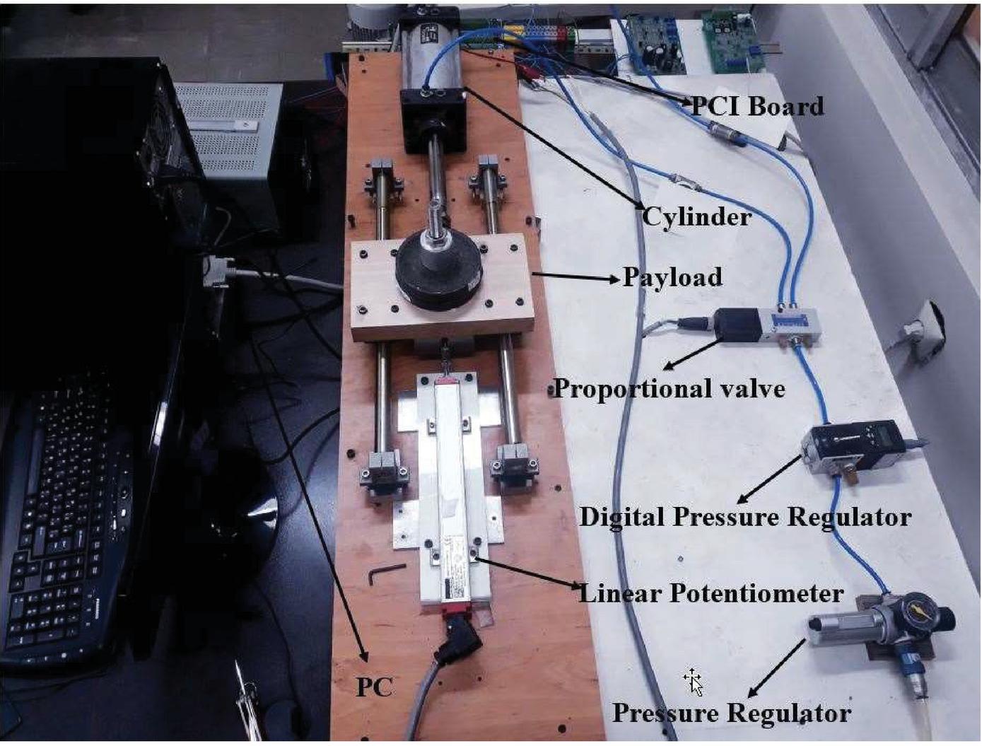
Figure 2 Practical pneumatic actuator system with its components.

2.2 Modelling and Identification

As mentioned, nonlinearities in the mass flow model, friction force in the cylinder, and the dead-zone of the spool valve make pneumatic systems hard to extract an accurate physical model. A summary of principle equations used to model a nonlinear pneumatic actuator has been presented by (Bone and Ning, 2007), which formulated as follows.

${\dot{m}}_a$	$=f_a(P_a,u),{\dot{m}}_b=f_b(P_b,u)$	(1)
$KRT{\dot{m}}_a$	$=K{P}_a{A}_a\dot{x}+A_a(y_{a0}+x){\dot{P}}_a$	(2)
$KRT{\dot{m}}_b$	$=-K{P}_b{A}_b\dot{x}+A_b(y_{b0}-x){\dot{P}}_b$	(3)
$F_p$	$=(P_a{A}_a-P_b{A}_b)$	(4)
$F_l$	$=\{\begin{array}{cc}{F}_p,\hfill & \dot{x}=0and|F_p|\le F_{sf}\hfill \\ F_{sf},\hfill & \dot{x}=0and|F_p|>F_{sf}\hfill \\ F_{cf}+C_{vf}\dot{x},\hfill & \dot{x}>0\hfill \\ -F_{cf}+C_{vf}\dot{x},\hfill & \dot{x}<0\hfill \end{array}$	(5)
$M\ddot{x}$	$=F_P-F_l$	(6)

Where ${\dot{m}}_a,{\dot{m}}_b$ are mass flow with nonlinear relation to pressures $P_a,P_b$ in chamber A and chamber B, respectively and control signal $u$. $K$ is specific heat ratio; $R=287\frac{j}{kg.K}$ is ideal gas constant; $T=293K$ is air temperature. $x$ is piston position with mass $M$ (it includes the masses of payload and piston mass). $A_a,A_b$ are the piston areas of chamber A and chamber B, respectively. $y_{a0}$ is the distance between the piston and the A end of the cylinder when $x=0$; $y_{b0}$ is the distance between the piston and the B end of the cylinder when $x=0$. $F_p$ is the pneumatic force; $F_l$ is the total friction force; $F_{sf}$ the stick-slip friction force; $F_{cf}$ is the Coulomb friction force; $C_{vf}$ is the coefficient of viscous friction.

Ning and Bone (2005) based on step input response and pressure data obtained force friction parameters as, $Fsf=83N$, $Fcf=34N$ and $Cvf=78N/(m/s)$ for the Festo rodless cylinder. Afterwards, they improved the friction model dynamic in (Ning and Bone, 2005) as follows.

$F_l=\{\begin{array}{cc}(F_c+(F_s-F_c)e^{-{(\dot{x}/v_s)}^2})sgn(\dot{x})+F_p\dot{x},\hfill & \dot{x}\ne 0\hfill \\ F_p,\hfill & \dot{x}=0and|F_p|<F_s\hfill \\ F_{s}sgn(F_p),\hfill & \text{otherwise}\hfill \end{array}$

(7)

Where $F_c=1.64N$, $F_s=2.73N$, $F_v=1.22$ N/(m/s) and $v_s=0.04$ m/s.

In this work we replace the system identification method based input-output pairs with physical model of real system. The nonlinear autoregressive exogenous model (NARX) (S. Chen et al., 2007) provides an excellent method for system identification in which the output in time $t$is calculated through input-output pair delays $(u(t-i),y(t-j)i=1,2,\mathrm{\dots },n,j=1,2,\mathrm{\dots },m)$ mapping. To accomplish this measure a feed-forward NN system approximates the nonlinear function of NARX model and a NARX Neural Network (NARXNN) can be made , this choice is reasonable because NNs have some advantages such as having high ability of learning the dynamic of systems.

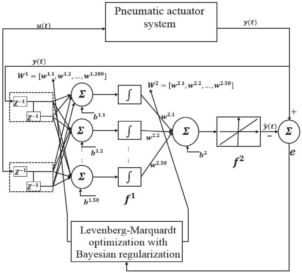
Figure 3 NARXNN diagram for pneumatic system modelling.

The NARXNN diagram for pneumatic system modelling has been shown in Figure 3. As the pneumatic actuator system is considered as second order system, we select two delays of input and output for NARXNN model which is presented as follow.

$$\widehat{y}(t)=FNN(y(t-1),y(t-2),u(t-1),u(t-2))$$

(8)

Where $\widehat{y}(t)$ denotes the NN output.

The precise design requires an appropriate data collection, i.e., frequency-enriched data (the Nyquist frequency law is satisfied) and selected data must cover the workspace of the practical system. In this study, accordingly, to train NN model, we strung all constant input signals together (see Figure 4), and the related output of the pneumatic servo system (position) (see Figure 5) is obtained by applying the designed input.

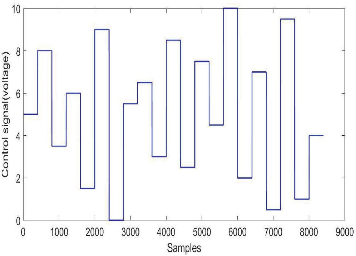
Figure 4 Designed input signal for the proportional valve.

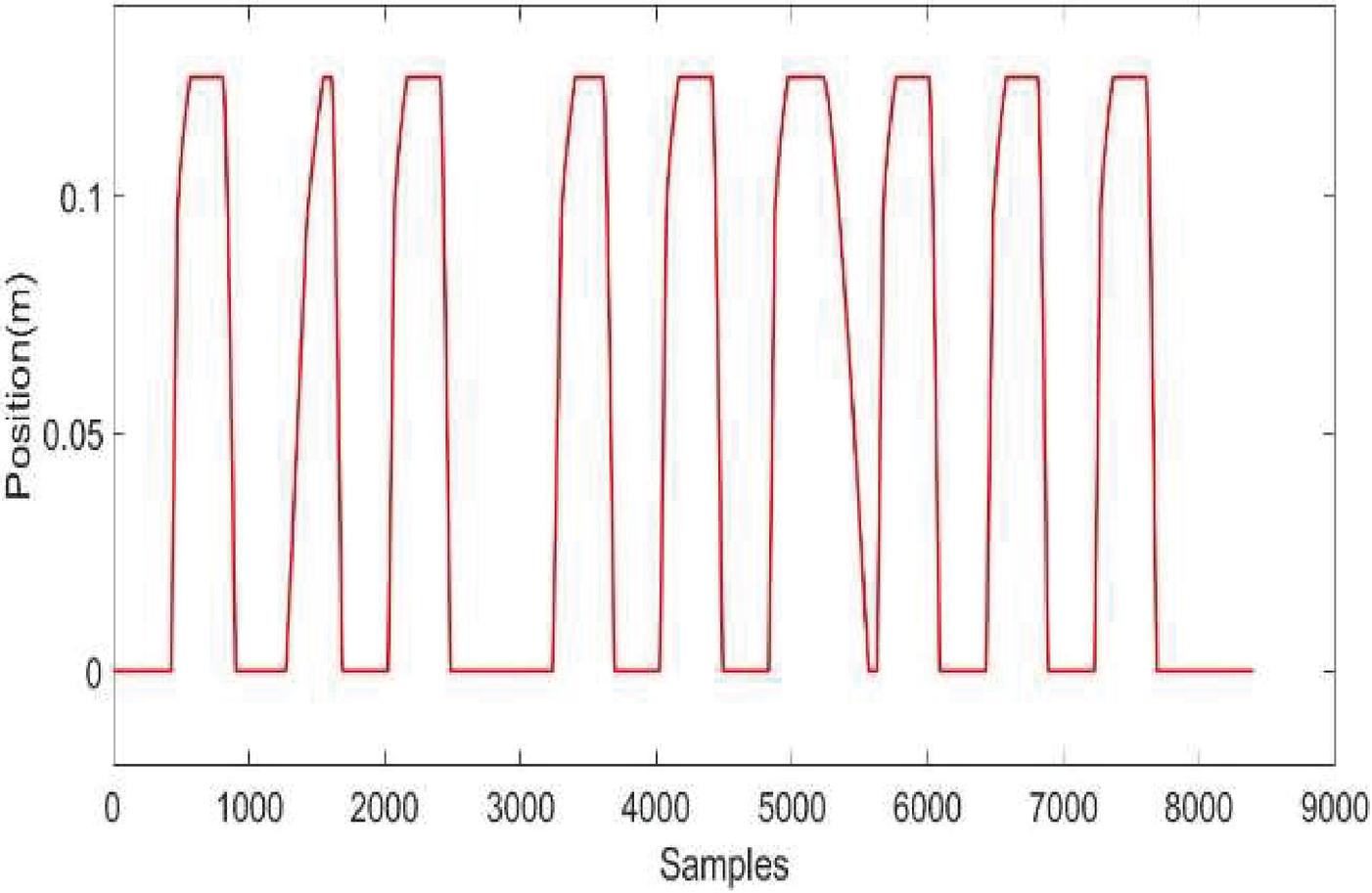
Figure 5 Output signal of pneumatic actuator system.

2.3 Neural Network Model Validation

The neural network (NN) model consists of 50 neurons with Gaussian activation functions in the hidden layer and one neuron with a linear activation function in the output layer. Furthermore, to improve the performance of the model against noisy and complex data, the neural network is trained by the Levenberg-Marquardt optimization algorithm with a Bayesian regularization. The 8400 total data is sampled from which, 5%, 20% and 75% are considered for validation, test and training of NN, respectively. The performance for training and test data is achieved around $3\times {10}^{-7}$ (see Figure 6), indicating that the nonlinear dynamics of the pneumatic actuator system is properly identified.

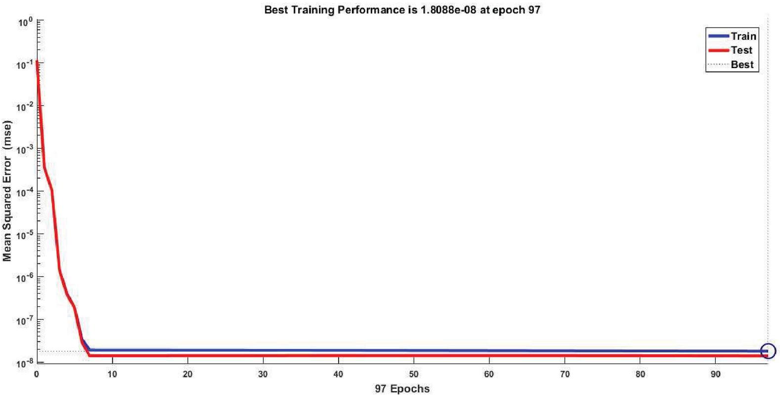
Figure 6 Performance diagrams for training and testing data of neural network model.

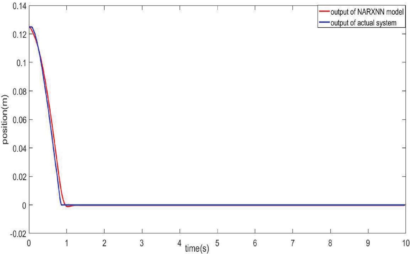
Figure 7 Comparison between output of neural network model and actual system for $u=0V$.

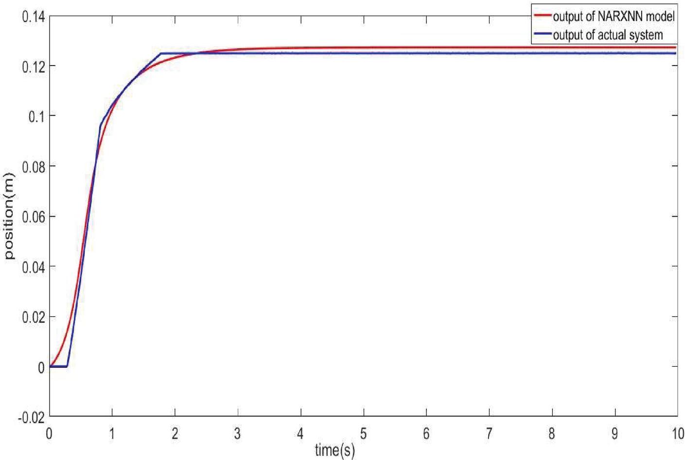
Figure 8 Comparison between output of neural network model and actual system for $u=7V$.

Validating the trained NN model, three different tests responding to variant control inputs $u=0V,u=7V$ and $u=sint(0.5t)V$ have been done and compared to the responses of the real pneumatic servo system as Figures 7–9. In terms of comparison of studies dealing with friction model identification, it worth to mention that a fair comparison had better established in an equal environmental condition, namely stroke length, cylinder diameter, frequency and experimental equipment. Nevertheless, the output error between experimental data and derived neural network proposed in this study is achieved so that compared to (Ning and Bone, 2005) and (Ning and Bone, 2005) the steady-state error decreased as well as it lacks delay, respectively.

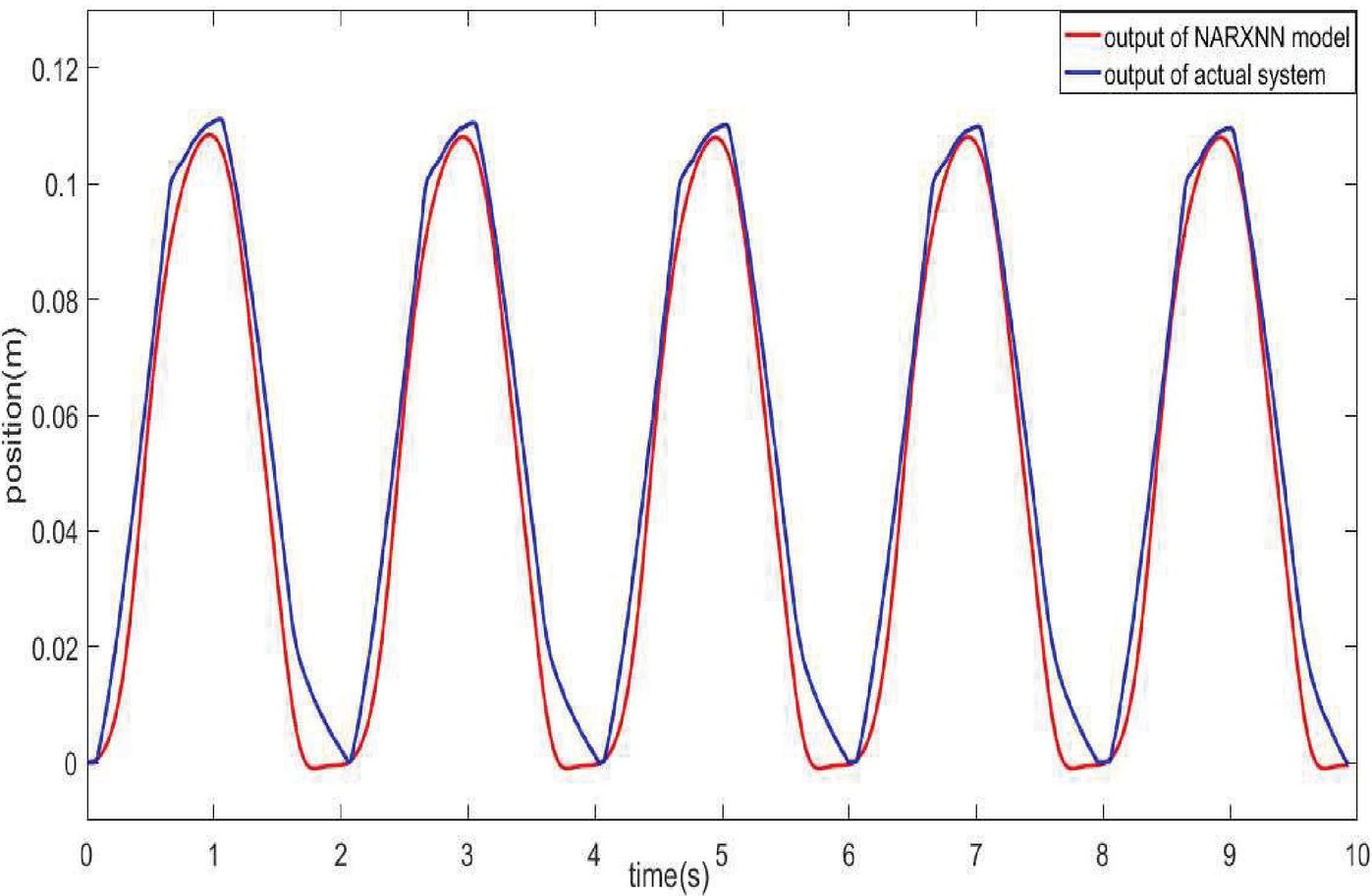
Figure 9 Comparison between output of neural network model and actual system for sinusoidal input.

3 Controller Design and Stability Analysis

3.1 Problem Statement

Generally, a nonlinear, non-affine system can be written as following.

$\begin{array}{c}\hfill {\dot{x}}_i=x_{i+1}\hspace{1em}(i=1,2,\mathrm{\dots },n-1)\hfill \\ \hfill {\dot{x}}_n=F(x,u)+d(t)\hfill \\ \hfill y=x_1\hfill \end{array}$

(9)

For a second order nonlinear pneumatic system with Equations (1)–(7), (9) is obtained for $i=1$, $F=\frac{(P_a{A}_a-P_b{A}_b)-F_l}{M}$ and $d(t)=0$. $X=[x,\dot{x},P_a,P_b]$, and $u$ is a control signal, which is defined in the $\mathrm{\aleph }$ physical bound.

$\mathrm{\aleph }$	$=\{X,u|0.1Mpa\le P\le 0.6Mpa,0\le x_1\le 0.1m,|x_2|\le 0.5m/s,$
	$\mathrm{\hspace{1em}\hspace{1em}}0V\le u\le 10V\}$	(10)

The purpose of the controller design is to establish a proper control signal $u(t)$ directly, so that the output of the pneumatic servo system $y$, in the presence of uncertainty and nonlinear unknown dynamics, is forced to track the reference signal $x_d(t)$ and guaranteed the boundedness of all signals in the closed-loop system.

To design the controller, it is necessary to consider two following assumptions.

Assumption 1: for all $(X,u)\in \mathrm{\aleph }\times R$, the function $f_u=\frac{\partial (F(X,u))}{\partial u}$ is nonsingular and bounded as, $f_u<\mathrm{\Omega }$, where $\mathrm{\Omega }$ is a positive constant.

Assumption 2: The desired trajectory and its time derivatives $x_d,x_d^{(1)},x_d^{(2)}$ are smooth and bounded.

3.2 Feedback Linearization

According to the strategy presented for non-affine systems in (Park et al., 2005), linear feedback control for the pneumatic servo system can be defined as follow,

$$x^{(2)}=F(X,u)=u+\{F(X,u)-u\}=u+\mathrm{\Delta }(X,u)$$

(11)

Where $\mathrm{\Delta }(X,u)=\{F(X,u)-u\}$. The ideal control law can be defined as follows,

$$u^{*}=(x_d^{(2)}-\mathrm{\Delta }(X,u)+K^{T}E)$$

(12)

Where $E={[e,\dot{e}]}^T$, $e=x_d-x,$ $K={[k_0,k_1]}^T$, substituting (12) in (11) gives,

$$\dot{e}=-k_{0}e-k_1\dot{e}$$

(13)

$K$ is chosen in a such way that the (13) is Hurwitz stable, i.e. ${lim}_{t\to \mathrm{\infty }}e=0$ or ${lim}_{t\to \mathrm{\infty }}x=x_d$.

By adding and subtracting optimal control $u^{*}$ in (11), and substituting (12), the dynamic error equation is rewritten as,

$$\dot{e}=-k_{0}e-k_1\dot{e}+(u^{*}-u)$$

(14)

From (14), we obtain the error dynamics in terms of controller parameters which will be mentioned next section. One can obtain compact form of (14) as below,

$$\dot{E}=AE+B[(u^{*}-u)]$$

(15)

Where $A=\left[\begin{array}{cc}\hfill 0\mathit{\hspace{1em}}\hfill & \hfill 1\hfill \\ \hfill -k_0\mathit{\hspace{1em}}\hfill & \hfill -k_1\hfill \end{array}\right]$, $B=\left[\begin{array}{c}\hfill 0\hfill \\ \hfill 1\hfill \end{array}\right]$.

Assumption 3: $E$ belongs to a compact set, $U_e=\{E\in R^n:\parallel E\parallel \le m_e\le \mathrm{\infty }\}$, where $m_e$ is the upper bounds of $E$.

3.3 Direct Adaptive Fuzzy Neural Network (DAFNN) Control Design

Fuzzy Neural Network (FNN) system indicates a Fuzzy logic system (FLS) that is formed as a network. FNN systems exploit both merits of learning ability based on input-output pairs of the Neural Network systems and making decisions based on a rule-base of the Fuzzy logic systems. FNN systems consist of four essential ingredients; fuzzification, fuzzy rule base, inference engine, and defuzzification. To approximate the systems, FLS makes decisions in the inference engine, which combines the “IF-THEN’ rules based on the knowledge of the systems. Takagi-Sugeno Fuzzy inference (Kasabov and Song, 2002) is well-known inference engine, which the consequent parts are formed based on a nonlinear function of the inputs, a simple “IF-THEN’ rule of this kind of system could be presented as below in which its consequent part includes a zero-order function;

$R_j:IF{\widehat{x}}_{1}isA^j{}_{1}and{\widehat{x}}_{2}isA^j{}_2\mathrm{\dots }and{\widehat{x}}_{n}isA^j{}_{n}THEN{\widehat{F}}_j={\theta }_j$

(16)

Where $[{\widehat{x}}_1,{\widehat{x}}_2,\mathrm{\dots },{\widehat{x}}_n],[A^j{}_1,A^j{}_2,\mathrm{\dots },A^j{}_n]$ and ${\widehat{F}}_j$ are the inputs, Fuzzy sets and a zero-order function which its value is equal to ${\theta }_j$ for $j$th rule, respectively.

In this paper, we present a Fuzzy Neural Network (FNN) system to approximate (12) which includes the unknown nonlinear function $\mathrm{\Delta }(X,u)$. Due to this fact that $\mathrm{\Delta }(X,u)$ is a term of the control signal, to generate the output of the FNN control, it needs the control signal $u$ is feedbacked to the controller. Hence, control signal $u$ should be regarded as an input to produce the output of the controller. To overcome this drawback, (Lin and Wai, 2001) Have proposed a Recurrent Neural Network (RNN) control. However, through the recurrent Fuzzy Neural Network (RFNN) systems, a fixed-point problem must be solved in each sample time (Park et al., 2005), which increases the volume of computations and is not appropriate for practical applications. To solve this problem, Theorem 1 is defined.

Theorem 1: (implicit function theorem): Assume that $h:R^n\times R^m\to R^n$ is continuously differentiable at each point $(x,y)$ of an open set $S\subset R^n\times R^m$. Let $(x_0,y_0)$ be a point in $S$ for which $f(x_0,y_0)=0$ and for which the Jacobean matrix $[\frac{\partial f}{\partial a}](x_0,y_0)$ is nonsingular. Then there exist neighbourhood $U\subset R^n$ of $x_0$ and $V\subset R^m$ of $y_0$ such that for each $y\in V$ the equation $f(x,y)=0$ has a unique solution $x\in U$. Moreover, the solution can be given as $x=g(y)$ where $g$ is continuously differentiable at $y=y_0$ (Khalil, 2002).

There is $u^{*}$ that satisfies the following equation.

$$\mathcal{ℒ}(X,v,u^{*})=(v-\mathrm{\Delta }(X,u^{*}))-u^{*}$$

(17)

Where $v=y_d^{(2)}+K^{T}E$.

By considering Assumption 1, non-singularity of $\frac{\partial \mathcal{ℒ}}{\partial u}|u=u^{*}$ is proved.

${{\displaystyle \frac{\partial \mathcal{ℒ}}{\partial u}}|}_{u=u^{*}}$	$={{\displaystyle \frac{\partial ((v-\mathrm{\Delta }(X,u))-u)}{\partial u}}|}_{u=u^{*}}=-{\displaystyle \frac{\partial (F-u)}{\partial u}}-{{\displaystyle \frac{\partial u}{\partial u}}|}_{u=u^{*}}$
	$=-{f_u|}_{u=u^{*}}$	(18)

Thus, according to Theorem 1 there exist a unique $u^{*}(X,v)$ satisfies (17) for all $(X,v)\in \mathrm{\aleph }\times R$. Hence, a feed forward FNN controller which is shown in Figure 10 can be replaced with a RFNN controller. The proposed Fuzzy system differs markedly from the classic one.

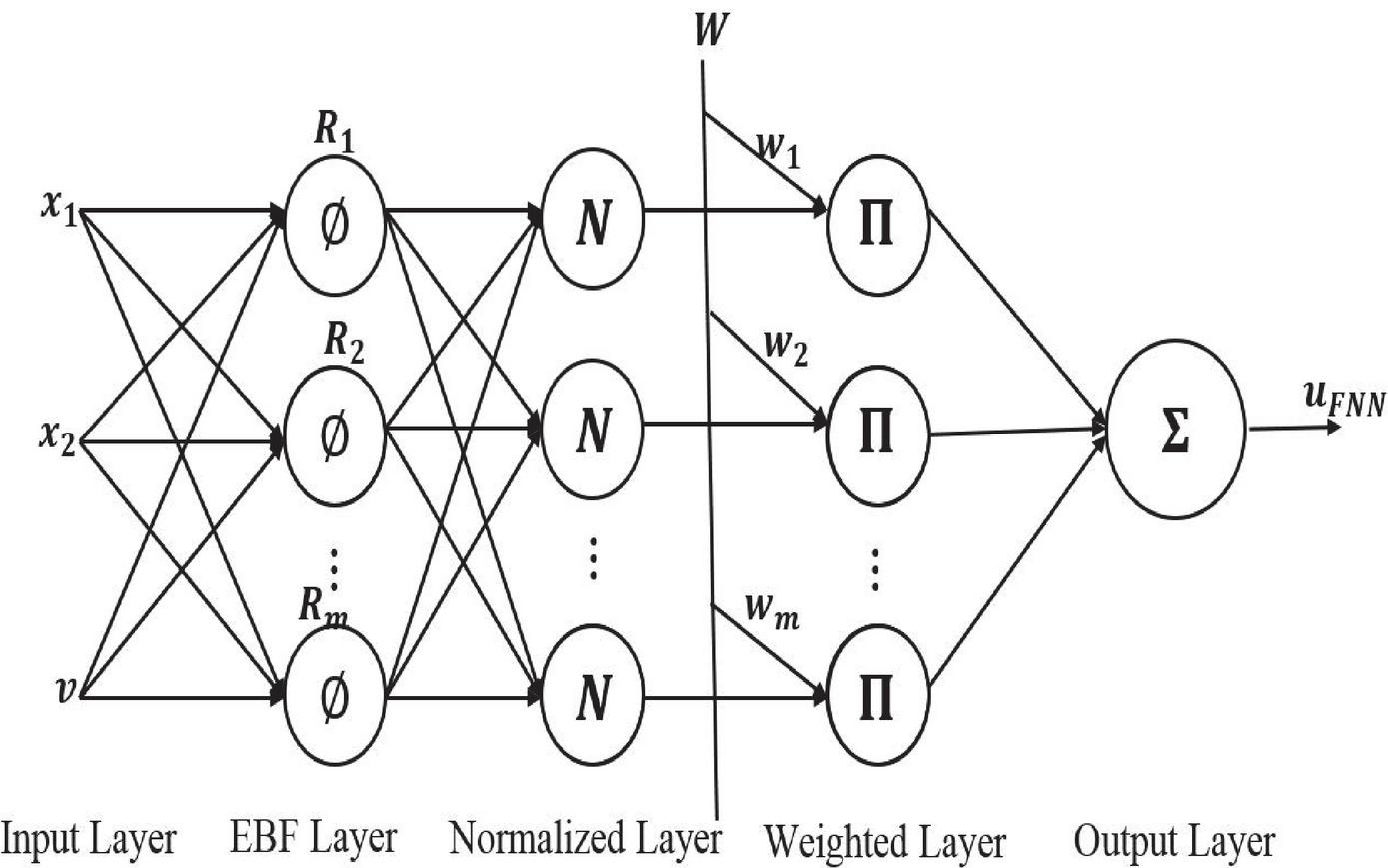
Figure 10 Fuzzy neural network controller structure.

Remark 1: This type of Fuzzy system definition has the capability of being self-structured and the scheme is achievable to implement. FNN system considers each rule (each EBF neuron) as a class and for each input assigns a centre and width of the membership function. In this method, unlike the classic, the number of rules is not obtained based on the number of Fuzzy sets but it is a design parameter.

Remark 2: It is worth to mention that, with regard to indirect adaptive Fuzzy and Neural network (Bounemeur et al., 2018; Theodoridis, et al., 2012) the control law is derived from $u^{*}=\frac{1}{\mathrm{G}(\mathrm{X})}(x_d^{(2)}-\mathrm{F}(\mathrm{X})+K^{T}E)$. The control design, accordingly, necessitates two FNN to be independently employed to approximating $\mathrm{F}(\mathrm{X})$ and $\mathrm{G}(\mathrm{X})$. This measure leads to the scheme being inefficient addressing practical implementation. However, the drawback mentioned above is eradicated, thanks to the direct property of the proposed approach.

As it can be seen in Figure 10, the FNN controller consists of the input layer, the ellipsoidal basis function (EBF) layer which introduced by (Leng et al., 2004), the normalized layer, the weighted layer, and the output layer.

Input layer: This layer provides controller with inputs including position ($x_1$), speed ($x_2$) of the pneumatic actuator and variable $v$.

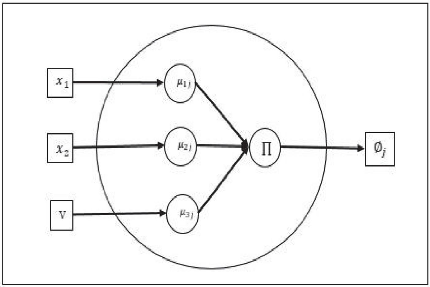
Figure 11 EBF neuron for the $j$th rule schematic.

EBF layer: The $j$th Fuzzy rule can be expressed as EBF Neuron (see Figure 11), in which the membership functions of fuzzy sets are introduced as,

$${\mu }_{ij}=\exp \left(-\frac{{(x_i-c_{ij})}^2}{2{\sigma }_{ij}^2}\right)\mathit{\hspace{1em}}i=1,2,3;j=1,2,\mathrm{\dots },m$$

(19)

Where $m$ is number of neurons and $c_{ij}$, ${\sigma }_{ij}$ are center and width of $i$th input and $j$th neuron, respectively.

By applying the Multiplication T-norm on the fuzzy sets with Gaussian membership function (19) in antecedent part of “If-Then” rules, the output of the EBF layer is obtained as,

$${\mathrm{\varnothing }}_j=\exp \left(-{\int }_{i=1}^3\frac{{(x_i-c_{ij})}^2}{2{\sigma }_{ij}^2}\right)\mathit{\hspace{1em}}j=1,2,\mathrm{\dots },m$$

(20)

Normalized layer: This layer normalize the output of EBF layer, the output of the $j$th neuron in this layer is calculated as follows.

$${\xi }_j=\frac{{\mathrm{\varnothing }}_j}{{\int }_{n=1}^m{\mathrm{\varnothing }}_n}=\frac{\exp \left(-{\int }_{i=1}^3\frac{{(x_i-c_{ij})}^2}{2{\sigma }_{ij}^2}\right)}{{\int }_{n=1}^m\exp \left(-{\int }_{i=1}^3\frac{{(x_i-c_{in})}^2}{2{\sigma }_{in}^2}\right)}\mathit{\hspace{1em}}j=1,2,\mathrm{\dots },m$$

(21)

Weighted layer: In this layer, the outputs of the normalized layer are weighed by weights (the constant parameters in the consequent part of the Takagi-Sugeno fuzzy model.). The outputs of this layer is

$${\mathrm{{\rm Y}}}_j=w_j{\xi }_j\mathit{\hspace{1em}}j=1,2,\mathrm{\dots },m$$

(22)

Output layer: In this layer, the outputs of the weighted layer that were normalized in the third layer are aggregated and form the output of the FNN controller. This layer is the defuzzification section of the fuzzy model. The output can be obtained as follow.

$$u_{FNN}={\int }_{j=1}^m{\mathrm{{\rm Y}}}_j=\frac{{\int }_{j=1}^m{w}_j\exp \left(-{\int }_{i=1}^3\frac{{(x_i-c_{ij})}^2}{2{\sigma }_{ij}^2}\right)}{{\int }_{n=1}^m\exp \left(-{\int }_{i=1}^3\frac{{(x_i-c_{in})}^2}{2{\sigma }_{in}^2}\right)}$$

(23)

We can rewrite (23) in matrix form.

$$u_{FNN}=W^{T}Q([x_1,x_2,v]|C,\sigma )$$

(24)

Where,

$W$	$={[w_1,w_2,\mathrm{\dots }{w}_m]}^T\in R^{m\times 1},$	(25)
$Q$	$={[{\xi }_1,{\xi }_2,\mathrm{\dots },{\xi }_m]}^T\in R^{m\times 1},$	(26)
$C$	$=[c_{11},c_{12},\mathrm{\dots },c_{1m},c_{21},c_{22},\mathrm{\dots },c_{2m},c_{31},c_{32},\mathrm{\dots },c_{3m}]\in R^{1\times (3m)},$	(27)
$\sigma$	$=[{\sigma }_{11},{\sigma }_{12},\mathrm{\dots },{\sigma }_{1m},{\sigma }_{21},{\sigma }_{22},\mathrm{\dots },{\sigma }_{2m},{\sigma }_{31},{\sigma }_{32},\mathrm{\dots },{\sigma }_{3m}]\in R^{1\times (3m)}.$	(28)

An optimal FNN can be obtained to approximate the control signal.

$$u^{*}=W^{*}{}^T{Q}^{*}(C^{*},{\sigma }^{*})+\delta ([x_1,x_2,v])$$

(29)

Where $\delta ([x_1,x_2,v])$ is approximation error and $|\delta |\le \mathrm{\beth }$, which $\mathrm{\beth }$ is constant parameter, and $W^{*}$ and $Q^{*}(C^{*},{\sigma }^{*})$ are the optimal parameters of $W$ and $Q(C,\sigma )$, respectively.

Assumption 4: The optimal parameters of controller are obtained so that $[W^{*},C^{*},{\sigma }^{*}]=argmi{n}_{W\in m_w,C\in m_c,\sigma \in m_{\sigma }}[su{p}_{[x_1,x_2,\mathrm{v}]\in \mathrm{\aleph }\times R}|u^{*}([x_1,x_2,\mathrm{v}])-u_{FNN}([x_1,x_2,\mathrm{v}]|w,c,\sigma )]$ , with the bounded regions of parameters as,

$m_w$	$=\{W\in R^n:\parallel W\parallel \le \beta \},m_c=\{C\in R^n:\parallel C\parallel \le \mathrm{{\rm Y}}\},$
$m_{\sigma }$	$=\{\sigma \in R^n:\parallel \sigma \parallel \le \mathrm{\Omega }\},$
$m_Q$	$=\{Q\in R^n:\parallel Q\parallel \le \chi \},m_{\frac{\partial Q}{\partial C}}=\{{\displaystyle \frac{\partial Q}{\partial C}}\in R^n:\parallel {\displaystyle \frac{\partial Q}{\partial C}}\parallel \le {\chi }_1\},$
$m_{\frac{\partial Q}{\partial \sigma }}$	$=\{{\displaystyle \frac{\partial Q}{\partial \sigma }}\in R^n:\parallel {\displaystyle \frac{\partial Q}{\partial \sigma }}\parallel \le {\chi }_2\}$	(30)

Where, $\beta ,\mathrm{{\rm Y}},\mathrm{\Omega },\chi$ are the raduise of parameters region.

To obtain adaptive laws, the dynamic error equation (15) is rewritten in terms of the parameter variations from their optimal values.

$\dot{E}=AE+B\left[\left({\tilde{W}}^{T}Q+W^T{\displaystyle \frac{\partial Q}{\partial C}}\tilde{C}+W^T{\displaystyle \frac{\partial Q}{\partial \sigma }}\tilde{\sigma }+\epsilon \right)\right]$

Where $\tilde{W}=W^{*}-W,\tilde{C}=C^{*}-C,\tilde{\sigma }={\sigma }^{*}-\sigma$ and $\epsilon =\delta ([x_1,x_2,\mathrm{v}])+W^{T}h(O^2)+{\tilde{W}}^T\tilde{Q}$.

Proof: By substituting, (24) and (29) in (15), the following equation is obtained.

$$\dot{E}=AE+B[(W^{*}{}^T{Q}^{*}-W^{T}Q+\delta )]$$

(32)

By adding and subtracting $W^T{Q}^{*}$ and ${\tilde{W}}^{T}Q$ in (32) and simplification, following equation is derived.

$$\dot{E}=AE+B[({\tilde{W}}^T\tilde{Q}+{\tilde{W}}^{T}Q+W^T\tilde{Q}+\delta )]$$

(33)

Based work of (Han et al., 2017), Taylor series technique is used to linearize the two-variable nonlinear function $Q^{*}$ respect to $Q$.

$Q^{*}$	$=Q+{\displaystyle \frac{\partial Q}{\partial C}}{(C^{*}-C)}^T+{\displaystyle \frac{\partial Q}{\partial \sigma }}{({\sigma }^{*}-\sigma )}^T$
	$\mathrm{\hspace{1em}}+h(O^2)\stackrel{yields}{\to }\tilde{Q}={\displaystyle \frac{\partial Q}{\partial C}}{\tilde{C}}^T+{\displaystyle \frac{\partial Q}{\partial \sigma }}{\tilde{\sigma }}^T+h(O^2)$	(34)

Where,

${\displaystyle \frac{\partial Q}{\partial C}}=\left[\begin{array}{ccc}\hfill {\displaystyle \frac{\partial Q_1}{\partial c_{11}}},{\displaystyle \frac{\partial Q_1}{\partial c_{12}}},\mathrm{\dots },{\displaystyle \frac{\partial Q_1}{\partial c_{1m}}}\mathit{\hspace{1em}}\hfill & \hfill \mathrm{\cdots }\mathit{\hspace{1em}}\hfill & \hfill {\displaystyle \frac{\partial Q_1}{\partial c_{31}}},{\displaystyle \frac{\partial Q_1}{\partial c_{32}}},\mathrm{\dots },{\displaystyle \frac{\partial Q_1}{\partial c_{3m}}}\hfill \\ \hfill {\displaystyle \frac{\partial Q_2}{\partial c_{11}}},{\displaystyle \frac{\partial Q_2}{\partial c_{12}}},\mathrm{\dots },{\displaystyle \frac{\partial Q_2}{\partial c_{1m}}}\mathit{\hspace{1em}}\hfill & \hfill \mathrm{\dots }\mathit{\hspace{1em}}\hfill & \hfill {\displaystyle \frac{\partial Q_2}{\partial c_{31}}},{\displaystyle \frac{\partial Q_2}{\partial c_{32}}},\mathrm{\dots },{\displaystyle \frac{\partial Q_2}{\partial c_{3m}}}\hfill \\ \hfill \mathrm{⋮}\mathit{\hspace{1em}}\hfill & \hfill \mathrm{\ddots }\mathit{\hspace{1em}}\hfill & \hfill \mathrm{⋮}\hfill \\ \hfill {\displaystyle \frac{\partial Q_m}{\partial c_{11}}},{\displaystyle \frac{\partial Q_m}{\partial c_{12}}},\mathrm{\dots },{\displaystyle \frac{\partial Q_m}{\partial c_{1m}}}\mathit{\hspace{1em}}\hfill & \hfill \mathrm{\cdots }\mathit{\hspace{1em}}\hfill & \hfill {\displaystyle \frac{\partial Q_m}{\partial c_{31}}},{\displaystyle \frac{\partial Q_m}{\partial c_{32}}},\mathrm{\dots },{\displaystyle \frac{\partial Q_m}{\partial c_{3m}}}\hfill \end{array}\right]\in R^{m\times (3m)}$

(35)

${\displaystyle \frac{\partial Q}{\partial \sigma }}=\left[\begin{array}{ccc}\hfill {\displaystyle \frac{\partial Q_1}{\partial {\sigma }_{11}}},{\displaystyle \frac{\partial Q_1}{\partial {\sigma }_{12}}},\mathrm{\dots },{\displaystyle \frac{\partial Q_1}{\partial {\sigma }_{1m}}}\mathit{\hspace{1em}}\hfill & \hfill \mathrm{\cdots }\mathit{\hspace{1em}}\hfill & \hfill {\displaystyle \frac{\partial Q_1}{\partial {\sigma }_{31}}},{\displaystyle \frac{\partial Q_1}{\partial {\sigma }_{32}}},\mathrm{\dots },{\displaystyle \frac{\partial Q_1}{\partial {\sigma }_{3m}}}\hfill \\ \hfill {\displaystyle \frac{\partial Q_2}{\partial {\sigma }_{11}}},{\displaystyle \frac{\partial Q_2}{\partial {\sigma }_{12}}},\mathrm{\dots },{\displaystyle \frac{\partial Q_2}{\partial {\sigma }_{1m}}}\mathit{\hspace{1em}}\hfill & \hfill \mathrm{\dots }\mathit{\hspace{1em}}\hfill & \hfill {\displaystyle \frac{\partial Q_2}{\partial {\sigma }_{31}}},{\displaystyle \frac{\partial Q_2}{\partial {\sigma }_{32}}},\mathrm{\dots },{\displaystyle \frac{\partial Q_2}{\partial {\sigma }_{3m}}}\hfill \\ \hfill \mathrm{⋮}\mathit{\hspace{1em}}\hfill & \hfill \mathrm{\ddots }\mathit{\hspace{1em}}\hfill & \hfill \mathrm{⋮}\hfill \\ \hfill {\displaystyle \frac{\partial Q_m}{\partial {\sigma }_{11}}},{\displaystyle \frac{\partial Q_m}{\partial {\sigma }_{12}}},\mathrm{\dots },{\displaystyle \frac{\partial Q_m}{\partial {\sigma }_{1m}}}\mathit{\hspace{1em}}\hfill & \hfill \mathrm{\cdots }\mathit{\hspace{1em}}\hfill & \hfill {\displaystyle \frac{\partial Q_m}{\partial {\sigma }_{31}}},{\displaystyle \frac{\partial Q_m}{\partial {\sigma }_{32}}},\mathrm{\dots },{\displaystyle \frac{\partial Q_m}{\partial {\sigma }_{3m}}}\hfill \end{array}\right]\in R^{m\times (3m)}$

(36)

And

${\displaystyle \frac{\partial Q_j}{\partial c_{ij}}}$	$={\displaystyle \frac{x_i-c_{ij}}{{\sigma }_{ij}^2}}({\xi }_j-{\xi }_j^2)$	(37)
${\displaystyle \frac{\partial Q_j}{\partial {\sigma }_{ij}}}$	$={\displaystyle \frac{{(x_i-c_{ij})}^2}{{\sigma }_{ij}^3}}({\xi }_j-{\xi }_j^2)$	(38)

By substituting, (34) in (33), (31) is derived. $\mathrm{■}$

Theorem 2: For the non-linear, non-affine system (9) with control law (12) which is derived through a direct FNN control (23), if assumptions are satisfied, the close-loop system is stable, the parameters of DAFNN are bounded, and tracking trajectory error tends to zero, i.e. ${lim}_{t\to \mathrm{\infty }}E\to 0$.

Proof: Define The Lyapunov function as,

$$V=\frac{1}{2}{E}^{T}PE+\frac{1}{2{\gamma }_w}{\tilde{W}}^T\tilde{W}+\frac{1}{2{\gamma }_c}{\tilde{C}}^T\tilde{C}+\frac{1}{2{\gamma }_{\sigma }}{\tilde{\sigma }}^T\tilde{\sigma }$$

(39)

Where ${\gamma }_w,{\gamma }_c$, and ${\gamma }_{\sigma }$ are positive learning rates and $P$ is a $n\times n$ symmetric matrix which satisfies the Lyapunov equation.

$$A^{T}P+PA=-q$$

(40)

Where $q$ is an arbitrary $n\times n$ positive definite matrix. Differentiating (39) respect time gives,

$\dot{V}$	$={\displaystyle \frac{1}{2}}{E}^T(A^{T}P+PA)E+{\displaystyle \frac{1}{2}}({({\tilde{W}}^{T}Q)}^T{B}^{T}PE+E^{T}PB{\tilde{W}}^{T}Q)$
	$\mathrm{\hspace{1em}}+{\displaystyle \frac{1}{2}}\left({\left(W^T{\displaystyle \frac{\partial Q}{\partial C}}{\tilde{C}}^T\right)}^T{B}^{T}PE+E^{T}PB{W}^T{\displaystyle \frac{\partial Q}{\partial C}}{\tilde{C}}^T\right)$
	$\mathrm{\hspace{1em}}+{\displaystyle \frac{1}{2}}\left({\left(W^T{\displaystyle \frac{\partial Q}{\partial \sigma }}{\tilde{\sigma }}^T\right)}^T{B}^{T}PE+E^{T}PB{W}^T{\displaystyle \frac{\partial Q}{\partial \sigma }}{\tilde{\sigma }}^T\right)$
	$\mathrm{\hspace{1em}}+{\displaystyle \frac{1}{2}}\left({(\epsilon )}^T{B}^{T}PE+E^{T}PB\epsilon \right)-{\displaystyle \frac{1}{{\gamma }_w}}{\tilde{W}}^T\dot{W}-{\displaystyle \frac{1}{{\gamma }_c}}{\tilde{C}}^T\dot{C}-{\displaystyle \frac{1}{{\gamma }_{\sigma }}}{\tilde{\sigma }}^T\sigma$	(41)

By applying this fact that,

$E^{T}PB{\tilde{W}}^{T}Q$	$={({\tilde{W}}^{T}Q)}^T{B}^{T}PE$	(42)
$E^{T}PB{W}^T{\displaystyle \frac{\partial Q}{\partial C}}{\tilde{C}}^T$	$={\left(W^T{\displaystyle \frac{\partial Q}{\partial C}}{\tilde{C}}^T\right)}^T{B}^{T}PE$	(43)
$E^{T}PB{W}^T{\displaystyle \frac{\partial Q}{\partial \sigma }}{\tilde{\sigma }}^T$	$={\left(W^T{\displaystyle \frac{\partial Q}{\partial \sigma }}{\tilde{\sigma }}^T\right)}^T{B}^{T}PE$	(44)
$E^{T}PB\epsilon$	$={(\epsilon )}^T{B}^{T}PE$	(45)

(41) is rewritten as,

$\dot{V}$	$=-{\displaystyle \frac{1}{2}}{E}^T(q)E+\left(E^{T}PBQ-{\displaystyle \frac{1}{{\gamma }_w}}\dot{W}\right){\tilde{W}}^T$
	$\mathrm{\hspace{1em}}+\left(E^{T}PB{W}^T{\displaystyle \frac{\partial Q}{\partial C}}-{\displaystyle \frac{1}{{\gamma }_c}}\dot{C}\right){\tilde{C}}^T$
	$\mathrm{\hspace{1em}}+\left(E^{T}PB{W}^T{\displaystyle \frac{\partial Q}{\partial \sigma }}-{\displaystyle \frac{1}{{\gamma }_{\sigma }}}\dot{\sigma }\right){\tilde{\sigma }}^T+E^{T}PB\epsilon$	(46)

choose the adaptive laws as below,

$\dot{W}$	$={\gamma }_w{E}^{T}PBQ$	(47)
$\dot{C}$	$={\gamma }_c{E}^{T}PB{W}^T{\displaystyle \frac{\partial Q}{\partial C}}$	(48)
$\dot{\sigma }$	$={\gamma }_{\sigma }{E}^{T}PB{W}^T{\displaystyle \frac{\partial Q}{\partial \sigma }}$	(49)

Then the following can be obtained,

$$\dot{V}=-\frac{1}{2}{E}^T\left(q\right)E+E^{T}PB\epsilon$$

(50)

According to (34), the following inequality always exists.

$W^{T}h(O^2)$	$\le \parallel W^T\parallel |h(O^2)|\le \parallel W^T\parallel (\parallel Q^{*}\parallel +\parallel Q\parallel +\parallel {\displaystyle \frac{\partial Q}{\partial C}}\parallel \parallel C^{*}\parallel$
	$\mathrm{\hspace{1em}}+\parallel {\displaystyle \frac{\partial Q}{\partial C}}\parallel \parallel C\parallel +\parallel {\displaystyle \frac{\partial Q}{\partial \sigma }}\parallel \parallel {\sigma }^{*}\parallel +\parallel {\displaystyle \frac{\partial Q}{\partial \sigma }}\parallel \parallel \sigma \parallel )$	(51)

As well as we can write,

${\tilde{W}}^T\tilde{Q}\le \left|{\tilde{W}}^T\tilde{Q}\right|\le \parallel W^{*}\parallel \parallel Q^{*}\parallel +\parallel W^{*}\parallel \parallel Q\parallel +\parallel W\parallel \parallel Q^{*}\parallel +\parallel W\parallel \parallel Q\parallel$

(52)

Using Assumption 4 we have,

$W^{T}h(O^2)\le \mathrm{\Gamma }$

(53)

And

${\tilde{W}}^T\tilde{Q}\le \mathrm{\Lambda }$

(54)

Where $\mathrm{\Gamma }=c1\beta +\beta \chi +c2\beta {\chi }_1+\beta {\chi }_1\mathrm{{\rm Y}}+c3\beta {\chi }_2+\beta {\chi }_1\mathrm{\Omega }$ and $\mathrm{\Lambda }=c4c1+c4\chi +\beta c1+\beta \chi$.

By substituting (53), (54) we have,

$\dot{V}$	$\le -{\displaystyle \frac{1}{2}}{E}^T(q)E+E^{T}PB(\delta ([x_1,x_2,\mathrm{v}])+\mathrm{\Gamma }+\mathrm{\Lambda })$
	$\le -{\displaystyle \frac{1}{2}}{E}^T(q)E+E^{T}PB(\mathrm{\beth }+\mathrm{\Gamma }+\mathrm{\Lambda })$	(55)

By using young’s inequality for the second terms we can have,

$E^{T}PB\mathrm{\beth }\le {\displaystyle \frac{1}{2}}{E}^{T}PB{B}^T{P}^{T}E+{\displaystyle \frac{1}{2}}{\mathrm{\beth }}^2$	(56)
$E^{T}PB\mathrm{\Gamma }\le {\displaystyle \frac{1}{2}}{E}^{T}PB{B}^T{P}^{T}E+{\displaystyle \frac{1}{2}}{\mathrm{\Gamma }}^2$	(57)
$E^{T}PB\mathrm{\Lambda }\le {\displaystyle \frac{1}{2}}{E}^{T}PB{B}^T{P}^{T}E+{\displaystyle \frac{1}{2}}{\mathrm{\Lambda }}^2$	(58)

Then (55) is rewritten as following,

$$\dot{V}\le -\frac{1}{2}{E}^T(\mathrm{\Phi })E+\frac{1}{2}({\mathrm{\beth }}^2+{\mathrm{\Gamma }}^2+{\mathrm{\Lambda }}^2)$$

(59)

Where,

$$-\mathrm{\Phi }=-q+3PB{B}^T{P}^T$$

(60)

By using this fact, $-E^T(\mathrm{\Phi })E\le -{\lambda }_{min}(\mathrm{\Phi }){\parallel E\parallel }^2$, (59) rewritten as below,

$$\dot{V}\le -\frac{1}{2}{\lambda }_{min}(\mathrm{\Phi }){\parallel E\parallel }^2+\frac{1}{2}({\mathrm{\beth }}^2+{\mathrm{\Gamma }}^2+{\mathrm{\Lambda }}^2)$$

(61)

Let $\alpha ={\lambda }_{min}(\mathrm{\Phi }{\mathrm{P}}^{-1})$ and $\pi =\frac{1}{2}({\mathrm{\beth }}^2+{\mathrm{\Gamma }}^2+{\mathrm{\Lambda }}^2)$. Then (61) is obtained as,

$$\dot{V}\le -\alpha V+\pi$$

(62)

By integrating over [0, tf] from (62) we have,

$$V\le e^{-\alpha t}\left(V(0)-\frac{\pi }{\alpha }\right)+\frac{\pi }{\alpha }$$

(63)

As a result it can be said that $\parallel E\parallel \le \sqrt{2\frac{e^{-\alpha t}(V(0)-\frac{\pi }{\alpha })+\frac{\pi }{\alpha }}{{\lambda }_{min}(P)}},$ therefore $E$ is bound and Assumption 3 is satisfied, i.e

$$U_e=\{E\in R^n:\parallel E\parallel \le \sqrt{2\frac{e^{-\alpha t}\left(V(0)-\frac{\pi }{\alpha }\right)+\frac{\pi }{\alpha }}{{\lambda }_{min}(P)}}\le \mathrm{\infty }\}$$

and the proof is completed. $\mathrm{■}$

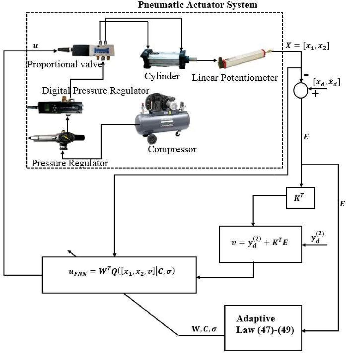
Figure 12 Block diagram for control system.

In Figure 12, the block diagram for the control system is shown. The steps of the controller design algorithm are briefly outlined in a five steps,

• Initial position and velocity of the pneumatic actuator system is determined

• The initial value of $W,C,$ and $\sigma$ is specified.

• From Equation (23), the control signal is obtained.

• The control signal is applied to the pneumatic actuator system and feed-backed error vector $E$ is characterized.

• From Equations (47)–(49) the controller parameters are updated.

4 Simulation and Experimental Results

In this paper, first, an accurate non-linear autoregressive exogenous model with Neural network (NARXNN) for the practical pneumatic system was extracted. Secondly, a direct adaptive Fuzzy Neural Network (DAFNN) controller for control the output of NARXNN was simulated; finally, the controller is implemented on the practical pneumatic servo system with unknown dynamics. To evaluate the control simulation results, several comparisons with practical results are done.

The controller parameters are updated by hybrid method, i.e. the weight parameters of FNN (the constant parameters of consequent part of Takagi-Sugeno Fuzzy model) and the EBF neurons parameters (parameters of antecedent part of Fuzzy rules) are tuned simultaneously.

The initial position and velocity of the pneumatic servo system are $x(0)=0,\dot{x}(0)=0$ and initial value of controller’s parameters are

$W(0)$	$=[0]\in R^{3\times 1},$
$C(0)$	$=[0.847,0.9058,0.127,0.9134,0.6324,0.975,0.2785,$
	$\mathrm{\hspace{1em}}0.5469,0.9]$

and $\sigma (0)=[0.6]\in R^{1\times 9}$, as well as the design parameters are selected as, $K={[1,1]}^T$, $q=\left[\begin{array}{cc}\hfill 30\mathit{\hspace{1em}}\hfill & \hfill 0\hfill \\ \hfill 0\mathit{\hspace{1em}}\hfill & \hfill 5\hfill \end{array}\right]$ and ${\gamma }_w={\gamma }_c={\gamma }_{\sigma }=50$, also in term of practical control system implement, the sampling rate of the PCI1710U card is selected so that data acquiring is done each $0.01s$ interval.

The performance of the (DAFNN) controller significantly depends on the number of EBF neurons. If EBF neurons are chosen large, the controller’s complexity could arise result in practical implementation being far out of reach; On the other hand, if it is selected small, the controller accuracy decreases. Turning to a feasible solution, one can use the self-structure fuzzy neural network system. However, in this paper, three EBF neurons are chosen. In following, to examine the performance of the controller, two aspects of control problems, including trajectory tracking control and robustness test against the mass parameter change are investigated.

4.1 Trajectory Tracking Control

The performance of the control scheme, tracking two distinct trajectory is investigated. As the achievable workspace for the piston is limited to the span of [0–0.125 m], the trajectories are considered as bellow.

$case(1):y_d$	$=0.05(\sin (t)+1)$	(64)
$case(2):y_d$	$=0.0284(\sin (t)+\cos (0.5t)+1.7602)$	(65)

All results of this section are obtained for the condition in which the nominal mass and supply pressure are selected 18 kg and 0.6 MPa, respectively. The control system output (the controlled system’s position of the piston), the control signal, tracking error, and zoomed in error are shown in Figure 13. As can be seen from Figure 13(a), the practical and simulation results properly track the desired trajectory. The errors (Figures 13(c) and 13(d)) are obtained $\pm$1.3mm and $\pm$1mm, respectively, which indicate that the controller performs a satisfactory ability in tracking the desired trajectory expressed by the case (1). Moreover, the performance for the controller tracking case (2), has been made. The control system output (the controlled system’s position of the piston), the control signal, and the tracking error are shown in Figure 14. According to Figure 14(d), the tracking error for the practical and simulation control system is $\pm$1mm and $\pm$0.5mm, respectively.

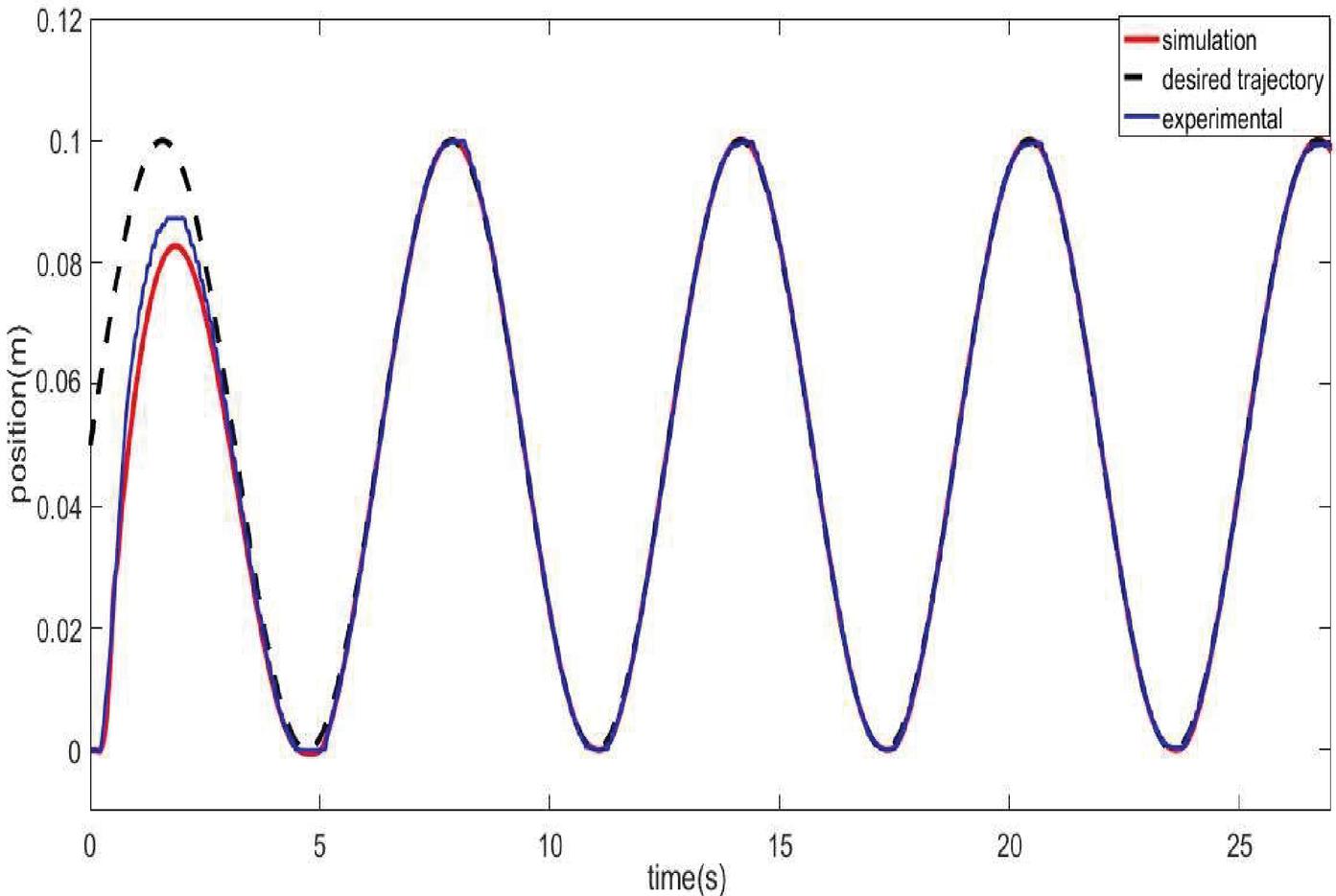
Figure 13(a): Experimental output and simulation output of (DAFNN) controller with hybrid tuning for tracking case (1).

Figure 13(b): Experimental system and simulation control signal of (DAFNN) controller with hybrid tuning for tracking case (1).

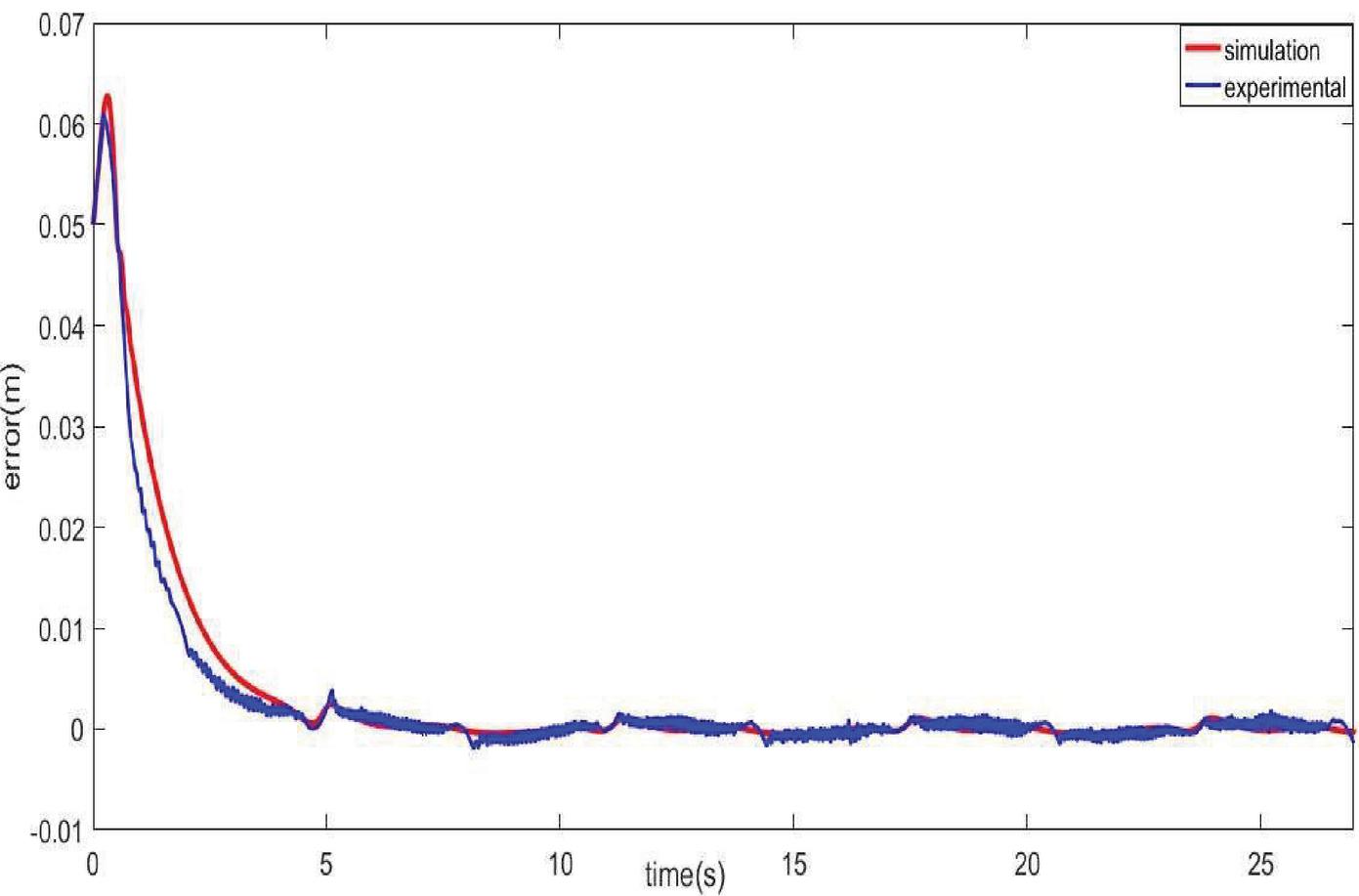
Figure 13(c): Experimental and simulation trajectory tracking error of (DAFNN) controller with hybrid tuning for tracking case (1).

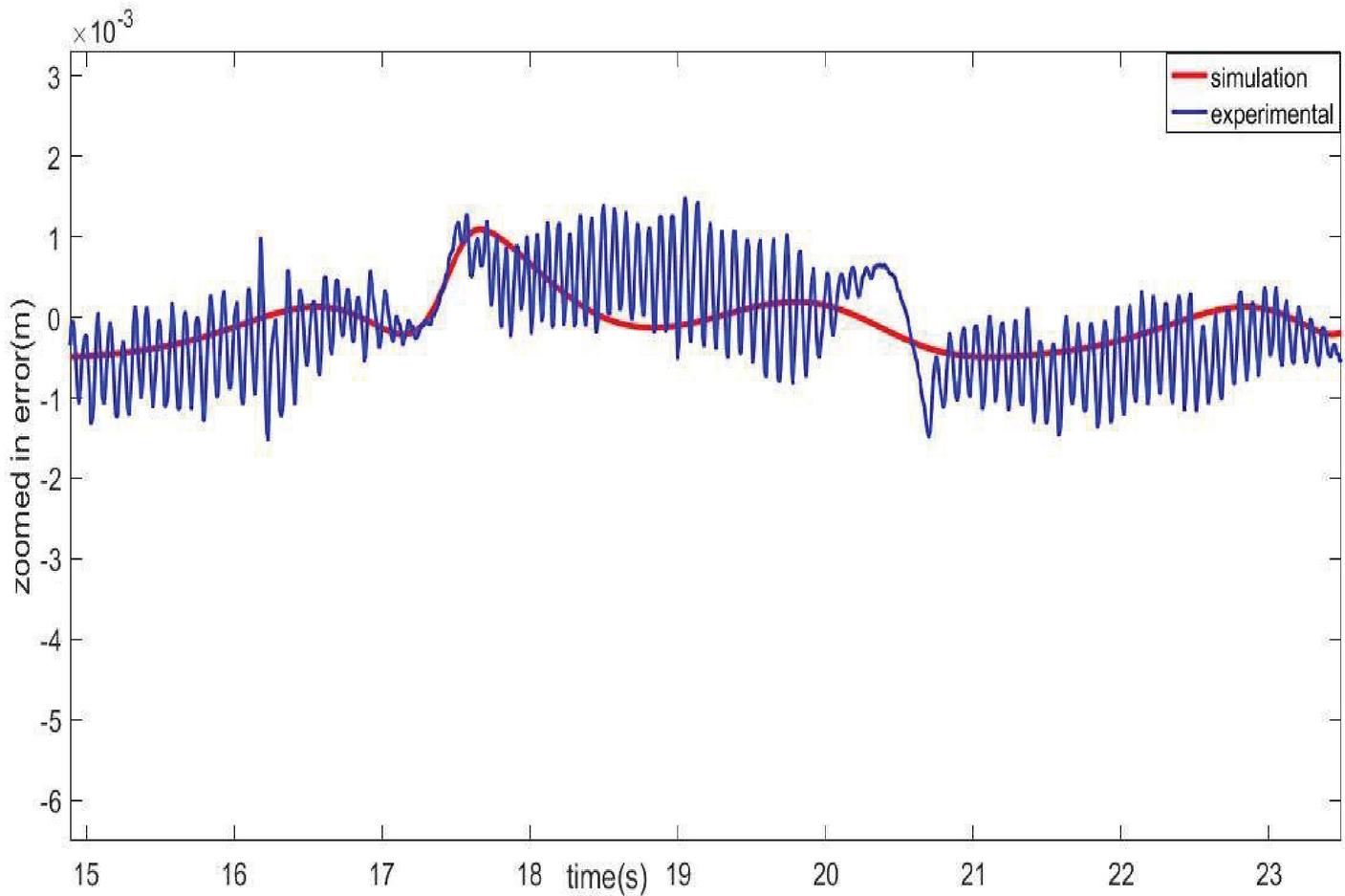
Figure 13(d): Experimental and simulation zoomed in trajectory tracking error of (DAFNN) controller with hybrid tuning for tracking case (1).

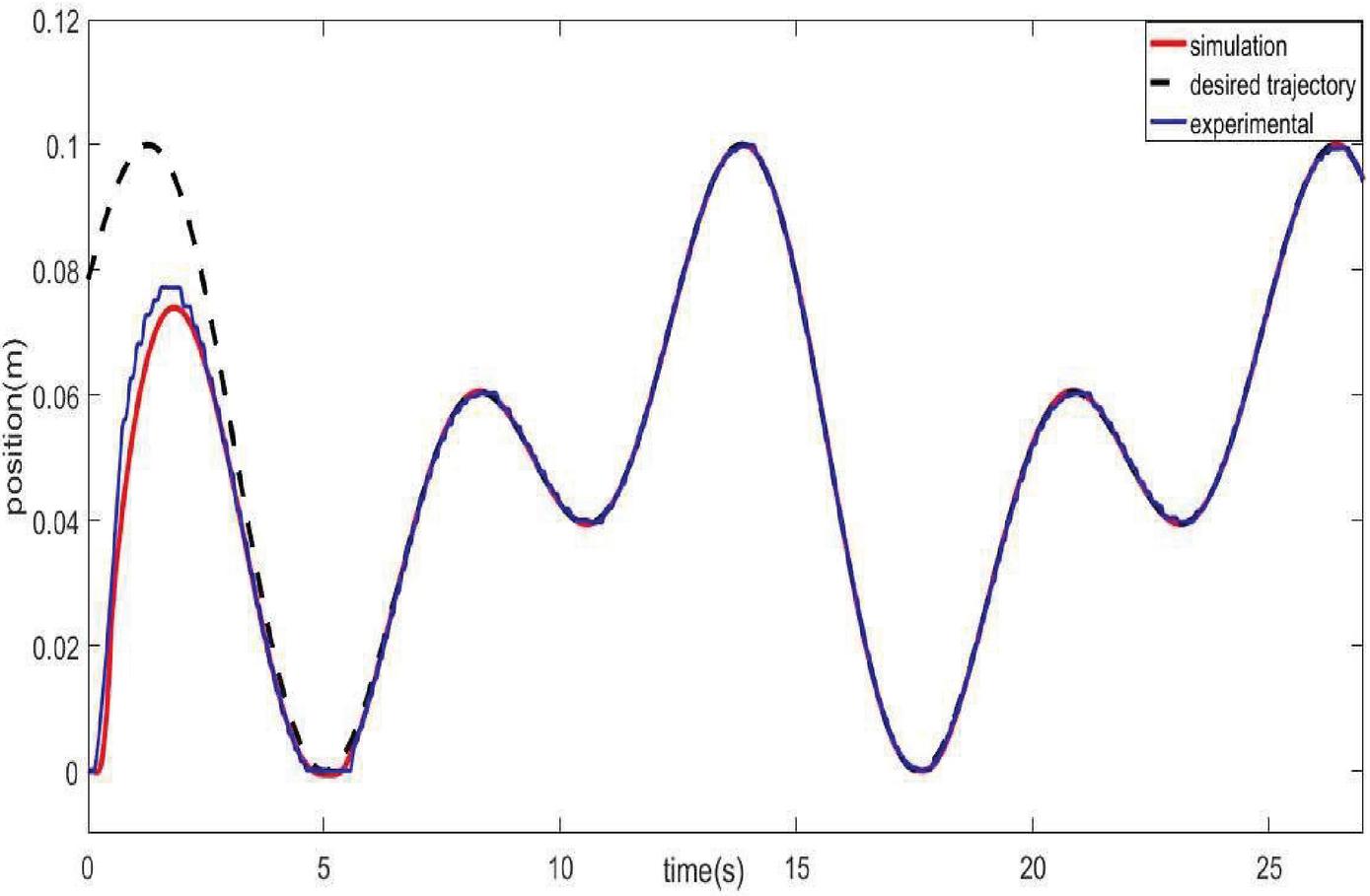
Figure 14(a): Experimental output and simulation output of (DAFNN) controller with hybrid tuning for tracking case (2).

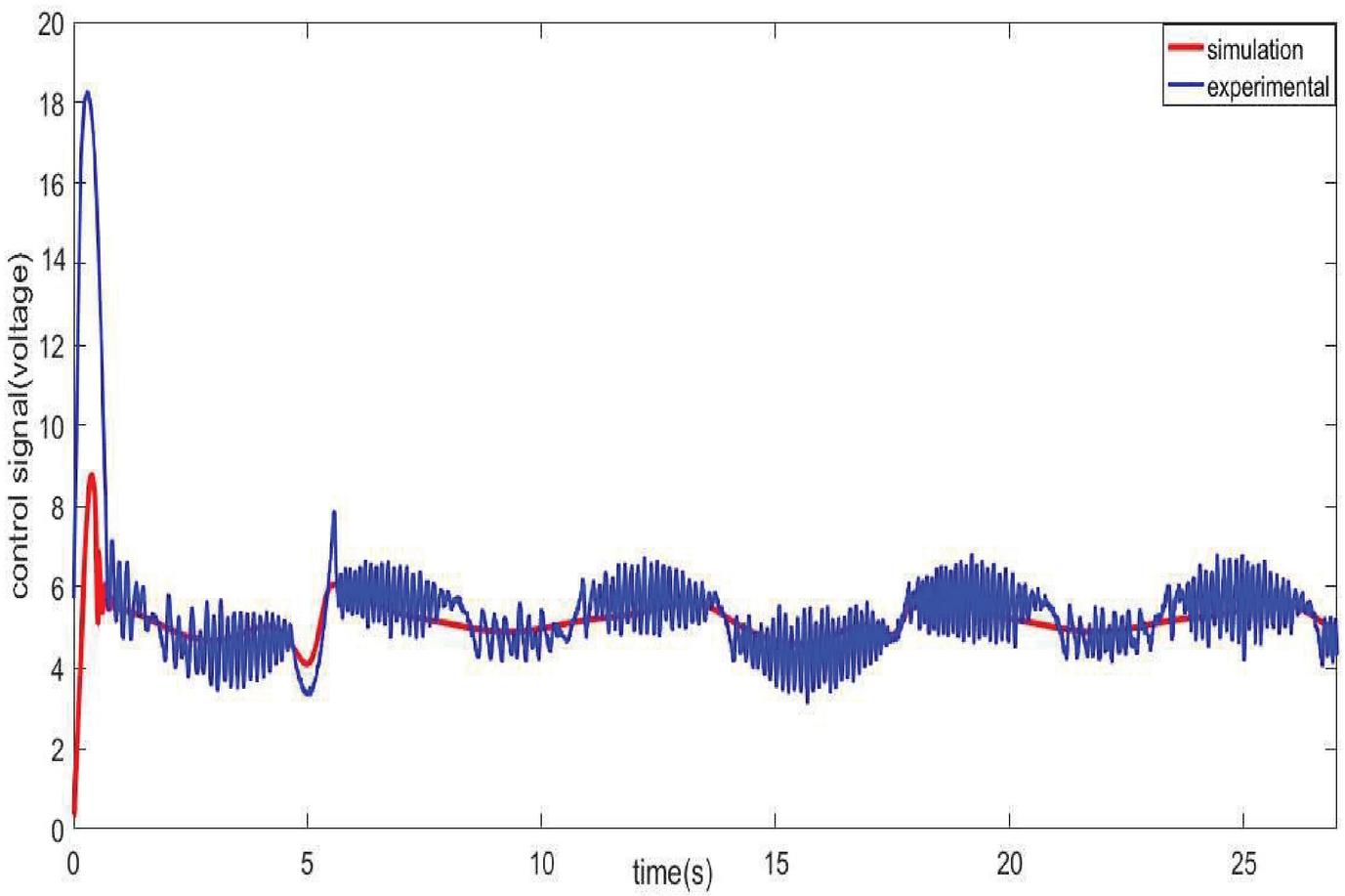
Figure 14(b): Experimental system and simulation control signal of (DAFNN) controller with hybrid tuning for tracking case (2).

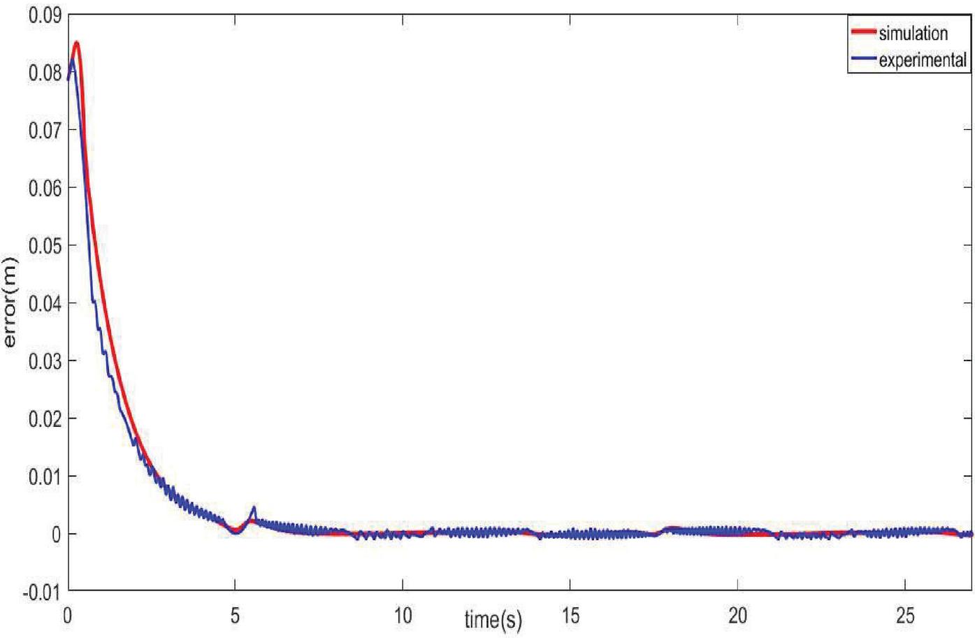
Figure 14(c): Experimental and simulation trajectory tracking error of (DAFNN) controller with hybrid tuning for tracking case (2).

Figure 14(d): Experimental and simulation zoomed in trajectory tracking error of (DAFNN) controller with hybrid tuning for tracking case (2).

The mentioned results are obtained for the case in which the parameter adjustments are accomplished with a hybrid method. To investigate the effect of hybrid adjustment for the controller parameters on tracking error, the presented results have been compared with a situation in which only the weights of FNN controller (Phan and Gale, 2008) (parameters of consequent of Takagi-Sugeno fuzzy rules) are updated.

Practical and simulation results for controller which parameters are updated by weight adjustment method for the desired trajectory case (1) and case (2) are shown in Figures 15 and 16, respectively. As Figure 15(d) and 16(d), in this method, the tracking error of the practical control system and the simulation for case (1) is $\pm$2.5mm and $\pm$3mm, and for the case (2) is $\pm$3.5mm and $\pm$2mm, respectively.

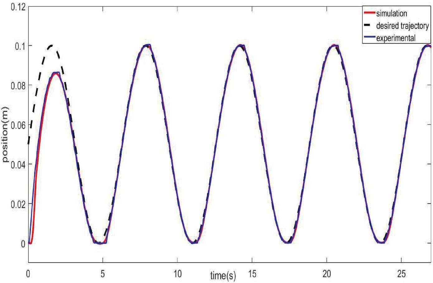
Figure 15(a): Experimental output and simulation output of (DAFNN) controller with the weight parameters tuning for tracking case (1).

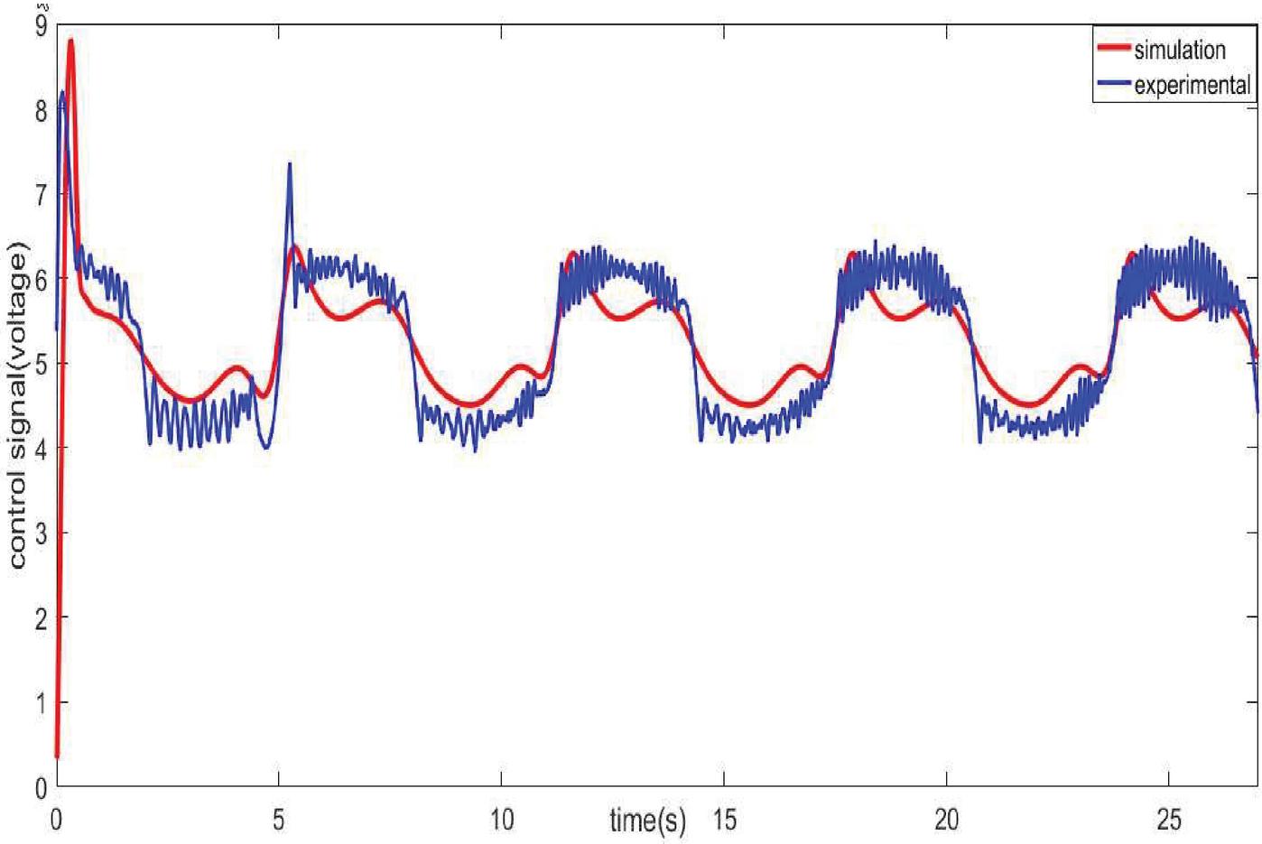
Figure 15(b): Experimental system and simulation control signal of (DAFNN) controller with the weight parameters tuning for tracking case (1).

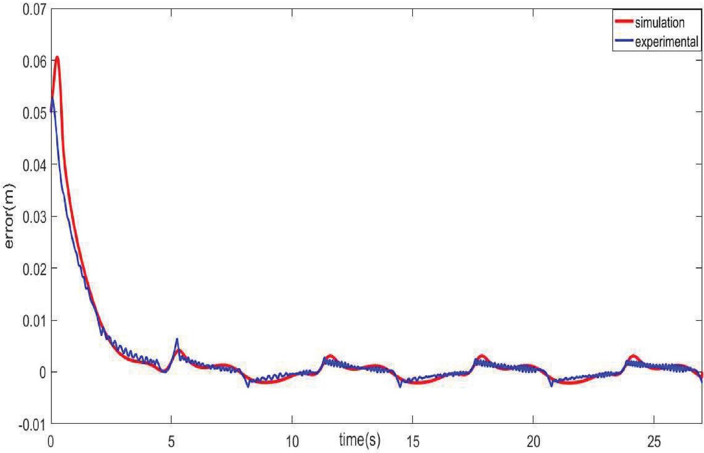
Figure 15(c): Experimental and simulation trajectory tracking error of (DAFNN) controller with the weight parameters tuning for tracking case (1).

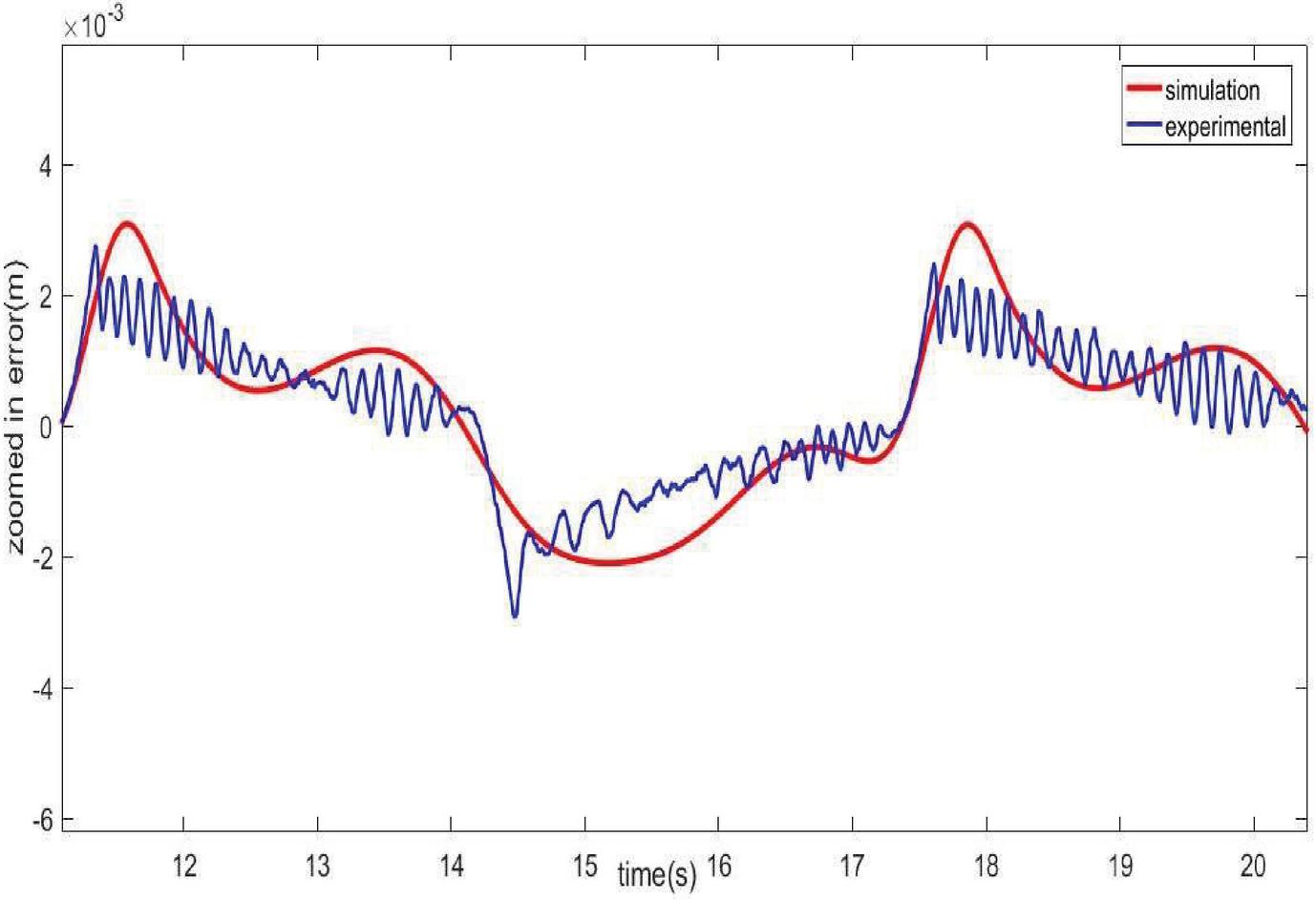
Figure 15(d): Experimental and simulation zoomed in trajectory tracking error of (DAFNN) controller with the weight parameters tuning for tracking case (1).

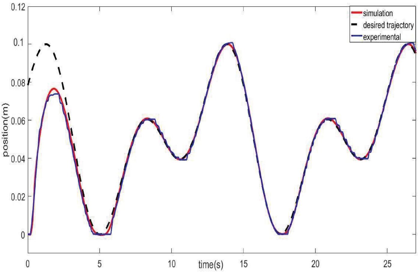
Figure 16(a): Experimental output and simulation output of (DAFNN) controller with the weight parameters tuning for tracking case (2).

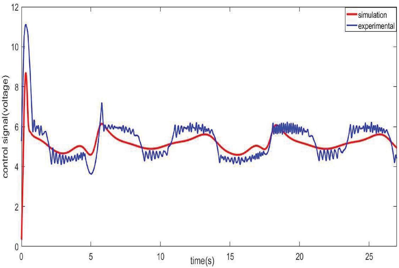
Figure 16(b): Experimental system and simulation control signal of (DAFNN) controller with the weight parameters tuning for tracking case (2).

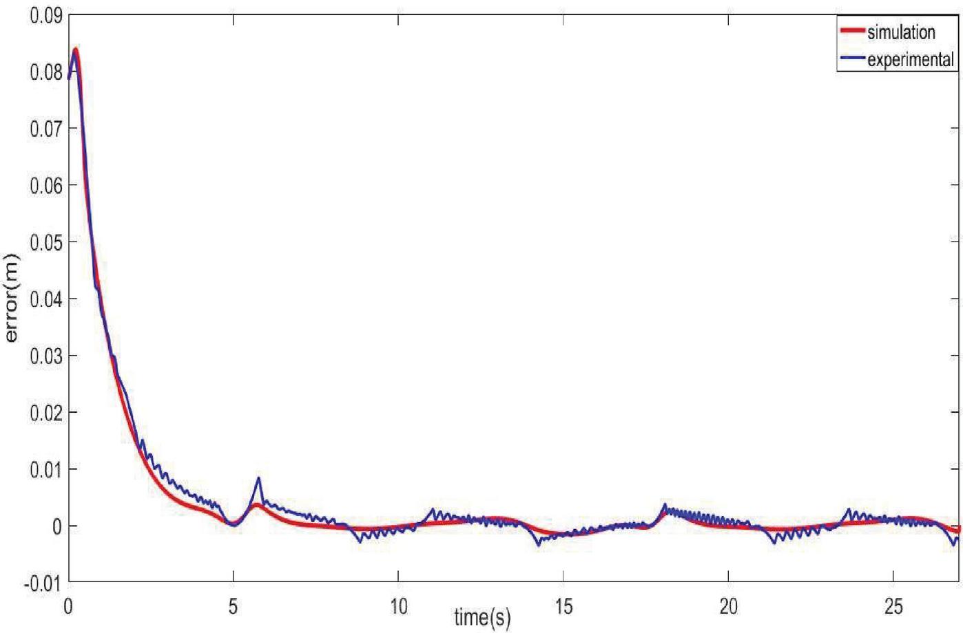
Figure 16(c): Experimental and simulation trajectory tracking error of (DAFNN) controller with the weight parameters for tracking case (2).

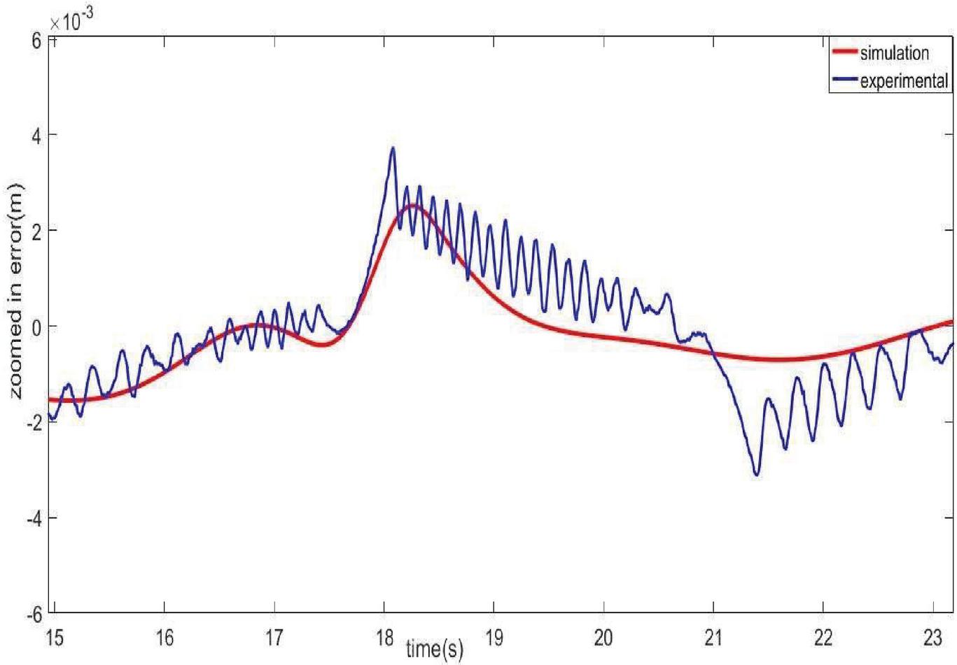
Figure 16(d): Experimental and simulation zoomed in trajectory tracking error of (DAFNN) controller with the weight parameters for tracking case (2).

By comparing the results for both methods, it is obvious that the hybrid tuning method has a significant effect on the DAFN controller tracking error reduction.

To measure the performance of the controller for tracking the desired trajectories, the root square mean error (RSME) performance assessment criteria obtained as below is investigated.

$$RSME=\sqrt{\frac{1}{n}{\int }_{i=1}^n{(y_d{}_i-x_i)}^2}$$

(66)

Where $n$ implies the number of samples.

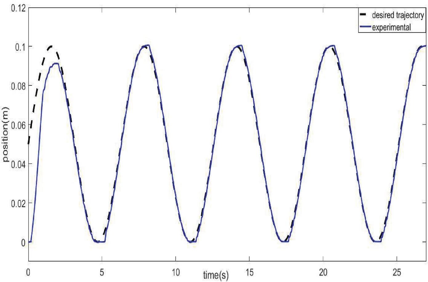
Figure 17(a): Experimental output and desired trajectory of (DAFNN) controller with hybrid tuning for tracking case (1) when $M=18$ kg $\to$ 3 kg.

The non-identical initial conditions between the output and the desire’s values, result in an uncontrollable error, hence, to evaluate the performance precisely, the RSME can be calculated when the two values reach each other. The RSME for hybrid and weight tuning method tracking sinusoidal is calculated $0.9$ and $1.4$, respectively.

4.1.1 Discussion

In Table 1, the performance of the proposed controller tracking the sine trajectories for frequency 0.1, is compared with the references (Najafi et al., 2009; Nazari and Surgenor, 2016) and (H. K. Lee et al., 2002). An efficient comparison requires that the environmental conditions, components of the pneumatic system (cylinder, valve and payload), operation condition (amplitude, initialization, supply pressure) and accuracy of the sensors used for experiments are similar. Therefore, it is vital to consider these factors to compare the performance of controllers properly under different conditions. As it is shown in Table 1, (Najafi et al., 2009) have been obtained the best performance and our proposed (DAFNN controller with hybrid tuning) work is the second best based RSME comparison. However, our proposed controller performs the best MAE compared to other works. Although the performance of controller with weight tuning has dropped, for both criteria it has shown better performance compared to (H. K. Lee et al., 2002).

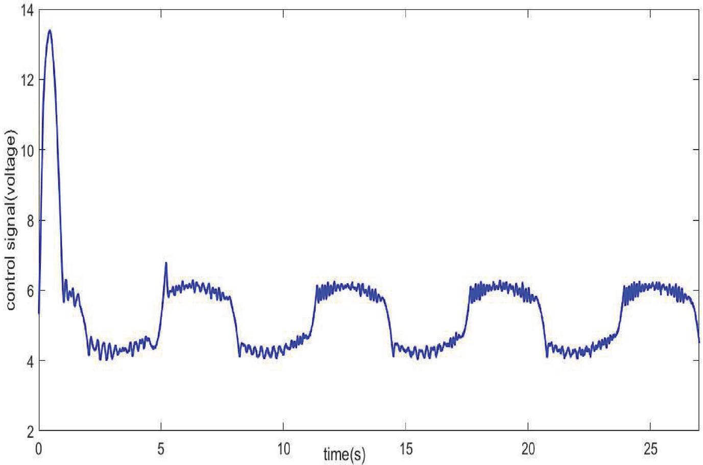
Figure 17(b): Experimental system control signal of (DAFNN) controller with hybrid tuning for tracking case (1) when $M=18$ kg $\to$ 3 kg.

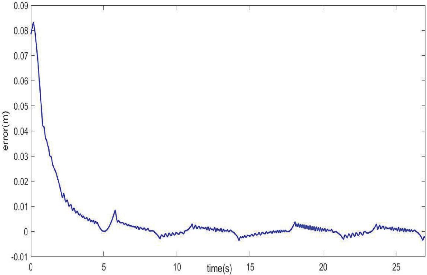
Figure 17(c): Experimental trajectory tracking error of (DAFNN) controller with hybrid tuning for tracking case (1) when $M=18$ kg $\to$ 3 kg.

Figure 17(d): Experimental zoomed in trajectory tracking error of (DAFNN) controller with hybrid tuning for tracking case (1) $M=18$ kg $\to$ 3 kg.

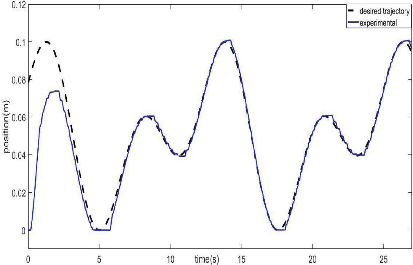
Figure 18(a): Experimental output and desired trajectory of (DAFNN) controller with hybrid tuning for tracking case (2) when $M=18$ kg $\to$ 3 kg.

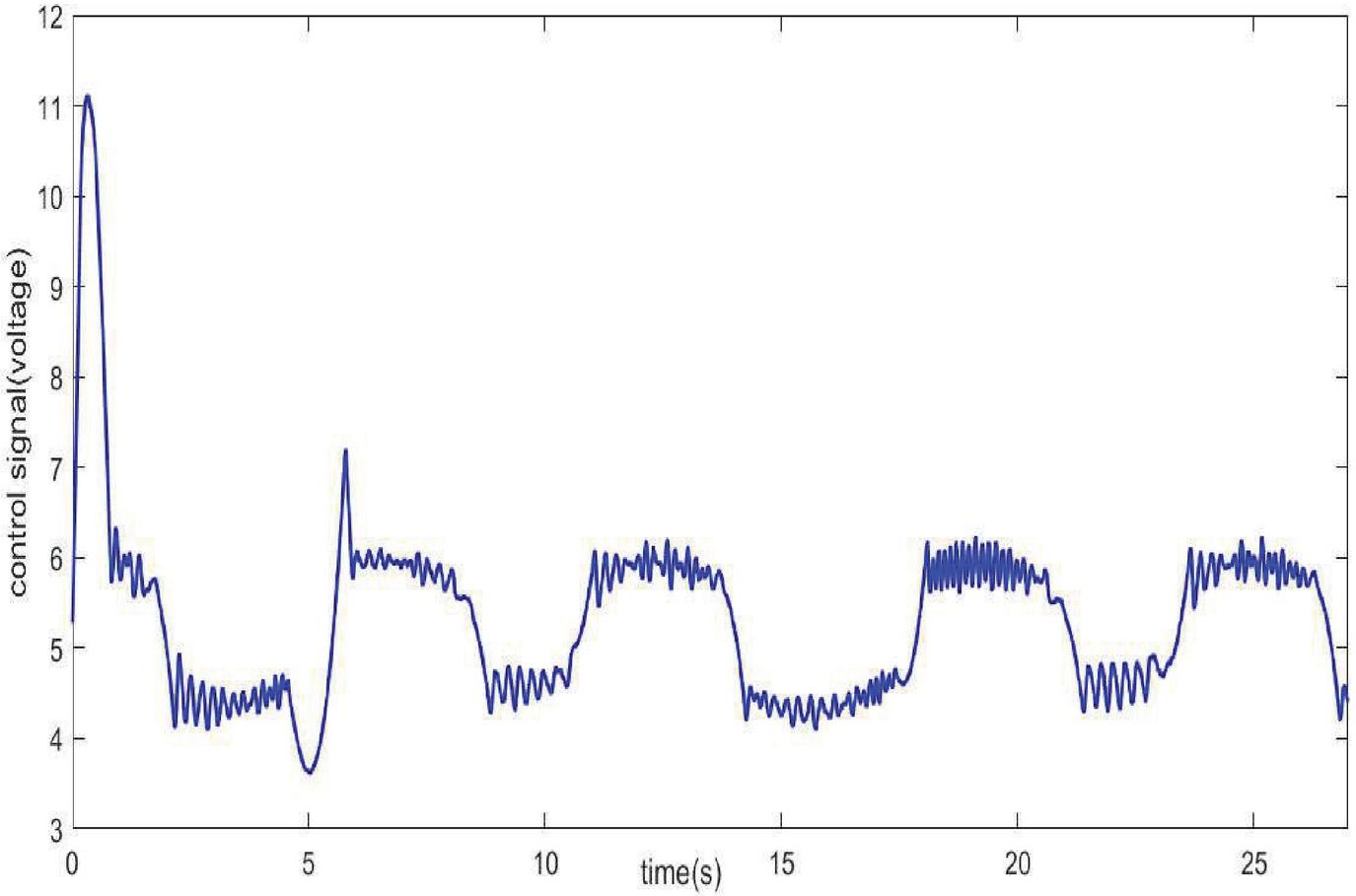
Figure 18(b): Experimental system control signal of (DAFNN) controller with hybrid tuning for tracking case (2) when $M=18$ kg $\to$ 3 kg.

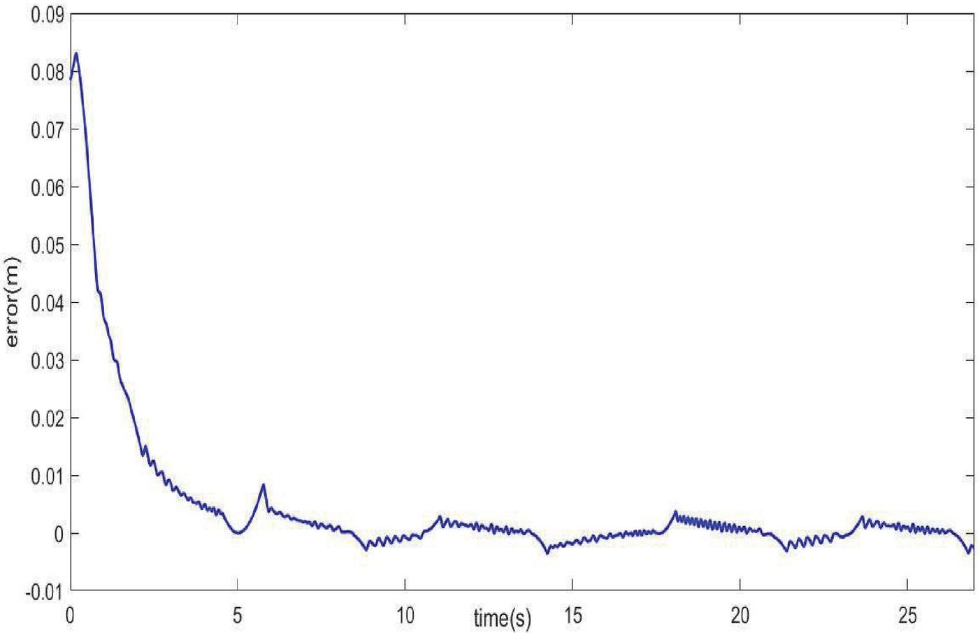
Figure 18(c): Experimental trajectory tracking error of (DAFNN) controller with hybrid tuning for tracking case (2) $M=18$ kg $\to$ 3 kg.

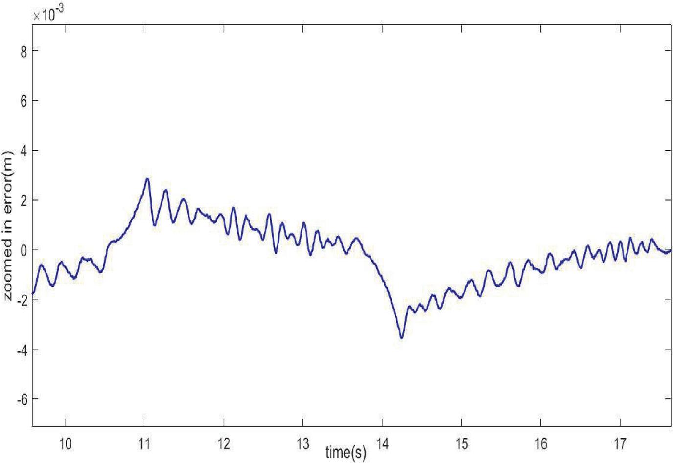
Figure 18(d): Experimental zoomed in trajectory tracking error of (DAFNN) controller with hybrid tuning for tracking case (2) $M=18$ kg $\to$ 3 kg.

4.2 Robustness Tests Against Mass Load Variation

The better the controller adapts to the new conditions, the more robust it will be. On the other word, the control approach sensitivity, when nominal parameters of the system change could index whether the control is robust or not. To investigate the control resistance, in the first test, the controller is conducted based on a nominal mass load of 18 kg. Afterwards, exploiting the adaptive property, it is expected that the control strategy could adapt to a new and non-nominal mass load of 3kg. In Figures 17 and 18, the results of the practical control system are illustrated when the load is changed from 18 to 3 kg. As presented in Figures 17(d) and 18(d), the tracking error for desired trajectory case (1) and case (2) is $\pm$3 mm and $\pm$3mm respectively. The results show that the (DAFNN) controller is robust when payload changes in practical system.

5 Conclusion

In this paper, a Neural Network (NN) system for modelling and a Fuzzy Neural (NN) for control the nonlinear pneumatic actuator system are used. Using the neural network advantages it does not require modelling of complex terms such as mass flow in proportional valve and friction force, and an accurate identification are established for practical pneumatic servo system.

For trajectory tracking control purpose, a direct adaptive fuzzy neural network (DAFNN) controller is designed. The Fuzzy logic system used in this paper has some differences in rule base with a traditional system. In the presence of uncertainty and unknown dynamics, the proposed controller tracks the desired trajectories successfully, as well as the controller is robust against payload variation. A novel comparison for adjustment methods of control parameters is accomplished. Finally, results are Utilizing Lyapunov theory, close-loop system stability and boundedness of parameters are proved.

Disclosure Statement:

No potential conflict of interest was reported by the authors.

Funding:

Not applicable.

References

Ahn, K. K., and Anh, H. P. H. (2009). Design and implementation of an adaptive recurrent neural networks (ARNN) controller of the pneumatic artificial muscle (PAM) manipulator. Mechatronics, 19(6), pp. 816–828.

Al-Saloum, S., Taha, A., and Chouaib, I. (2017). Parameter identification of a jet pipe electro-pneumatic servo actuator. International Journal of Fluid Power, 18(1), pp. 49–69.

Bone, G. M., and Ning, S. (2007). Experimental comparison of position tracking control algorithms for pneumatic cylinder actuators. IEEE/ASME Transactions on mechatronics, 12(5), pp. 557–561.

Bounemeur, A., Chemachema, M., and Essounbouli, N. (2018). Indirect adaptive fuzzy fault-tolerant tracking control for MIMO nonlinear systems with actuator and sensor failures. ISA transactions, 79, pp. 45–61.

Carneiro, J. F., and de Almeida, F. G. (2012). A neural network based nonlinear model of a servopneumatic system. Journal of Dynamic Systems, Measurement, and Control, 134(2), p. 024502.

Chen, S.-Y., and Gong, S.-S. (2017). Speed tracking control of pneumatic motor servo systems using observation-based adaptive dynamic sliding-mode control. Mechanical Systems and Signal Processing, 94, pp. 111–128.

Chen, S., Wang, X., and Harris, C. J. (2007). NARX-based nonlinear system identification using orthogonal least squares basis hunting. IEEE Transactions on Control Systems Technology, 16(1), pp. 78–84.

Gao, Q., Feng, G., Wang, Y., and Qiu, J. (2012). Universal fuzzy models and universal fuzzy controllers for stochastic nonaffine nonlinear systems. IEEE Transactions on Fuzzy systems, 21(2), pp. 328–341.

Gao, X., and Feng, Z.-J. (2005). Design study of an adaptive Fuzzy-PD controller for pneumatic servo system. Control Engineering Practice, 13(1), pp. 55–65.

Hajji, S., Ayadi, A., Smaoui, M., Maatoug, T., Farza, M., and M’saad, M. (2019). Position control of pneumatic system using high gain and backstepping controllers. Journal of Dynamic Systems, Measurement, and Control, 141(8), p. 081001.

Han, H.-G., Wu, X.-L., Liu, Z., and Qiao, J.-F. (2017). Design of Self-Organizing Intelligent Controller Using Fuzzy Neural Network. IEEE Transactions on Fuzzy systems, 26(5), pp. 3097–3111.

Kaitwanidvilai, S., and Parnichkun, M. (2005). Force control in a pneumatic system using hybrid adaptive neuro-fuzzy model reference control. Mechatronics, 15(1), pp. 23–41.

Kasabov, N. K., and Song, Q. (2002). DENFIS: dynamic evolving neural-fuzzy inference system and its application for time-series prediction. IEEE Transactions on Fuzzy systems, 10(2), pp. 144–154.

Khalil, H. K. (2002). Nonlinear systems. Upper Saddle River.

Laghrouche¶, S., Smaoui, M., Plestan, F., and Brun, X. (2006). Higher order sliding mode control based on optimal approach of an electropneumatic actuator. International journal of Control, 79(2), pp. 119–131.

Lai, Y.-Y., and Chang, K.-M. (2017). Fuzzy control for a pneumatic positioning system. 2017 9th International Conference on Modelling, Identification and Control (ICMIC).

Lee, H. K., Choi, G. S., and Choi, G. H. (2002). A study on tracking position control of pneumatic actuators. Mechatronics, 12(6), pp. 813–831.

Lee, L.-W., and Li, I.-H. (2016). Design and implementation of a robust FNN-based adaptive sliding-mode controller for pneumatic actuator systems. Journal of Mechanical Science and Technology, 30(1), pp. 381–396.

Leng, G., Prasad, G., and McGinnity, T. M. (2004). An on-line algorithm for creating self-organizing fuzzy neural networks. Neural Networks, 17(10), pp. 1477–1493.

Lin, F.-J., and Wai, R.-J. (2001). Hybrid control using recurrent fuzzy neural network for linear induction motor servo drive. IEEE Transactions on Fuzzy systems, 9(1), pp. 102–115.

Liu, Y.-T., Kung, T.-T., Chang, K.-M., and Chen, S.-Y. (2013). Observer-based adaptive sliding mode control for pneumatic servo system. Precision Engineering, 37(3), pp. 522–530.

Maré, J.-C., Geider, O., and Colin, S. (2000). An improved dynamic model of pneumatic actuators. International Journal of Fluid Power, 1(2), pp. 39–49.

Najafi, F., Fathi, M., and Saadat, M. (2009). Performance improvement of a PWM-sliding mode position controller used in pneumatic actuation. Intelligent Automation and Soft Computing, 15(1), pp. 73–84.

Nazari, V., and Surgenor, B. (2016). Improved position tracking performance of a pneumatic actuator using a fuzzy logic controller with velocity, system lag and friction compensation. International Journal of Control, Automation and Systems, 14(5), pp. 1376–1388.

Neji, Z., and Beji, F.-M. (2000). Neural Network and time series identification and prediction. Proceedings of the IEEE-INNS-ENNS International Joint Conference on Neural Networks. IJCNN 2000. Neural Computing: New Challenges and Perspectives for the New Millennium.

Ning, S., and Bone, G. M. (2005). Development of a nonlinear dynamic model for a servo pneumatic positioning system. IEEE International Conference Mechatronics and Automation, 2005.

Osman, K., Rahmat, M., Azman, M. A., and Suzumori, K. (2012). System identification model for an Intelligent Pneumatic Actuator (IPA) system. 2012 IEEE/RSJ International Conference on Intelligent Robots and Systems.

Park, J.-H., Huh, S.-H., Kim, S.-H., Seo, S.-J., and Park, G.-T. (2005). Direct adaptive controller for nonaffine nonlinear systems using self-structuring neural networks. IEEE Transactions on neural networks, 16(2), pp. 414–422.

Phan, P. A., and Gale, T. J. (2008). Direct adaptive fuzzy control with a self-structuring algorithm. Fuzzy Sets and Systems, 159(8), pp. 871–899.

Smaoui, M., Brun, X., and Thomasset, D. (2006). A study on tracking position control of an electropneumatic system using backstepping design. Control Engineering Practice, 14(8), pp. 923–933.

Sun, G., Wang, D., Peng, Z., Wang, H., Lan, W., and Wang, M. (2013). Robust adaptive neural control of uncertain pure-feedback nonlinear systems. International journal of Control, 86(5), pp. 912–922.

Theodoridis, D., Boutalis, Y., and Christodoulou, M. (2012). Direct adaptive neuro-fuzzy trajectory tracking of uncertain nonlinear systems. International Journal of Adaptive Control and Signal Processing, 26(7), pp. 660–688.

Tsai, Y.-C., and Huang, A.-C. (2008). Multiple-surface sliding controller design for pneumatic servo systems. Mechatronics, 18(9), pp. 506–512.

Zhu, Y., and Barth, E. J. (2010). Accurate sub-millimeter servo-pneumatic tracking using model reference adaptive control (MRAC). International Journal of Fluid Power, 11(2), pp. 43–55.

Biographies

Peyman Mawlani held a bachelor of science degree in mechanical engineering from the University of Tabriz, Iran in 2016. Afterward, he attended the Shahid Rajaee Teacher Training University, Iran where he received his M.Sc. in Mechanical Engineering in 2019. His research interest is control design for non-linear systems and robotic, as well as applying machine learning and artificial intelligent application in robotics.

Mohammadreza Arbabtafti received a B.S. degree in Mechanical Engineering in 2002 from Isfahan University of Technology, Iran. He received his M.S. and Ph.D. degrees in Mechanical Engineering in 2004 and 2010 from Tarbiat Modares University, Iran. He is a recipient of Khwarizmi Young Award 2008. He is currently on the faculty of Shahid Rajaee Teacher Training Univeristy in Iran. His research interest is in the area of haptics and robotics.

International Journal of Fluid Power, Vol. 21_1, 1–44.
doi: 10.13052/ijfp1439-9776.2211
© 2021 River Publishers

Abstract

1 Introduction

2 Modelling and System Description

2.1 System Hardware and Software

2.2 Modelling and Identification

2.3 Neural Network Model Validation

3 Controller Design and Stability Analysis

3.1 Problem Statement

3.2 Feedback Linearization

3.3 Direct Adaptive Fuzzy Neural Network (DAFNN) Control Design

4 Simulation and Experimental Results

4.1 Trajectory Tracking Control

4.1.1 Discussion

4.2 Robustness Tests Against Mass Load Variation

5 Conclusion

Disclosure Statement:

Funding:

References

Biographies