Research on Compliant Controller of Underwater Mechanical Capture System Based on Impedance Theory

Yuanjie Liu¹, Fusheng Zha^1,*, Qiming Wang¹, Chao Zheng², Jinrui Zhou¹ and Lianzhao Zhang¹

¹State Key Laboratory of Robotics and System, Harbin institute of Technology, Harbin, China
²Wuhan Second Ship Design and Research Institute, Wuhan, China
E-mail: zhafusheng@hit.edu.cn
*Corresponding Author

Received 30 March 2022; Accepted 09 June 2022; Publication 12 June 2023

Abstract

Due to the requirement of the exploitation of marine resources, the execution of specific underwater tasks by onboard manipulators has become one of the key research fields in domestic and all over the world. Based on the underwater capture system designed for the UUV recycling task, which consists of an underwater manipulator and a mechanical capture device, this paper first constructs the kinematics and dynamics model of the capture system through theoretical analysis such as theoretical mechanics and theory of mechanism. Then, combined with the requirements of the recycling task, through the theoretical basis of fluid mechanics such as Morrison equation, dynamic of the capture system in underwater environment is analysed, with a compliant controller designed for the capture system based on impedance theory in order to reduce the impact of underwater environment in the capture task. Moreover, as the capture system modelled in the Adams dynamics simulation platform, it is verified that the designed compliant controller can reduce the underwater environmental impact through simulation experiments in the Adams dynamic platform.

Keywords: Compliant controller, underwater manipulator, hydraulic analysis, dynamics simulation.

1 Introduction

With the gradual reduction of land resources, the degree of development and utilization of marine resources has gradually become one of the standards for measuring the power of science and technology for a country [1]. In recent years, with the development of technology in related fields such as robotics, it has gradually become possible to carry out special underwater tasks by carrying specific actuators on onboard manipulators [2–4].

Unmanned underwater vehicle (UUV) has the characteristics of wide working space and strong cruising ability in underwater environment, which plays an irreplaceable role in underwater exploration, underwater positioning and deep-sea sampling. Due to the limited energy carried by the UUV, it is necessary to release and recycle the UUV at the beginning and end of the exploration. Thus, utilizing the mechanical operation system of the onboard manipulator to carry the mechanical capture device, as well as building a manipulator controller suitable for the underwater environment are indispensable parts in the close loop of underwater exploration task [5].

Different from conventional industrial manipulators, the study of underwater manipulator must fully analyse the complex marine environment, whose working accuracy is affected by factors such as fluid viscosity resistance and ocean current impact [6]. However, dynamic underwater environmental factors such as ocean current impact and undercurrent not only have a high degree of uncertainty that is difficult to predict and model, but also, in general, generate larger force and faster mutation to the manipulator, compared with static environmental forces such as viscous resistance and buoyancy, leading to the existence of a lot of uncertain parameters in the dynamic modelling of the manipulator [7]. Since Morison equation was proposed to calculate the wave loads on cylindrical components in the ocean, it has been widely applied on the calculation of hydrodynamic terms for underwater manipulator. Since the motion of the manipulator is severely affected by the flow around the manipulator which cause complex fluid-structure interaction, there is no better calculation method to replace Morison equation in the calculation of the hydrodynamic resistance of the manipulator.

In 1984 Hogan [8] proposed impedance control theory, the basic idea of which is adjusting the manipulators’ stiffness in order to maintain ideal dynamic character during interaction with environment. Till now, many scholars have done much research on force and displacement control strategy in time-varying and stochastic environments using impedance control methods. Sheng et al. (2018) designed a fuzzy adaptive hybrid impedance control scheme for the support side of a mirror milling system to solve the support problem with time-varying environmental stiffness [9]. Kang et al. (2020) proposed a variable target stiffness adaptive impedance control method for wheel-legged robots on complex unknown terrain [10]. Liang et al. (2021) proposed an impedance control method for handling unpredictable and time-varying adhesion forces for a rubber depalletizing robot [11].

Currently, most of the control methods for manipulator to cope with variable loads underwater are implemented with adaptive control methods. For example, Carlucho et al. designed an adaptive controller for variable payloads in underwater environment [12], which was implemented with the help of MPC method with data-driven techniques. However, as it stands, the problem that the data-driven approach cannot ensure the control requirements may arise in case of the fluctuation of the systematic dynamic factors.

As for the marine environment in real world, it is difficult to develop a stable current environment, which in another word is mostly turbulent. As a result, it is difficult to eliminate the influence of the underwater dynamic environmental constraint force on the entire manipulator system and the impact caused by the contact between the end effector and the UUV only by the position servo controller, since it is easy to cause damage to the mechanical structure of the manipulator. Therefore, it is necessary to establish a compliant controller for the underwater capture system, in order to avoid mechanical structure damage by compensating the contact force among the manipulator and the environment, as well as the UUV. In this paper, in the beginning, based on the mechanism characteristics of the manipulator, the forward and inverse kinematic solution equations of the manipulator are established. In addition, the kinetic equations are combined with Morrison’s equation to establish the manipulator dynamic model under turbulent flow conditions. Moreover, based on the impedance control theory, a complaint control strategy is proposed to avoid structural damage of the manipulator under the influence of uncertain wave loads by adding virtual impedance. At last, based on the structural characteristics of the manipulator, a detailed structural model of the manipulator is built, and the effectiveness of the impedance control strategy in presenting resistance to water flow disturbance is fully verified by simulating the turbulence phenomenon in the simulation platform and applying the proposed complaint control strategy to the structural model of the manipulator in the platform.

Nomenclature

$i$	Joint number
$X_i$, $Y_i$, $Z_i$	Joint coordinate based on the D-H method
$a_i$	Length of the link, represents the distance from axis $Z_{i-1}$ to axis $Z_i$ along axis
${\alpha }_i$	Torsion angle of the link, represents the angle rotating from axis $Z_{i-1}$ to axis $Z_i$ around axis $X_i$
$d_i$	Offset of the link, represents the distance from axis $X_{i-1}$ to axis $X_i$ along axis $Z_{i-1}$
${\theta }_i$	Rotation angle of the link, represents angle rotating from axis $X_{i-1}$ to axis $X_i$ around axis $Z_{i-1}$
${}_i{}^{i-1}T$	Linkage transformation matrix
$c_i$	$\cos {\theta }_i$
$s_i$	$\sin {\theta }_i$
$s_{ij}$	$\sin ({\theta }_i+{\theta }_j)$
$c_{ij}$	$\cos ({\theta }_i+{\theta }_j)$
$\tau$	Driving torque of the manipulator’s joint
${\tau }_h$	Hydrodynamic term of the manipulator
$\dot{\theta }$	Angular velocity of the manipulator’s joint
$\ddot{\theta }$	Angular acceleration of the manipulator’s joint
$M(\theta )$	Third-order positive definite inertia matrix of the mass
$C(\theta ,\dot{\theta })$	The centrifugal force and the Coriolis force vector
$H(\theta )$	Equivalent gravity term
$g$	Gravitational acceleration
$\rho$	Density of the water
${\rho }_m$	Density of the manipulator
$m_i$	Equivalent mass of link $i$
$F$	Acting force per unit length along the manipulator
$F_d$	Hydrodynamic resistance per unit length along the manipulator
$F_m$	Inertial force (additional mass force) per unit length along the manipulator
$A$	Projected area of the manipulator’s link in the direction perpendicular to the incoming flow velocity
$v(x)$	Velocity function
$C_m$	Additional mass coefficient
$C_d$	Hydrodynamic resistance coefficient
$D$	Diameter of the cylinder joint
$\mathrm{d}l$	Thickness of the cylinder element
${\tau }_{\mathrm{D}i}$	Hydrodynamic resistance moment of the Joint $i$
${\tau }_{\mathrm{A}i}$	Additional mass moment of the Joint $i$
$v_{i-j}^n$	Normal velocity of linkage $i$ due to joint $j$ motion over the length of the unit
$M_d$	Designed inertia matrix
$B_d$	Designed damping matrix
$K_d$	Designed stiffness matrix
$X_e,{\dot{X}}_e,{\ddot{X}}_e$	Actual position, actual velocity, and actual acceleration of the end of the manipulator
$X_d,{\dot{X}}_d,{\ddot{X}}_d$	Designed position, designed speed, and designed acceleration of the end of the manipulator
$F_d$	Expected contact force
$F_e$	Actual contact force
${\tau }_w$	Hydrodynamic force of each joint in the dynamic water environment

2 Establishment of the Kinematics and Dynamics Model of the Capture System

2.1 Kinematics Model of the Capture System

This study uses the D-H method to establish the kinematic model of the underwater manipulator, mainly to obtain the linear mapping relationship of the robot’s position, velocity, and acceleration in the joint space and the drive space, and obtain the schematic diagram, displaying the joint coordinates distribution of the underwater manipulator, as is shown in Figure 1.

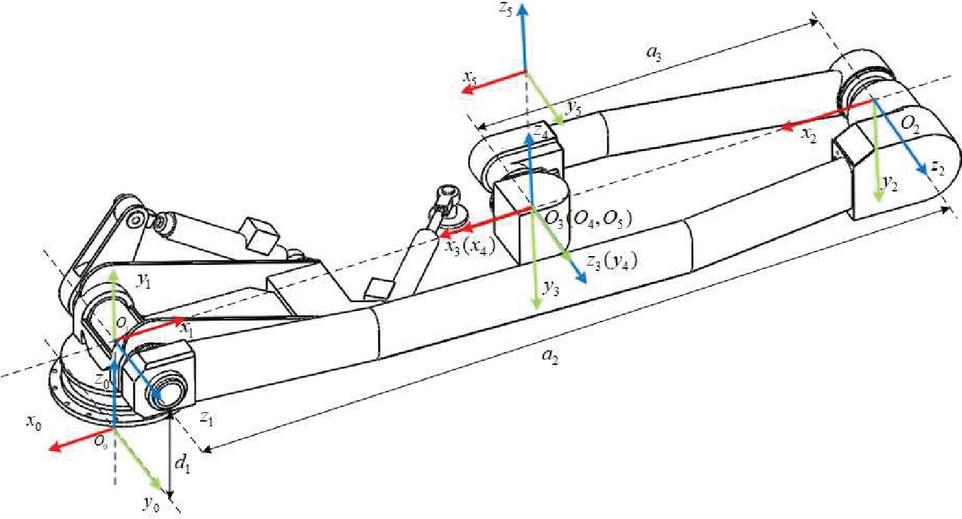
Figure 1 Connecting rod coordinate system.

In order to study the kinematics of the manipulator, the model of the manipulator is simplified to a link model by the D-H method. Table 1 shows the parameters of the D-H link obtained according to the joint coordinate system, in which the length of the link $a_i$ represents the distance from axis $Z_{i-1}$ to axis $Z_i$ along axis $X_i$, the torsion angle of the link ${\alpha }_i$ represents the angle rotating from axis $Z_{i-1}$ to axis $Z_i$ around axis $X_i$, the offset of the link $d_i$ represents the distance from axis $X_{i-1}$ to axis $X_i$ along axis $Z_{i-1}$, and the rotation angle of the link ${\theta }_i$ represents angle rotating from axis $X_{i-1}$ to axis $X_i$ around axis $Z_{i-1}$.

Table 1 D-H parameter table of underwater manipular

Joint $i$	$a_i$/m	${\alpha }_i$/(${}^{\circ }$)	$d_i$/m	${\theta }_i$/(${}^{\circ }$)
1	0	90	$d_1$	${\theta }_1$
2	$a_2$	0	0	${\theta }_2$
3	$a_3$	0	0	${\theta }_3$
4	0	90	0	${\theta }_4$
5	0	0	0	${\theta }_5$

According to the established coordinate system of the manipulator and the D-H parameters in Table 1, the kinematics equation can be directly established through the coordinate transformation matrix. The general expression of the transformation matrix between two adjacent links is shown in Equation (1):

$${}_i{}^{i-1}T=\left[\begin{array}{cccc}\hfill \cos {\theta }_i\hfill & \hfill -\cos {\alpha }_i\sin {\theta }_i\hfill & \hfill \sin {\alpha }_i\sin {\theta }_i\hfill & \hfill a_i\cos {\theta }_i\hfill \\ \hfill \sin {\theta }_i\hfill & \hfill \cos {\alpha }_i\cos {\theta }_i\hfill & \hfill -\sin {\alpha }_i\cos {\theta }_i\hfill & \hfill a_i\sin \theta \hfill \\ \hfill 0\hfill & \hfill \sin {\alpha }_i\hfill & \hfill \cos {\alpha }_i\hfill & \hfill d_i\hfill \\ \hfill 0\hfill & \hfill 0\hfill & \hfill 0\hfill & \hfill 1\hfill \end{array}\right]$$

(1)

Substitute the D-H parameters in Table 1 into Equation (1), the transformation matrix of each link can be obtained, the results of which are shown in Equations (2)–(6)

$${}_1{}^{0}T=\left[\begin{array}{cccc}\hfill \cos {\theta }_1\hfill & \hfill 0\hfill & \hfill \sin {\theta }_1\hfill & \hfill 0\hfill \\ \hfill \sin {\theta }_1\hfill & \hfill 0\hfill & \hfill -\cos {\theta }_1\hfill & \hfill 0\hfill \\ \hfill 0\hfill & \hfill 1\hfill & \hfill 0\hfill & \hfill d_1\hfill \\ \hfill 0\hfill & \hfill 0\hfill & \hfill 0\hfill & \hfill 1\hfill \end{array}\right]$$	(2)
$${}_2{}^{1}T=\left[\begin{array}{cccc}\hfill \cos {\theta }_2\hfill & \hfill -\sin {\theta }_2\hfill & \hfill 0\hfill & \hfill a_2\cos {\theta }_2\hfill \\ \hfill \sin {\theta }_2\hfill & \hfill \cos {\theta }_2\hfill & \hfill 0\hfill & \hfill a_2\sin {\theta }_2\hfill \\ \hfill 0\hfill & \hfill 0\hfill & \hfill 1\hfill & \hfill 0\hfill \\ \hfill 0\hfill & \hfill 0\hfill & \hfill 0\hfill & \hfill 1\hfill \end{array}\right]$$	(3)
$${}_3{}^{2}T=\left[\begin{array}{cccc}\hfill \cos {\theta }_3\hfill & \hfill -\sin {\theta }_3\hfill & \hfill 0\hfill & \hfill a_3\cos {\theta }_3\hfill \\ \hfill \sin {\theta }_3\hfill & \hfill \cos {\theta }_3\hfill & \hfill 0\hfill & \hfill a_3\sin {\theta }_3\hfill \\ \hfill 0\hfill & \hfill 0\hfill & \hfill 1\hfill & \hfill 0\hfill \\ \hfill 0\hfill & \hfill 0\hfill & \hfill 0\hfill & \hfill 1\hfill \end{array}\right]$$	(4)
$${}_4{}^{3}T=\left[\begin{array}{cccc}\hfill \cos {\theta }_4\hfill & \hfill 0\hfill & \hfill \sin {\theta }_4\hfill & \hfill 0\hfill \\ \hfill \sin {\theta }_4\hfill & \hfill 0\hfill & \hfill -\cos {\theta }_4\hfill & \hfill 0\hfill \\ \hfill 0\hfill & \hfill 1\hfill & \hfill 0\hfill & \hfill 0\hfill \\ \hfill 0\hfill & \hfill 0\hfill & \hfill 0\hfill & \hfill 1\hfill \end{array}\right]$$	(5)
$${}_5{}^{4}T=\left[\begin{array}{cccc}\hfill \cos {\theta }_5\hfill & \hfill -\sin {\theta }_5\hfill & \hfill 0\hfill & \hfill 0\hfill \\ \hfill \sin {\theta }_5\hfill & \hfill \cos {\theta }_5\hfill & \hfill 0\hfill & \hfill 0\hfill \\ \hfill 0\hfill & \hfill 0\hfill & \hfill 1\hfill & \hfill 0\hfill \\ \hfill 0\hfill & \hfill 0\hfill & \hfill 0\hfill & \hfill 1\hfill \end{array}\right]$$	(6)

For a manipulator with five degrees of freedom, the transformation matrix from the base coordinate system to the ending joint coordinate system is shown in Equation (7)

$${}_5{}^{0}T={}_1{}^{0}T{}_2{}^{1}T{}_3{}^{2}T{}_4{}^{3}T{}_5{}^{4}T$$

(7)

Substituting Equations (2) to (6) into Equation (7), Equation (8) can be required:

$${}_5{}^{0}T=\left[\begin{array}{cccc}\hfill r_{11}\hfill & \hfill r_{12}\hfill & \hfill r_{13}\hfill & \hfill p_x\hfill \\ \hfill r_{21}\hfill & \hfill r_{22}\hfill & \hfill r_{23}\hfill & \hfill p_y\hfill \\ \hfill r_{31}\hfill & \hfill r_{32}\hfill & \hfill r_{33}\hfill & \hfill p_z\hfill \\ \hfill 0\hfill & \hfill 0\hfill & \hfill 0\hfill & \hfill 1\hfill \end{array}\right]$$

(8)

The value of each element in Equation (8) is

$$\{\begin{array}{c}{r}_{11}=s_1{s}_5+c_1{c}_5{c}_{234},r_{12}=s_1{c}_5-c_1{s}_5{c}_{234}\hfill \\ r_{13}=c_1{s}_{234},r_{21}=s_1{c}_5{c}_{234}-c_1{s}_5\hfill \\ r_{22}=-c_1{c}_5-s_1{s}_5{c}_{234},r_{23}=s_1{s}_{234}\hfill \\ r_{31}=c_5{s}_{234},r_{32}=-s_5{s}_{234},r_{33}=-c_{234}\hfill \\ p_x=a_2{c}_1{c}_2+a_3{c}_1{c}_{23}\hfill \\ p_y=a_2{s}_1{c}_2+a_3{s}_1{c}_{23}\hfill \\ p_z=d_1+a_2{s}_2+a_3{s}_{23}\hfill \end{array}$$

(9)

In which, $c_i=\cos {\theta }_i,s_i=\sin {\theta }_i,s_{ij}=\sin ({\theta }_i+{\theta }_j),c_{ij}=\cos ({\theta }_i+{\theta }_j)$.

The inverse kinematics analysis of the manipulator is to solve the rotation of each joint of the manipulator by analyzing the position and posture of capture device at the end of the manipulator. When the value in the transformation matrix ${}_5{}^{0}T$ is known, Equation (2.1) can be solved by Equation (9).

${}_5{}^{0}T$	$=\left[\begin{array}{cccc}\hfill r_{11}\hfill & \hfill r_{12}\hfill & \hfill r_{13}\hfill & \hfill p_x\hfill \\ \hfill r_{21}\hfill & \hfill r_{22}\hfill & \hfill r_{23}\hfill & \hfill p_y\hfill \\ \hfill r_{31}\hfill & \hfill r_{32}\hfill & \hfill r_{33}\hfill & \hfill p_z\hfill \\ \hfill 0\hfill & \hfill 0\hfill & \hfill 0\hfill & \hfill 1\hfill \end{array}\right]$
	$={}_1{}^{0}T({\theta }_1){}_2{}^{1}T({\theta }_2){}_3{}^{2}T({\theta }_3){}_4{}^{3}T({\theta }_4){}_5{}^{4}T({\theta }_5)$	(10)

Solving the position angle of each joint ${\theta }_i$, it can be required as follow:

$$\{\begin{array}{c}{\theta }_1=\mathrm{atan2}(p_y,p_x)\hfill \\ {\theta }_2=\mathrm{atan2}(p_z-d_1,\pm \sqrt{{\gamma }^2-{(p_z-d_1)}^2})-\mathrm{atan2}(a_3{s}_3,a_3{c}_3+a_2)\hfill \\ {\theta }_3=\mathrm{atan2}(\pm \sqrt{4a_2^2{a}_3^2-K^2},K)\hfill \\ {\theta }_4=\mathrm{atan2}(r_{33}{s}_{23}+r_{13}{c}_1{c}_{23}+r_{23}{c}_{23}{s}_1,\hfill \\ -r_{33}{c}_{23}+r_{13}{c}_1{s}_{23}+r_{23}{s}_{23}{s}_1)\hfill \\ {\theta }_5=\mathrm{atan2}(r_{21}{c}_1-r_{11}{s}_1,r_{22}{c}_1-r_{12}{s}_1)\hfill \end{array}$$

In which, $K=p_x^2+p_y^2+{(p_z-d_1)}^2-a_2^2-a_3^2$.

2.2 Dynamic Analysis of the Manipulator of the Capture System

Since the influence to the dynamic of the entire system of the rotation of the joint on manipulator’s wrist is relatively small in the actual underwater movement, in order to facilitate the dynamic analysis and simulation experiment research, the role of the two wrist joints is not considered here, the manipulator is regarded as of three-degree-of-freedom. For the manipulator, only the functions of the waist joint, shoulder joint, and elbow joint are considered, which can not only reduce the amount of calculation, but also obtain calculation results similar to those of the original five-degree-of-freedom manipulator. The dynamics of the manipulator mainly studies the dynamic relationship between the motion of the manipulator and the driving torque of each joint. Based on the Lagrange equation, this paper establishes the dynamic equation of the underwater manipulator with the hydrodynamic term, by comparing with the conventional industrial manipulator, shown in Equation (11).

$$\tau =M(\theta )\ddot{\theta }+C(\theta ,\dot{\theta })\dot{\theta }+H(\theta )+{\tau }_h$$

(11)

In Equation (11), $\tau$ is the driving torque of the manipulator joint, ${\tau }_h$ is the hydrodynamic term of the manipulator, $\dot{\theta }$ is the angular velocity of the manipulator joint, $\ddot{\theta }$ is the angular acceleration of the manipulator joint, $M(\theta )$ is the third-order positive definite inertia matrix of the mass, $H(\theta )$ is the equivalent gravity term, $C(\theta ,\dot{\theta })$ is the centrifugal force and the Coriolis force vector.

(1) Calculation of inertial force term For the convenience of calculation, it is assumed that the manipulator is a homogeneous circular rod, with center of gravity coinciding with the center of mass. Since the mass of the capture device is relatively small relative to the overall mass of the manipulator, the mass of the capture device is ignored. After calculation and simplification, the inertial force term can be obtained, shown in Equation (12)

$$M(\theta )=\left[\begin{array}{ccc}\hfill m_{11}\hfill & \hfill m_{12}\hfill & \hfill m_{13}\hfill \\ \hfill m_{21}\hfill & \hfill m_{22}\hfill & \hfill m_{23}\hfill \\ \hfill m_{31}\hfill & \hfill m_{32}\hfill & \hfill m_{33}\hfill \end{array}\right]$$

(12)

In which, the value of each element is

$$\{\begin{array}{c}{m}_{12}=m_{13}=m_{21}=m_{31}=0\hfill \\ m_{11}=m_2{x}_2^2{c}_2^2+m_3{(a_2{c}_2+x_3{c}_{23})}^2\hfill \\ m_{22}=m_2{x}_2^2+m_3{a}_2^2+m_3{x}_3^2+2m_2{a}_2{x}_2{c}_3\hfill \\ m_{23}=m_3{x}_3^2+m_2{a}_2{x}_2{c}_3\hfill \\ m_{32}=m_3{x}_3^2+m_3{a}_2{x}_3{c}_3\hfill \\ m_{33}=m_3{x}_3^2\hfill \end{array}$$

(2) Calculation of centrifugal force and Coriolis force terms $C(\theta ,\dot{\theta })$ The underwater manipulator studied in this paper has three degrees of freedom after simplification, so the terms of centrifugal force and Coriolis force can be obtained, as is shown in Equation (13)

$$C(\theta ,\dot{\theta })=[\begin{array}{ccc}\hfill C_1\hfill & \hfill C_2\hfill & \hfill C_3\hfill \end{array}]$$

(13)

In which, the value of each element is

$$\{\begin{array}{ccc}\hfill C_1& \hfill =\hfill & -2m_2{x}_2^2{s}_2{c}_2{\dot{\theta }}_1{\dot{\theta }}_2+2m_3{x}_3{a}_2{c}_2{c}_{23}{\dot{\theta }}_1{\dot{\theta }}_2+2m_3{x}_3^2{s}_{23}{c}_{23}{\dot{\theta }}_1{\dot{\theta }}_2\hfill \\ & & +\mathrm{\hspace{0.17em}2}{m}_3{a}_2^2{s}_2{c}_2{\dot{\theta }}_1{\dot{\theta }}_2+2m_3{a}_2{x}_3{s}_{23}{c}_2{\dot{\theta }}_1{\dot{\theta }}_2-2m_3{x}_3^2{s}_{23}{c}_{23}{\dot{\theta }}_1{\dot{\theta }}_3\hfill \\ & & -\mathrm{\hspace{0.17em}2}{m}_3{x}_3{c}_2{a}_2{s}_{23}{\dot{\theta }}_1{\dot{\theta }}_3\hfill \\ \hfill C_2& \hfill =\hfill & m_2{x}_2^2{s}_2{c}_2{\dot{\theta }}_1^2+m_3{x}_3{c}_2{a}_2{s}_{23}{\dot{\theta }}_1^2+m_3{x}_3^2{s}_{23}{c}_{23}{\dot{\theta }}_1^2\hfill \\ & & +m_3{a}_2^2{s}_2{c}_2{\dot{\theta }}_1^2+m_3{x}_3{s}_2{a}_2{c}_{23}{\dot{\theta }}_1^2-m_3{x}_3{a}_2{s}_3{\dot{\theta }}_3^2\hfill \\ & & -\mathrm{\hspace{0.17em}2}{m}_3{x}_3{a}_2{s}_3{\dot{\theta }}_2{\dot{\theta }}_3\hfill \\ \hfill C_3& \hfill =\hfill & m_3{x}_3{a}_2{s}_{23}{c}_2+m_3{x}_3^2{s}_{23}{c}_{23}{\dot{\theta }}_1^2+m_3{a}_2^2{x}_3{s}_3{\dot{\theta }}_2^2\hfill \end{array}$$

(3) Calculation of Equivalent Gravity Term Objects in water are subject to buoyancy, the direction of which is always opposite to the direction of gravity. In order to simplify the calculation, it is assumed that the center of mass of each link of the manipulator is coincident with the center of buoyancy, resulting in the assumption that the equivalent gravity in a downward direction can be used to calculate the buoyancy and gravity, shown in Equation (14)

$$h_i=G-F=({\mathrm{m}}_i-\rho V)g={\mathrm{m}}_{i}g\left(1-\frac{\rho }{{\rho }_m}\right)$$

(14)

In which, $\rho$ is the density of water, ${\rho }_m$ is the density of manipulator.

Thus, the equivalent gravity term is obtained, shown in Equation (15)

$$H(\theta )=[\begin{array}{ccc}\hfill H_1\hfill & \hfill H_2\hfill & \hfill H_3\hfill \end{array}]$$

(15)

In which, value of each element is

$$\{\begin{array}{c}{H}_1=0\hfill \\ H_2=h_{2}g{x}_2{c}_2+h_{3}g(a_2{c}_2+x_3{c}_{23})\hfill \\ H_3=h_{3}g{x}_3{\dot{\theta }}_3{c}_{23}\hfill \end{array}$$

2.3 Analysis of the Hydrodynamic Term of the Manipulator of the Capture System

Based on the dynamic model of the derived manipulator, its hydrodynamic model can be derived. Unlike the manipulator on the ground, the manipulator working underwater is also affected by the impact of ocean currents and the constant effect of the fluid resistance. When the fluid resistance increases to a relatively high level, the accuracy of the actual position of the manipulator must be reduced, which greatly affects the quality of task execution. Moreover, there could be an irreversible damage applied on the mechanical structure of the manipulator caused by the sudden mutation impact of ocean current. Therefore, the influence of fluid resistance and fluid impact must be considered when establishing the dynamic model of the manipulator.

Before the hydrodynamic analysis, according to the relevant theories of hydrodynamics, the following assumptions are claimed: the influence of random disturbance in the ocean current is not considered, which is hard to modelled and the water flow does not accelerate. Thus, there is no need considering the force generated by the water flow during the acceleration process. The shape of the manipulator is a smooth cylindrical rod, whose center of gravity of each component coincides with the center of buoyancy in the opposite direction.

From the perspective of hydrodynamics, the manipulator is a small-scale structure in the actual working environment. According to the theory of fluid mechanics, the hydrodynamic force of water flow on an object could be divided into four parts: hydrodynamic resistance, inertial force (additional mass force), lift force and buoyancy force.

When the manipulator working in the fluid, due to the viscosity of the fluid, hydrodynamic resistance will be generated. The hydrodynamic resistance can be equivalent to two directions, one of which affects along the link of the manipulator, with the other lays perpendicular to the link. The hydrodynamic resistance along the link is called tangential hydrodynamic resistance, the hydrodynamic resistance of perpendicular to the link is called the normal hydrodynamic resistance. Considering that the manipulator is a link structure, only the normal resistance is considered. When there exists relative acceleration between the manipulator and the surrounding fluid, the acceleration will cause an additional mass force to the manipulator. Since the manipulator involved in this paper has no wing-shaped structure, the effect of lift is not considered. The calculation of the buoyancy has been given out in the previous section, which therefore will not be described in detail here. Thus, when the manipulator works underwater, the force per unit length can be expressed by Equation (16)

$$F=F_d+F_m$$

(16)

In which, $F$ is the acting force per unit length of the manipulator; $F_d$ is the hydrodynamic resistance per unit length of the manipulator; $F_m$ is the inertial force (additional mass force) per unit length of the manipulator.

In order to analyze the acting force of the manipulator in the underwater environment, the Morison formula proposed by JR Morison is initially utilized to calculate the hydrodynamic resistance and the inertial force of an underwater object which is considered as a relatively small structure, shown in Equations (17)–(18).

$$d{F}_d=\frac{1}{2}\rho C_{d}v(x)\parallel v(x)\parallel D\mathrm{d}l$$	(17)
$$d{F}_m=\rho C_{\mathrm{m}}A\frac{\mathrm{d}{v}^{\mathrm{n}}(x)}{\mathrm{d}t}\mathrm{d}l$$	(18)

In which, $\rho$ is the fluid density, $D$ is the diameter of the cylinder joint, $\mathrm{d}l$ is the thickness of the cylinder element, $A$ is the projected area of the manipulator’s link in the direction perpendicular to the incoming flow velocity, $C_d$ is the hydrodynamic resistance coefficient, $C_m$ is the additional mass coefficient, and $v(x)$ is the velocity function.

The hydrodynamic resistance force and hydrodynamic resistance moment of the underwater object are shown in Equations (19)–(20)

$$F_d=\frac{1}{2}\rho C_{d}D{\int }_0^l{v}^n(x)\parallel v^n(x)\parallel dl$$	(19)
$$T_d=\frac{1}{2}\rho C_{d}D{\int }_0^l({[x\mathrm{\hspace{0.33em}0\hspace{0.33em}0}]}^T{v}^n(x))\parallel v^n(x)\parallel dl$$	(20)

The additional mass force and additional mass moment of the underwater object are shown in Equations (21)–(22)

$$d{F}_m=\rho C_{\mathrm{m}}A{\int }_0^l\frac{\mathrm{d}{v}^{\mathrm{n}}(x)}{\mathrm{d}t}dl$$	(21)
$$d{F}_m=\rho C_{\mathrm{m}}A{\int }_0^l\left({[x\mathrm{\hspace{0.33em}0\hspace{0.33em}0}]}^T\frac{\mathrm{d}{v}^{\mathrm{n}}(x)}{\mathrm{d}t}\right)dl$$	(22)

Based on the Morison equation, the hydrodynamic resistance moment and the additional mass force of the three-joint manipulator in the hydrostatic environment are calculated. The schematic diagram of the manipulator is shown in Figure 2. For this type of manipulator, the main hydrodynamic resistance and additional mass forces are concentrated on the Link2 and the Link3.

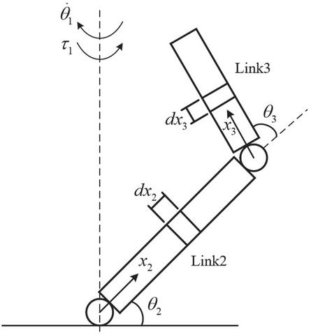
Figure 2 Diagram of normal velocity.

(1) Hydrodynamic resistance moment ${\tau }_{\mathrm{D1}}$ and additional mass moment ${\tau }_{\mathrm{A1}}$ on Joint1 When the Joint1 rotates, the Link2 and the Link3 are driven, so that the Link2 and the Link3 generate a normal velocity, which is perpendicular to the rotation direction of the Joint1. According to the motion relationship between the Link2 and the Link3, the normal velocity is shown in Equation (23)

$$\begin{array}{c}{v}_{2-1}^n={\dot{\theta }}_1{x}_2{c}_2\hfill \\ v_{3-1}^n={\dot{\theta }}_1(a_2{c}_2+x_3{c}_{23})\hfill \end{array}$$

(23)

In which,$v_{2-1}^n,v_{3-1}^n$ are the normal velocities of the Link2 and the Link3 caused by the motion of the Joint1 on the unit length, $x_2$ is the distance from the unit $d{x}_2$ to the bottom of the Link2, $x_3$ and is the distance from the unit $d{x}_3$ to the bottom of the Link3.

Substituting Equations (23) into Equation (20), the hydrodynamic resistance moment of the Joint1 can be obtained, shown in Equation (2.3)

${\tau }_{\mathrm{D1}}$	$={\displaystyle \frac{1}{2}}\rho C_{\mathrm{d}}D[{\displaystyle {\int }_0^{a_2}}{\dot{\theta }}_1{x}_2{c}_2|{\dot{\theta }}_1{x}_2{c}_2|x_2\mathrm{d}{x}_2$
	$\mathrm{\hspace{1em}}+{\displaystyle {\int }_0^{a_3}}{\dot{\theta }}_1(a_2{c}_2+x_3{c}_{23})|{\dot{\theta }}_1(a_2{c}_2+x_3{c}_{23})|(a_2{c}_2+x_3)\mathrm{d}{x}_3]$	(24)

Similarly, the additional mass moment of the Joint1 is shown in Equation (2.3)

${\tau }_{\mathrm{A1}}$	$={\displaystyle \frac{\pi }{4}}\rho C_{\mathrm{m}}{D}^2[{\displaystyle {\int }_0^{a_2}}{x}_2{\displaystyle \frac{\mathrm{d}{\dot{\theta }}_1{x}_2{c}_2}{\mathrm{d}t}}\mathrm{d}{x}_2$
	$+{\displaystyle {\int }_0^{a_3}}(a_2{c}_2+x_3){\displaystyle \frac{\mathrm{d}{\dot{\theta }}_1(a_2{c}_2+x_3{c}_{23})}{\mathrm{d}t}}\mathrm{d}{x}_3]$	(25)

(2) Hydrodynamic resistance moment ${\tau }_{\mathrm{D2}}$ and additional mass moment ${\tau }_{\mathrm{A2}}$ on Joint2 When the Joint2 rotates, the Link2 and the Link3 are driven, so that the Link2 and the Link3 generate a normal velocity, which is perpendicular to the rotation direction of the Joint2. According to the motion relationship between the Link2 and the Link3, the normal velocity is shown in Equation (26)

$$\begin{array}{c}{v}_{2-2}^n={\dot{\theta }}_2{x}_2\hfill \\ v_{3-2}^n={\dot{\theta }}_2{a}_2{c}_3+x_3({\dot{\theta }}_2+{\dot{\theta }}_3)\hfill \end{array}$$

(26)

In which, $v_{2-2}^n,v_{3-2}^n$ are the normal velocities of the Link2 and the Link3 caused by the motion of the Joint2 on the unit length, $x_3$ is the distance from the unit $d{x}_3$ to the bottom of the Link3.

Substituting Equations (26) into Equation (20), the hydrodynamic resistance moment of the Joint2 can be obtained, shown in Equation (2.3)

${\tau }_{\mathrm{D2}}$	$={\displaystyle \frac{1}{2}}\rho C_{\mathrm{d}}D\{{\displaystyle {\int }_0^{a_2}}{\dot{\theta }}_2{x}_2|{\dot{\theta }}_2{x}_2|x_2\mathrm{d}{x}_2$
	$\mathrm{\hspace{1em}}+{\displaystyle {\int }_0^{a_3}}[{\dot{\theta }}_2{a}_2{c}_3+x_3({\dot{\theta }}_2+{\dot{\theta }}_3)]|[{\dot{\theta }}_2{a}_2{c}_3+x_3({\dot{\theta }}_2+{\dot{\theta }}_3)]|$
	$\mathrm{\hspace{1em}}\times (a_2{c}_3+x_3)\mathrm{d}{x}_3\}$	(27)

Similarly, the additional mass moment of the Joint2 is shown in Equation (2.3)

${\tau }_{\mathrm{A2}}$	$={\displaystyle \frac{\pi }{4}}\rho C_{\mathrm{m}}{D}^2\{{\displaystyle {\int }_0^{a_2}}{x}_2{\displaystyle \frac{\mathrm{d}{\dot{\theta }}_2{x}_2}{\mathrm{d}t}}\mathrm{d}{x}_2$
	$+{\displaystyle {\int }_0^{a_3}}(a_2{c}_3+x_3){\displaystyle \frac{\mathrm{d}[{\dot{\theta }}_2{a}_2{c}_3+x_3({\dot{\theta }}_3+{\dot{\theta }}_2)]}{\mathrm{d}t}}\mathrm{d}{x}_3\}$	(28)

(3) Hydrodynamic resistance moment ${\tau }_{\mathrm{D3}}$ and additional mass moment ${\tau }_{\mathrm{A3}}$ on Joint3 When the Joint3 rotates, the Link3 is driven, so that the Link3 generates a normal velocity, which is perpendicular to the rotation direction of the Joint3. According to the motion relationship, the normal velocity is shown in Equation (30)

$$v_{3-3}^n={\dot{\theta }}_2{a}_2{c}_3+x_3({\dot{\theta }}_2+{\dot{\theta }}_3)$$

(29)

Substituting Equations (29) into Equation (20), the hydrodynamic resistance moment of the Joint3 can be obtained, shown in Equation (30)

${\tau }_{\mathrm{D3}}={\displaystyle \frac{1}{2}}\rho C_{\mathrm{d}}D{\displaystyle {\int }_0^{a_3}}[{\dot{\theta }}_2{a}_2{c}_3+x_3({\dot{\theta }}_2+{\dot{\theta }}_3)]|{\dot{\theta }}_2{a}_2{c}_3+x_3({\dot{\theta }}_2+{\dot{\theta }}_3)|x_{3}d{x}_3$

(30)

Similarly, the additional mass moment of the Joint3 is shown in Equation (31)

$${\tau }_{\mathrm{A3}}=\frac{\pi }{4}\rho C_{\mathrm{m}}{D}^2{\int }_0^{a_3}(a_2{c}_3+x_3)\frac{\mathrm{d}[{\dot{\theta }}_2{a}_2{c}_3+x_3({\dot{\theta }}_3+{\dot{\theta }}_2)]}{\mathrm{d}t}d{x}_3$$

(31)

3 Design of Compliant Controller for Underwater Capture System

In order to maintain the operation accuracy of the manipulator during underwater operations, and at the same time show a degree of voluntary compliance to the unknown interference or the impact force of the unmanned underwater vehicle, this study proposes a position-based impedance controller to study the control strategy of the manipulator. During the movement of the manipulator, the error between the actual contact force $F_e$ and the expected contact force $F_d$ of the manipulator will be obtained through the impedance controller, thereby making the manipulator controlled by the position controller. In general, the impedance relationship can be expressed as shown in Equation (32)

$$M_d({\ddot{X}}_e-{\ddot{X}}_d)+B_d({\dot{X}}_e-{\dot{X}}_d)+K_d(X_e-X_d)=F_e-F_d$$

(32)

In which, $M_d$ is the designed inertia matrix, $B_d$ is the designed damping matrix, $K_d$ is the designed stiffness matrix, $X_e,{\dot{X}}_e,{\ddot{X}}_e$ is the actual position, actual velocity, and actual acceleration of the end of the manipulator, and $X_d,{\dot{X}}_d,{\ddot{X}}_d$ is the designed position, designed speed, and designed acceleration of the end of the manipulator.

When the manipulator is impacted by a water flow with a high velocity, a strong impact will be generated due to the inertia of its own motion, which in general does much harm to the mechanical structure of the manipulator. Thus, reasonable adjustment of the target impedance parameters can help reduce the impact of the ocean current on the manipulator, thereby protecting the body structure of the manipulator from damage. According to Equation (32), the target impedance parameters $M_d$, $B_d$, and $K_d$, play a very important role in impedance controller. Generally, since the control system can achieve different control effects by adjusting the value of the impedance parameters, choosing the appropriate impedance parameters is necessary for safe operation.

The larger designed inertia $M_d$ can make the manipulator obtain a relatively great inertia. Considering that the velocity of the manipulator is low when moving underwater, the impact on the actual joints is not remarkable, thus the adjustment effect is not obvious. Larger designed damping $B_d$ can reduce the degree of oscillation of the manipulator. Considering the underwater working environment of the manipulator, the viscous resistance generated by seawater can reduce the degree of oscillation of the manipulator to a certain extent, leading to the fact that the adjustment effect of the designed damping is not obvious enough. The larger the stiffness parameter $K_d$ become, the greater the contact force between the manipulator and the underwater environment is generated. Generally speaking, the adjustment of the stiffness parameter should make the manipulator system in the state of critical damping or over-damping as possible to ensure the instant contact moment in contact with the environment is reduced to a low level.

When the manipulator operates in an underwater environment, it will also be impacted by ocean currents. Moreover, the fluid-structure coupling analysis of the manipulator system needs to be carried out. The hydrodynamic resistance of the manipulator needs to be divided into two parts, one of which is the force generated by its own motion in the still water environment, the other of which is fluid resistance produced by the ocean current impact. When the manipulator operates underwater, it needs to reach a certain level of position tracking accuracy, in order to improve its operation accuracy and ensure its operation stability in the underwater environment.

Compared with the conventional industrial manipulators, the working environment of the underwater manipulator is much more complex, and the measurement of the contact force with the environment can only be calculated by the actual joint torque. Since the effect of hydrodynamic force can be directly reflected on the joint torque sensor, this research will use the value collected by the joint torque sensor and the dynamic model of the manipulator to calculate the hydrodynamic force of the manipulator in statics water, so as to deduce the hydrodynamic force ${\tau }_w$ of each joint in the dynamic water environment to establish the impedance controller of the manipulator in the joint space.

The block diagram of the manipulator’s controller is shown in Figure 3.

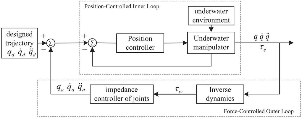
Figure 3 Block diagram of the manipulator’s controller.

4 Simulation Experiment of the Compliant Controller of Underwater Capture System

4.1 Design of the Simulation Experiment

Figure 4 shows the mechanical structure model established by SolidWorks for the underwater capture system consisting of an underwater manipulator and a capture device involved in this study, which has a total of seven degrees of freedom, including three degrees of freedom on the manipulator to adjust the position of capture device, two degrees of freedom on the manipulator to adjusts the tipping and pitching postures of the capture device, as well as two degrees of freedom on the capture device for capture tasks. The structural parameters of underwater manipulator are shown in Table 2.

Figure 4 Schematic diagram of underwater manipulator structure.

Table 2 Parameters table of underwater manipulator’s structure

	Length	Equivalent	Quality	Equivalent	Moment of Inertia
Link $i$	(m)	Diameter (m)	(kg)	Buoyancy (N)	(kg$\cdot$m${}^2$)
Link2	5.0	0.30	530	1420.4	(53.7, 1468.1, 1692.7)
Link3	3.0	0.28	290	750.5	(3.0, 221.1, 222.5)

In the real ocean, the actual underwater environment mostly consists of turbulent, making it difficult to model dynamic of the in manipulator due to the severe uncertainty caused by the separation phenomenon between the motion of the manipulator and the flow around it. In order to simulate the turbulent environment and better simulate the fluctuate time-varying environment of the real ocean, the motion of the manipulator under infinite flow field conditions is simulated with the irregular waves generated in Gaussian white noises model. Based on the relative velocity and relative acceleration of the manipulator with respect to the current during the motion, the hydrodynamic resistance of the manipulator is calculated as a whole and applied to each joint using the Morrison formula derived in Equations (20) and (22) to obtain the equivalent hydrodynamic resistance moment on the joints. The dynamics model of the manipulator is established in Adams, and the equivalent hydrodynamic resistance moment is used to replace the effect of hydrodynamic resistance on the joints of the manipulator and applied to the corresponding joints of the manipulator to simulate a relatively realistic dynamic environment.

In order to study the influence of different impedance parameters on the control system, fixing inertia coefficient $M_d$ damping coefficient $B_d$ and selecting different stiffness coefficient $K_d$ for simulation, the force tracking curves are obtained as shown in Figures 5, 6, and 7.

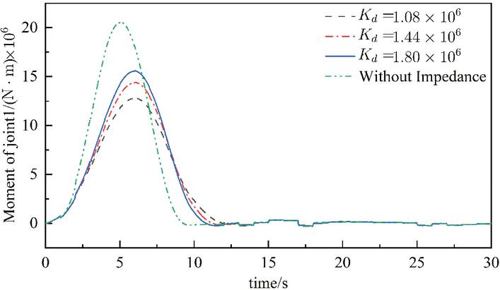
Figure 5 Moment of joint1 with different impedance parameters.

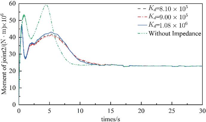
Figure 6 Moment of joint2 with different impedance parameters.

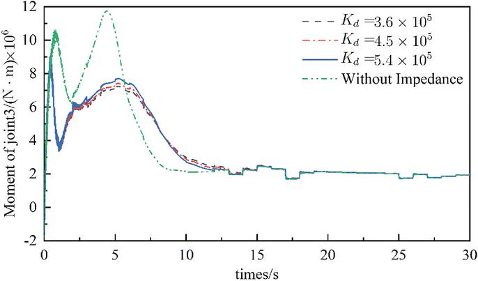
Figure 7 Moment of joint3 with different impedance parameters.

4.2 Analysis of The Simulation Experiment Results

From the comparative analysis of Figures 8, 9 and 10, it can be concluded that in the case of no impedance, the instantaneous contact moment of the underwater manipulator in contact with the environment is relatively large. In the case of the impedance controller, with the increase of the designed stiffness of the joint, the joint moment generated by the manipulator and the water environment will continue to increase. Selecting the appropriate designed stiffness is beneficial to protect the mechanical structure of the underwater manipulator and meet the operational accuracy requirements of the underwater capture system.

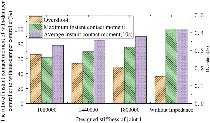
Figure 8 Controller performance index of joint1.

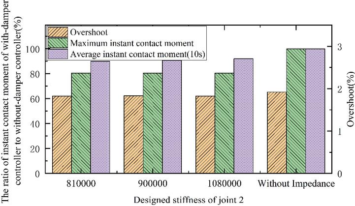
Figure 9 Controller performance index of joint2.

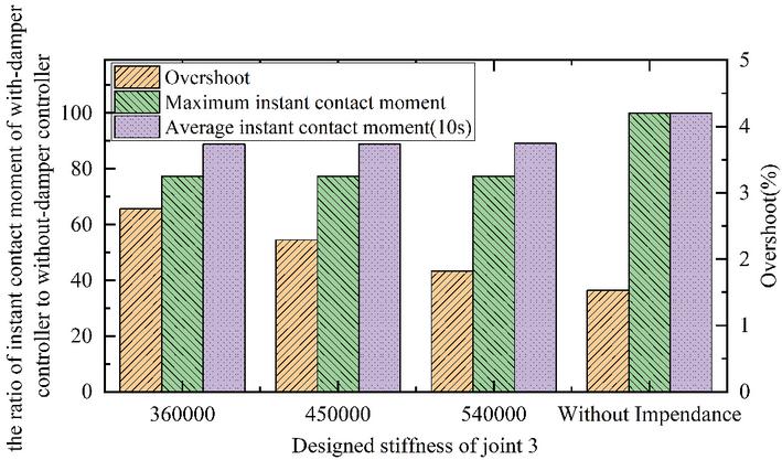
Figure 10 Controller performance index of joint3.

According to the results in Figure 8, the study found that with the increase of the designed stiffness of joint 1, the system overshoot will gradually decrease, but the instant contact force of the manipulator will also gradually increase. Compared with the manipulator with impedance, the maximum instant contact moment and the average contact moment within 10 s of the manipulator without impedance are larger, which proves that the impedance controller is superior in the water environment. Moreover, although the overshoot of the impedance controller is larger than that of the no-impedance case, compared with the reduction of the contact torque, the research believes that the increased overshoot is acceptable compared to the capture accuracy of the system. With the increase of the designed stiffness, the change of overshoot and contact moment produced by the joint 2 are not obvious. It can be considered that for this system, the stiffness coefficient has a poor adjustment effect on the joint 2. However, it is obvious that the overshoot and contact torque of joint 2 will be significantly reduced compared with the case of no impedance. While the designed stiffness is increased, the contact moment generated by the joint 3 does not change significantly, but the overshoot is significantly reduced. It can be considered that appropriately increasing the stiffness of the joint 3 helps to ensure the capture accuracy of the underwater manipulator.

5 Conclusion

Based on the specific structure of the five-degree-of-freedom underwater manipulator, this research analyzes its kinematic model and simplified dynamic model, as well as the hydrodynamic model. According to the characteristics of the underwater environment, a compliance control method based on joint position is designed. The capture system is modeled in Adams dynamics platform to testify the designed compliant controller. The simulation experiment verifies that the compliant controller can reduce the impact of the underwater environment.

For future research, it is believed that the designed stiffness of joint 1 should be appropriately reduced in order to solve the problem of excessive contact force, and the designed stiffness of joint 3 should be appropriately increased to ensure the accuracy of system operation, while the designed stiffness has little adjustment effect on joint 2.

Acknowledgments

This work is supported by the National Natural Science Foundation of China (U2013602, 52075115, 51521003, 61911530250), National Key R&D Program of China (2020YFB13134), Self-Planned Task (SKLRS202001B, SKLRS202110B) of State Key Laboratory of Robotics and System (HIT), Shenzhen Science and Technology Research and Development Foundation (JCYJ20190813171009236), and Basic Scientific Research of Technology (JCKY2020603C009).

References

[1] Chu Z, Xiang X, D Zhu, et al. Adaptive Fuzzy Sliding Mode Diving Control for Autonomous Underwater Vehicle with Input Constraint. International Journal of Fuzzy Systems, 2017. 20: 1460–1469.

[2] GianlucaAntonelli. Fault Detection/Tolerance Strategies for AUVs and ROVs. 2006, 2: 79–91.

[3] Mishra S, Londhe P S, Mohan S, et al. Robust task-space motion control of a mobile manipulator using a nonlinear control with an uncertainty estimator. Computers & Electrical Engineering,, 2018, 67: 729–740.

[4] Liu T, Hu Y, Xu H, et al. Investigation of the vectored thruster AUVs based on 3SPS-S parallel manipulator. Applied Ocean Research, 2019, 85: 151–161.

[5] Lijun Han et al. Adaptive Wave Neural Network Nonsingular Terminal Sliding Mode Control for an Underwater Manipulator with Force Estimation. Transactions of the Canadian Society for Mechanical Engineering, 2020, 45(2): 183–198.

[6] Sangrok Jin et al. Design, modeling and optimization of an underwater manipulator with four-bar mechanism and compliant linkage. Journal of Mechanical Science and Technology, 2016, 30(9): 4337–4343.

[7] M. Santhakumar. A nonregressor nonlinear disturbance observer-based adaptive control scheme for an underwater manipulator. Advanced Robotics, 2013, 27(16): 1273–1283.

[8] Hogan N. Impedance control: An approach to manipulation. Journal of dynamic systems, measurement, and control, 1985, 107(1): 8–16.

[9] Xianjun Sheng, Xi Zhang, Fuzzy adaptive hybrid impedance control for mirror milling system, Mechatronics, 2018, 53: 20–27,

[10] Kang Xu, Shoukun Wang, Binkai Yue, Junzheng Wang, Hui Peng, Dongchen Liu, Zhihua Chen, Mingxin Shi, Adaptive impedance control with variable target stiffness for wheel-legged robot on complex unknown terrain, Mechatronics, 2020, 69, 102388.

[11] Le Liang, Yanyan Chen, Liangchuang Liao, Hongwei Sun, Yanjie Liu, A novel impedance control method of rubber unstacking robot dealing with unpredictable and time-variable adhesion force, Robotics and Computer-Integrated Manufacturing, 2021, 67, 102038.

[12] Ignacio Carlucho, Dylan W. Stephens, Corina Barbalata, An adaptive data-driven controller for underwater manipulators with variable payload, Applied Ocean Research, 2021, 113, 102726.

Biographies

Yuanjie Liu received his bachelor’s degree in Mechanical Design Manufacturing and Automation from Yanshan University, Qinhuangdao, China. He is now pursing his master’s degree in Machinery Engineering at the School of Mechatronic Engineering, Harbin Institute of Technology, Harbin, China. His main research fields are: underwater robots and robots’ dynamic.

Fusheng Zha, associate professor at the School of Mechatronic Engineering, Harbin Institute of Technology. He received his doctorate degree in engineering from Harbin Institute of Technology in 2012. His main research fields are: footed robots, underwater robots, artificial intelligence and self-growing networks, bionic information processing methods, neural information encoding and decoding methods.

Qiming Wang, received his bachelor’s degree in Mechatronic Engineering from Harbin Institute of Technology, and the Master of science degree in Mechanical Engineering from Washington University in St. Louis, the USA. He is now pursing his doctorate degree in mechanical engineering at the School of Mechatronic Engineering, Harbin Institute of Technology. His main research fields are: underwater robots, six-legged robot, robots’ dynamic, and artificial intelligent control methods.

Chao Zheng, is working as an engineer at the Wuhan Second Ship Design and Research Institute, Wuhan, China. His main research area includes underwater robotics and robots’ dynamic.

Jinrui Zhou, is a senior student in Mechatronic Engineering at the School of Mechatronic Engineering, Harbin Institute of Technology. He is going to pursuing his Master’s degree in Mechanical Engineering after graduation. His main contribution to this research is proposing a mechanical design of the manipulator.

Lianzhao Zhang, received his bachelor’s degree in Mechanical and Electronic Engineering from Northwest A&F University, Yangling, China. He is a graduate student pursing master’s degree in Mechanical Engineering at the School of Mechatronic Engineering, Harbin Institute of Technology and is going to pursing his doctorate degree in mechanical engineering. His research interests include the autonomous control, dynamics analysis and simulation of legged robots.

International Journal of Fluid Power, Vol. 24_3, 441–466.
doi: 10.13052/ijfp1439-9776.2432
© 2023 River Publishers

Abstract

1 Introduction

Nomenclature

2 Establishment of the Kinematics and Dynamics Model of the Capture System

2.1 Kinematics Model of the Capture System

2.2 Dynamic Analysis of the Manipulator of the Capture System

2.3 Analysis of the Hydrodynamic Term of the Manipulator of the Capture System

3 Design of Compliant Controller for Underwater Capture System

4 Simulation Experiment of the Compliant Controller of Underwater Capture System

4.1 Design of the Simulation Experiment

4.2 Analysis of The Simulation Experiment Results

5 Conclusion

Acknowledgments

References

Biographies