Study of Hydrodnamic Pumping Effects of Fixed Axis Rotation in Eccentric Annular Flow Field

Tong Guo^{1, 2, 3}, Tao Luo¹, Tianliang Lin^{1, 3,}*, Qihuai Chen^{1, 3}, Haoling Ren^{1, 3} and Yuanhua Yu⁴

¹Huaqiao University, Xiamen, Fujian 361021 China
²State Key Laboratory of Fluid Power and Mechatronic Systems, Zhejiang University, Hangzhou 310027 China
³Fujian Key Laboratory of Green Intelligent Drive and Transmission for Mobile Machinery, Xiamen 361021, China
⁴Beijing BinanHX Control Technology Co., Ltd., Beijing, 100176, China
E-mail: ltlkxl@163.com
*Corresponding Author

Received 22 May 2022; Accepted 27 August 2022; Publication 12 June 2023

Abstract

Hydrodynamic effect is one of the key phenomena in journal bearing lubrication. Many researches have been carried out on the supporting force of journal bearing, the motion of suspension shaft and the lubrication effect. This paper studies the hydrodynamic effect from another point of view, that is, the pumping effect caused by the rotation of the eccentric shaft with fixed axis. The clearance between the rotor and the stator is divided into two sections by the inlet port and the outlet port. Their mathematical models are established and studied in polar coordinates. The pressure distribution and pumping flowrate in the flow field are studied theoretically. Under the conditions analyzed in this paper, an output flow larger than 90 ml/s could be generated, overcoming a load pressure of 0.5 MPa. In addition, the pressure distribution and pumping flowrate of the mechanism are affected by the pumping outlet orientation. According to the analysis results of the output angle range from $\pi$/8 to 3$\pi$/4, when the pump outlet angle is set near 3$\pi$/8 to $\pi$/2, the pumping flowrate reaches the maximum value of 91.83 ml/s, and nearly half 48% of the inflow liquid can be pumped out to the outlet.

Keywords: Pumping effect, hydrodynamic effect, eccentric annular clearance, mathematical model.

1 Introduction

Hydrodynamic effect has been studied since the famous bearing friction experiments designed by Beauchamp Tower in 1880s. Based on his findings, Osborn Reynolds established the fundamental theory of hydrodynamic lubrication which describes the basic mechanism within the journal bearing, and then solving the Reynolds’ equations became to be one of the key steps of the designing and optimizing of bearings [1–3]. After years’ studies on this specific phenomenon in the clearance flow field, many results as well as scientific branches have evolved, including elasto-hydrodynamic lubrication (EHL), thermo-hydrodynamic lubrication and the turbulent flow theories [4]. HL refers to the lubrication when the elastic deformation of the contact surface has an nonnegligible influence on the lubricating film thickness [5]. It has important influence on the designing and calculation of rolling bearing, gears and synovial joints. Hamrock presented the most widely applied formula to calculated the film thickness in 1976 [6]. After Nijenbanning put forward a more accurate equation in 1994, the research focus of the EHL turned to the incomplete oil film [7]. Thermo-hydrodynamic lubrication (THL) is also a significant branch of lubrication theory which take the heat generation and temperature rise on the fluid into consideration. Researchers focus on the accurate establishment of mathematical model and the calculation of viscosity, density and other physical parameters caused by temperature effect, as well as the temperature distribution in the liquid film and their influence on hydrodynamic lubrication. Dowson conducted a major experiment to reveal the thermal characteristics of journal bearings including the heat flow patterns and the temperature distributions [8]. Shan proposed a theoretical framework for representing hydrodynamic systems based on Boltzmann equation to supplement the traditional Navier–Stokes equation [9]. Based on the previous findings, Singh accomplished a simultaneous analysis of the fluid film of a journal bearing under steady-state [10]. It is generally believed that when the Reynolds number reaches about 1000, the flow state of the thin liquid film will change from laminar flow to turbulent flow. Therefore, in some large-scale, high-speed bearing analysis, the flow state of the fluid should be considered as turbulence. Many methods have been proposed to solve turbulence problems, including time-average equation [11], mixing length theory [12] and K-means method-$\epsilon$ Model, etc [1].

The main focuses of the researches are based on the application occasion of journal bearing. The rotation flow field are formed and governed by a levitated bearing rod centered in the sleeve, and the position and eccentricity of the axis of the rod and the liquid thickness are varying with the rotating of the shaft. The generated hydrodynamic pressure is used to support the rod to separated it from the sleeve to prevent wearing. The authors notice that the generated pressure is countable to overcome certain outlet resistances to form an output flow. Therefore, it would be interesting to study the hydrodynamic effect from the perspective of pumping capacity and this pumping effect may be potential to be used to drive high-vicious fluid or to develop micropumps.

Nomenclature

$\rho$	Density of the fluid
$u$	Flow velocity of the fluid
$r$	Radial coordinate
$u_r$	Radial velocity
$u_{\theta }$	Circumferential velocity
$\theta$	Rotation angle
$P$	Fluid pressure
$\nu$	Kinematic viscosity
$a_r$	Radial acceleration
$a_{\theta }$	Circumferential acceleration
${\rho }_0$	Relative unit: a typical fluid density
$r_0$	Relative unit: a typical radius
$h_0$	Relative unit: a typical fluid film thickness
$V_0$	Relative unit: a typical radial velocity
${\theta }_0$	Relative unit: a typical rotation angle
$U_0$	Relative unit: a typical circumferential velocity
${\nu }_0$	Relative unit: a typical kinematic viscosity
$P_0$	Relative unit: a typical pressure
$\overline{\rho }$	Dimensionless variables: fluid density
$\overline{r}$	Dimensionless variables: radius
$\overline{h}$	Dimensionless variables: fluid film thickness
$\overline{u_r}$	Dimensionless variables: radial velocity
$\overline{\theta }$	Dimensionless variables: rotation angle
$\overline{u_{\theta }}$	Dimensionless variables: circumferential acceleration
$\overline{\nu }$	Dimensionless variables: kinematic viscosity
$\overline{P}$	Dimensionless variables: pressure
$q_{\mathit{pump}}$	Pumping flowrate
$q_1$	Inlet flowrate
$q_2$	Leakage flowrate
$h_{\theta }$	Fluid film thickness at angle $\theta$
$h_m$	Film thickness where the pressure gradient is zero
$c$	Radial clearance (the difference between the radius of the stator
	and the rotor
$e$	Eccentricity between the rotor and the stator
$\epsilon$	Radial gap offset ratio (the ratio of eccentricity to $c$)
$P_{\mathit{inlet}}$	Inlet pressure
$P_{\mathit{pump}}$	Pumping pressure
$n$	Rotation speed

2 Basic Descriptions and Mathematic Models

2.1 Basic Geometry, Scheme and Assumptions

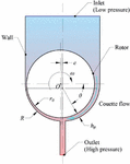
This paper aims to discuss the hydrodynamic pumping effect of the flow in the eccentric annular clearance. The basic structure of the flow field is simple, as shown in Figure 1. The circular rotor with fixed axis is eccentrically installed in the stator. The two ports of the stator chamber are respectively connected with a low-pressure inlet and a high-pressure outlet. The stator cavity is filled with fluid. Because of the viscosity of the fluid, when the rotor rotates around its fixed axis, the fluid near the outer wall of the rotor will be driven to form a couette flow. In the eccentric annular gap (lower part) composed of rotor and stator, as shown in Figure 1, the couette flow enters the larger port and flows out of the smaller port, which meets the formation conditions of hydrodynamic pressure. Therefore, the fluid pressure is increased in the process. When the hydrodynamic pressure is higher than the pressure difference between the inlet and outlet, it will be possible to pump the fluid out of the outlet. This pumping effect may be used to transport high viscous fluid or to generate a micro flow. In addition, because of its very simple structure, it can be used to design micro pumps with long service life.

Figure 1 Basic geometry of the hydrodynamic pumping flow field.

The difference between the hydrodynamic pumping effect considered in this paper and the well-studied hydrodynamic support and lubrication in journal bearings includes:

1. Transmission structures: the rotor of journal bearing is suspended and supported in the stator. When the rotor rotates, it will move circumferentially and radially under the constraint of the stator. As for the case discussed in this paper, the rotor axis is fixed.

2. Dynamic flow field: the hydrodynamic pressure in journal bearing is utilized to overcome the radial load of the rotor and separate rotor and stator, to avoid dry friction. For the rotor with fixed axis, the eccentric annulus is filled with fluid, and the hydrodynamic pressure is used to overcome the outlet resistance to form a continuous flow.

This paper presents a preliminary study on hydrodynamic pumping effect. The basic mathematical model is established and the pumping characteristics of pressure and flowrate are analyzed theoretically.

In the mathematical derivation in this paper, the following assumptions are adopted:

1. The flow is 2D, steady and laminar.

2. The gravity can be ignored compared with the viscous force.

3. Compressibility of the fluid is negligible.

4. The fluid is Newtonian and the coefficient of viscosity is constant.

5. Fluid pressure does not change across the film thickness.

2.2 2D-Mathematic Models and Derivation of Reynolds Equation in Polar Coordinates

The hydrodynamic effect functions in the contraction area in the lower part of Figure 1. The continuity equation and momentum conservation equation of the flow field could be written based on polar coordinates as follows:

$$\nabla \cdot \rho \mathrm{u}=\frac{1}{\mathrm{r}}\left[\frac{\partial (\rho {\mathrm{u}}_{\mathrm{r}}\mathrm{r})}{\partial \mathrm{r}}+\frac{\partial \rho {\mathrm{u}}_{\theta }}{\partial \theta }\right]=0$$

(1)

$$\{\begin{array}{c}-\frac{1}{\rho }\frac{\partial \mathrm{P}}{\partial \mathrm{r}}+\nu \left[\frac{1}{\mathrm{r}}\frac{\partial }{\partial \mathrm{r}}\left(\mathrm{r}\frac{\partial {\mathrm{u}}_{\mathrm{r}}}{\partial \mathrm{r}}\right)+\frac{1}{{\mathrm{r}}^2}\frac{{\partial }^2{\mathrm{u}}_{\mathrm{r}}}{\partial {\theta }^2}-\frac{{\mathrm{u}}_{\mathrm{r}}}{{\mathrm{r}}^2}-\frac{2}{{\mathrm{r}}^2}\frac{\partial {\mathrm{u}}_{\theta }}{\partial \theta }\right]={\mathrm{a}}_{\mathrm{r}}\hfill \\ -\frac{1}{\mathrm{r}\rho }\frac{\partial \mathrm{P}}{\partial \theta }+\nu \left[\frac{1}{\mathrm{r}}\frac{\partial }{\partial \mathrm{r}}\left(\mathrm{r}\frac{\partial {\mathrm{u}}_{\theta }}{\partial \mathrm{r}}\right)+\frac{1}{{\mathrm{r}}^2}\frac{{\partial }^2{\mathrm{u}}_{\theta }}{\partial {\theta }^2}-\frac{{\mathrm{u}}_{\theta }}{{\mathrm{r}}^2}+\frac{2}{{\mathrm{r}}^2}\frac{\partial {\mathrm{u}}_{\mathrm{r}}}{\partial \theta }\right]={\mathrm{a}}_{\theta }\hfill \end{array}$$

(2)

In Equation (2), $a_r$ and $a_{\theta }$ could be expanded as below:

$$\{\begin{array}{c}{\mathrm{a}}_{\mathrm{r}}={\mathrm{u}}_{\mathrm{r}}\frac{\partial {\mathrm{u}}_{\mathrm{r}}}{\partial \mathrm{r}}+\frac{{\mathrm{u}}_{\theta }}{\mathrm{r}}\cdot \frac{\partial {\mathrm{u}}_{\mathrm{r}}}{\partial \theta }-\frac{{\mathrm{u}}_{\theta }^2}{\mathrm{r}}\hfill \\ {\mathrm{a}}_{\theta }={\mathrm{u}}_{\mathrm{r}}\frac{\partial {\mathrm{u}}_{\theta }}{\partial \mathrm{r}}+\frac{{\mathrm{u}}_{\theta }}{\mathrm{r}}\cdot \frac{\partial {\mathrm{u}}_{\theta }}{\partial \theta }+\frac{{\mathrm{u}}_{\mathrm{r}}{\mathrm{u}}_{\theta }}{\mathrm{r}}\hfill \end{array}$$

(3)

Table 1 Variable substitution table of continuity equation

Variable	Relative Unit	Expression
$\rho$	${\rho }_0$	$\rho =\overline{\rho }\cdot {\rho }_0$
$r$	$r_0$	$r=\overline{r}\cdot r_0$
$\partial r$	$h_0$	$\partial r=\partial h=\partial \overline{h}\cdot h_0$
$u_r$	$V_0$	$u_r=\overline{u_r}\cdot V_0$
$\theta$	${\theta }_0$	$\theta =\overline{\theta }\cdot {\theta }_0$

By introducing the substitution shown in Table 1, Equation (1) can be rewritten in relative units and dimensionless quantities with uniform order of magnitude, as shown by Equation (4).

$$\frac{1}{\overline{\mathrm{r}}\cdot {\mathrm{r}}_0}\cdot \frac{\partial (\overline{\rho }\cdot {\rho }_0\cdot \overline{{\mathrm{u}}_{\mathrm{r}}}\cdot {\mathrm{V}}_0\cdot \overline{\mathrm{r}}\cdot {\mathrm{r}}_0)}{\partial (\overline{\mathrm{h}}\cdot {\mathrm{h}}_0)}+\frac{1}{\overline{\mathrm{r}}\cdot {\mathrm{r}}_0}\cdot \frac{\partial (\overline{\rho }\cdot {\rho }_0\cdot \overline{{\mathrm{u}}_{\theta }}\cdot {\mathrm{U}}_0)}{\partial (\overline{\theta }\cdot {\theta }_0)}=0$$

(4)

In which, the relative units ${\rho }_0$, $r_0$, $V_0$, ${\theta }_0$ and $U_0$ are some typical values of the variables. Apparently, $h_0$ is far smaller than $r_0$, namely $\frac{h_0}{r_0}=\psi \ll 1$. By multiplying $\frac{r_0}{U_0}$ on both sides of Equation (4), it can be transformed into:

$$\frac{{\mathrm{V}}_0}{{\mathrm{U}}_0}\cdot \frac{{\mathrm{r}}_0}{{\mathrm{h}}_0}\cdot \frac{1}{\overline{\mathrm{r}}}\cdot \frac{\partial (\overline{\rho }\cdot \overline{{\mathrm{u}}_{\mathrm{r}}}\cdot \overline{\mathrm{r}})}{\partial \overline{\mathrm{h}}}+\frac{1}{\overline{\mathrm{r}}}\cdot \frac{\partial (\overline{\rho }\cdot \overline{{\mathrm{u}}_{\theta }})}{\partial (\overline{\theta }\cdot {\theta }_0)}=0$$

(5)

Since the order of magnitude of the second term in Equation (4) is 1, according to the theory of magnitude homogeneity, the order of magnitude of the first term should also be 1. Therefore, $O(\frac{V_0}{U_0})=\psi \ll 1$, which infers that the momentum in the radial direction is much less than that in the circumferential direction and the radial momentum equation can be ignored.

Table 2 Variable substitution table of momentum equation

Variable	Relative Unit	Expression
$\nu$	${\nu }_0$	$\nu =\overline{\nu }\cdot {\nu }_0$
$P$	$P_0$	$P=\overline{P}\cdot P_0$

Similarly, by introducing the substitution in Table 2, the circumferential momentum in Equation (2) can be rewritten as Equation (6).

	$-{\displaystyle \frac{h_0^2}{{\nu }_0\cdot U_0}}\cdot {\displaystyle \frac{P_0}{r_0\cdot {\rho }_0}}\cdot {\displaystyle \frac{1}{\overline{r}\cdot \overline{\rho }}}\cdot {\displaystyle \frac{\partial \overline{P}}{\partial (\overline{\theta }\cdot {\theta }_0)}}$	(6)
	$+\overline{\nu }\cdot [{\displaystyle \frac{1}{\overline{r}}}\cdot {\displaystyle \frac{\partial }{\partial \overline{h}}}(\overline{r}\cdot {\displaystyle \frac{\partial \overline{u_{\theta }}}{\partial \overline{h}}})+{\displaystyle \frac{h_0^2}{r_0^2}}\cdot {\displaystyle \frac{1}{{\overline{r}}^2}}\cdot {\displaystyle \frac{{\partial }^2\overline{u_{\theta }}}{\partial {(\overline{\theta }\cdot {\theta }_0)}^2}}-{\displaystyle \frac{h_0^2}{r_0^2}}\cdot {\displaystyle \frac{\overline{u_{\theta }}}{{\overline{r}}^2}}$
	$+{\displaystyle \frac{2h_0^2}{r_0^2}}\cdot {\displaystyle \frac{1}{{\overline{r}}^2}}\cdot {\displaystyle \frac{\partial \overline{u_r}}{\partial \left(\overline{\theta }\cdot {\theta }_0\right)}}]$
	$={\displaystyle \frac{h_0\cdot V_0}{{\nu }_0}}\cdot \overline{u_r}\cdot {\displaystyle \frac{\partial \overline{u_{\theta }}}{\partial \overline{h}}}+{\displaystyle \frac{h_0^2}{{\nu }_0}}\cdot {\displaystyle \frac{U_0}{r_0}}\cdot {\displaystyle \frac{\overline{u_{\theta }}}{\overline{r}}}\cdot {\displaystyle \frac{\partial \overline{u_{\theta }}}{\partial \left(\overline{\theta }\cdot {\theta }_0\right)}}+{\displaystyle \frac{h_0^2}{{\nu }_0}}\cdot {\displaystyle \frac{V_0}{r_0}}\cdot {\displaystyle \frac{\overline{u_r}\cdot \overline{u_{\theta }}}{\overline{r}}}$

In which, $O(\frac{h_0^2}{r_0^2})={\psi }^2$, $O(\frac{h_0\cdot V_0}{r_0\cdot U_0})={\psi }^2$, $O(\frac{2h_0^2{V}_0}{r_0^2{U}_0})={\psi }^3$, after ignoring these small quantities, Equation (6) could be simplified as below:

$\begin{array}{cc}& -{\displaystyle \frac{{\mathrm{h}}_0^2}{{\nu }_0\cdot {\mathrm{U}}_0}}\cdot {\displaystyle \frac{{\mathrm{P}}_0}{{\mathrm{r}}_0\cdot {\rho }_0}}\cdot {\displaystyle \frac{1}{\overline{\mathrm{r}}\cdot \overline{\rho }}}\cdot {\displaystyle \frac{\partial \overline{\mathrm{P}}}{\partial \left(\overline{\theta }\cdot {\theta }_0\right)}}+\overline{\nu }\cdot \left[{\displaystyle \frac{1}{\overline{\mathrm{r}}}}\cdot {\displaystyle \frac{\partial }{\partial \overline{\mathrm{h}}}}\left(\overline{\mathrm{r}}\cdot {\displaystyle \frac{\partial \overline{{\mathrm{u}}_{\theta }}}{\partial \overline{\mathrm{h}}}}\right)\right]\hfill \\ & ={\displaystyle \frac{{\mathrm{h}}_0\cdot {\mathrm{U}}_0}{{\nu }_0}}\cdot {\displaystyle \frac{{\mathrm{h}}_0}{{\mathrm{r}}_0}}\cdot \left[{\displaystyle \frac{{\mathrm{r}}_0}{{\mathrm{h}}_0}}\cdot {\displaystyle \frac{{\mathrm{V}}_0}{{\mathrm{U}}_0}}\cdot \overline{{\mathrm{u}}_{\mathrm{r}}}\cdot {\displaystyle \frac{\partial \overline{{\mathrm{u}}_{\theta }}}{\partial \overline{\mathrm{h}}}}+{\displaystyle \frac{\overline{{\mathrm{u}}_{\theta }}}{\overline{\mathrm{r}}}}\cdot {\displaystyle \frac{\partial \overline{{\mathrm{u}}_{\theta }}}{\partial (\overline{\theta }\cdot {\theta }_0)}}+{\displaystyle \frac{{\mathrm{V}}_0}{{\mathrm{U}}_0}}\cdot {\displaystyle \frac{\overline{{\mathrm{u}}_{\mathrm{r}}}\cdot \overline{{\mathrm{u}}_{\theta }}}{\overline{\mathrm{r}}}}\right]\hfill \end{array}$

When the Reynolds number satisfies $Re=\frac{h_0\cdot U_0}{{\nu }_0}\ll \frac{1}{\psi }$, then $\frac{h_0\cdot U_0}{{\nu }_0}\cdot \frac{h_0}{r_0}\ll 1$, which infers that the inertia term can be ignored. So, Equation (7) could be change into Equation (8).

$$\frac{{\mathrm{h}}_0^2}{{\nu }_0\cdot {\mathrm{U}}_0}\cdot \frac{{\mathrm{P}}_0}{{\mathrm{r}}_0\cdot {\rho }_0}\cdot \frac{1}{\overline{\mathrm{r}}\cdot \overline{\rho }}\cdot \frac{\partial \overline{\mathrm{P}}}{\partial (\overline{\theta }\cdot {\theta }_0)}=\overline{\nu }\cdot \frac{1}{\overline{\mathrm{r}}}\cdot \frac{\partial }{\partial \overline{\mathrm{h}}}\left(\overline{\mathrm{r}}\cdot \frac{\partial \overline{{\mathrm{u}}_{\theta }}}{\partial \overline{\mathrm{h}}}\right)$$

(8)

By restoring Equation (8) into the normal variable mode and ignore the difference between $r$ and $r_0$, the Reynolds equation in polar coordinates is obtained as shown by Equation (9).

$$\frac{\partial \mathrm{P}}{\partial \theta }=\mu \cdot {\mathrm{r}}_0\cdot \frac{{\partial }^2{\mathrm{u}}_{\theta }}{\partial {\mathrm{h}}^2}$$

(9)

3 Solutions of the Pressure Distributions and Flowrates

3.1 Three Flows Around the Conjunction Area

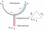
There are three main flow streams in the hydrodynamic region: $q_1$, $q_2$ and $q_{\mathit{pump}}$. $q_1$ consists of two different sorts of flows with opposite flow directions. One is the Couette flow caused by the rotation of the rotor, and the other is caused by the pressure difference between the inlet and outlet. Only when the couette flow is greater than the differential pressure flow, $q_1$ will flow from inlet to outlet. $q_2$ is also composed of couette flow and differential pressure flow, however the flow directions of theirs are consistent. $q_{\mathit{pump}}$ is the flow pumped out through the outlet by hydrodynamic pressure. $q_1$, $q_2$ and $q_{\mathit{pump}}$ satisfy Equation (10).

$${\mathrm{q}}_{\mathrm{pump}}={\mathrm{q}}_1-{\mathrm{q}}_2$$

(10)

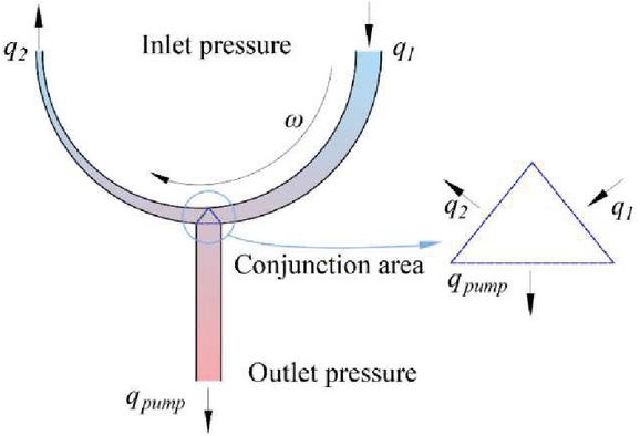
Figure 2 Flows in the hydrodynamic regions.

3.2 Solutions of the Flowrate of Hydrodynamic Pressure Distribution

In the two eccentric annuli on both sides of the conjunction region, $q_1$ and $q_2$ obey the continuity Equation (1) and momentum conservation Equation (9). By integrating Equation (9) twice in the direction of the thickness of the fluid film, the expression of circumferential velocity can be obtained as follows:

$${\mathrm{u}}_{\theta }=\frac{1}{2\mu \cdot {\mathrm{r}}_0}\cdot \frac{\partial \mathrm{P}}{\partial \theta }\cdot \mathrm{h}\cdot (\mathrm{h}-{\mathrm{h}}_{\theta })-\frac{\mathrm{U}}{{\mathrm{h}}_{\theta }}(\mathrm{h}-{\mathrm{h}}_{\theta })$$

(11)

In which, $h_{\theta }$ indicates the thickness of the liquid film at the rotation angle of $h_{\theta }$ and $U$ is the linear velocity on the rotor surface. Furthermore, the circumferential flowrate can be obtained by integrating $u_{\theta }$ in the direction of fluid film thickness, as shown by Equation (12).

${\mathrm{q}}_{\theta }$	$={\displaystyle {\int }_0^{{\mathrm{h}}_{\theta }}}{\mathrm{u}}_{\theta }\mathrm{dh}$	(12)
	$={\displaystyle {\int }_0^{{\mathrm{h}}_{\theta }}}\left({\displaystyle \frac{1}{2\mu \cdot {\mathrm{r}}_0}}\cdot {\displaystyle \frac{\partial \mathrm{P}}{\partial \theta }}\cdot \mathrm{h}\cdot \left(\mathrm{h}-{\mathrm{h}}_{\theta }\right)-{\displaystyle \frac{\mathrm{U}}{{\mathrm{h}}_{\theta }}}\left(\mathrm{h}-{\mathrm{h}}_{\theta }\right)\right)\mathrm{dh}$
	$={\displaystyle \frac{{\mathrm{Uh}}_{\theta }}{2}}-{\displaystyle \frac{{\mathrm{h}}_{\theta }^3}{12\mu \cdot {\mathrm{r}}_0}}\cdot {\displaystyle \frac{\partial \mathrm{P}}{\partial \theta }}$

Discussion: According to the general steps of derivation and simplification of Reynolds equation, it is necessary to integrate the continuity equation in the direction of fluid thickness and substitute the circumferential and radial flow expressions into the integration results. Then, considering that the radial flow is far smaller than the circumferential flow, the radial flowrate could be ignored and the one-dimensional Reynolds equation in the circumferential direction is obtained. Furthermore, by integrating the equation in the circumferential direction, the integral form of one-dimensional Reynolds equation, namely the expression of the circumferential pressure gradient is obtained. However, this article adopts a shortcut. Since the radial flow is negligible, the circumferential flowrate $q_{\theta }$ should be constant. By introducing the film thickness $q_{\theta }$ at the position where the pressure gradient is zero (${\frac{dP}{d\theta }|}_{\theta =m}=0$), the pressure gradient equation can be obtained directly, as shown by Equation (13).

$$\frac{\mathrm{dP}}{\mathrm{d}\theta }=6\mu {\mathrm{r}}_0\mathrm{U}\cdot \frac{{\mathrm{h}}_{\theta }-{\mathrm{h}}_{\mathrm{m}}}{{\mathrm{h}}_{\theta }^3}$$

(13)

By introducing the fluid film thickness expression as shown by Equation (14), the pressure distribution could be calculated as Equation (15) [1].

$$\mathrm{h}(\theta )=\mathrm{c}(1+\epsilon \cdot \cos \theta )$$

(14)

$$\begin{array}{cc}\hfill \mathrm{P}(\theta )& =\frac{6\mu {\mathrm{r}}_0\mathrm{U}}{{\mathrm{c}}^2}[\frac{\theta -\epsilon \cdot \sin \theta }{{(1-{\epsilon }^2)}^{\frac{3}{2}}}-\frac{{\mathrm{h}}_{\mathrm{m}}}{\mathrm{c}{(1-{\epsilon }^2)}^{\frac{5}{2}}}\hfill \\ & \cdot (\theta -2\epsilon \cdot \sin \theta +\frac{{\epsilon }^2\theta }{2}+\frac{{\epsilon }^2}{4}\mathrm{sin2}\theta )]+\mathrm{C}\hfill \end{array}$$

(15)

According to Figure 1, Figure 2 and the basic consumptions, the contraction part in the annular clearance could be regarded as two hydrodynamic regions both satisfying the half-Sommerfeld conditions and their boundary conditions are as follows:

$$\{\begin{array}{cc}\mathrm{P}={\mathrm{P}}_{\mathrm{inlet}},\hfill & \theta =0\mathit{\hspace{1em}}\mathrm{and}\mathit{\hspace{1em}}\theta =\pi \hfill \\ \mathrm{P}={\mathrm{P}}_{\mathrm{pump}},\hfill & \theta =\pi /2\hfill \end{array}$$

(16)

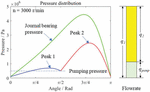
By substituting the above boundary conditions into Equation (15), the constants $h_m$ and $c$ of the pressure distribution corresponding to the two hydrodynamic regions can be obtained respectively. Furthermore, adopting the basic parameters listed in Table 3, the flowrates and the pressure distributions described by Equations (12) and (15) can be obtained and shown in Figure 3. The pressure of journal bearing is also plotted for comparison.

Table 3 The basic parameters of pumping mechanism

Variable	Relative Unit
${\mathrm{r}}_0/\mathrm{mm}$	10
$R/\mathrm{mm}$	10.1
$e/\mathrm{mm}$	0.05
$\epsilon$	0.5
n/r/min	3000
$v/{\mathrm{mm}}^2/s$	410.9
$\rho /\mathrm{kg}/{\mathrm{m}}^3$	892
$P_{\mathit{pump}}/\mathrm{MPa}$	0.5

Figure 3 Sketch of the pressure distribution and the flowrate.

As shown in Figure 3 in the two hydrodynamic pressure zones before and after $\theta =\pi /2$, there are pressure variation that is similar to those in journal bearings. These two pressure peaks have important influences on the pumping effect. The pressure rise before $\pi$/2 is the motive force of pumping fluid, while the pressure rise after $\pi$/2 is the resistance of the fluid leakage. Apparently, increasing peak 1 and peak 2 are both beneficial to enhance the pumping capacity of the mechanism. On the other hand, the values of the two peaks depend on the angle position of the pump outlet, and when the outlet angle is greater than $\pi$/2, the peak 1 will increase and the peak 2 will decrease$;$ on the contrary, when the exit angle is less than $\pi$/2, the peak 1 will decrease and the peak 2 will increase.

4 Preliminary Optimization of Pumping Effect

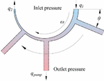
To study the influence of different outlet position on pumping flowrate, a series of studies were carried out. The pumping angle varies from $\pi$/8 to 3$\pi$/4 as shown in Figure 4.

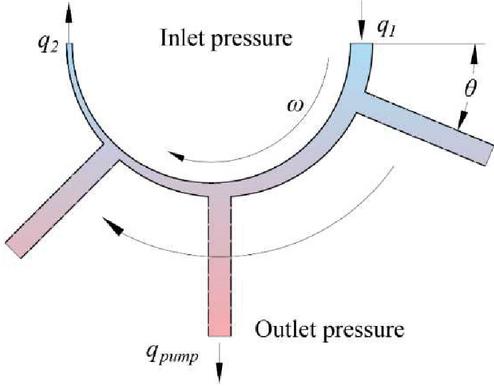
Figure 4 Preliminary optimization of pumping effect.

According to the calculation results shown by Table 4 and Figure 5, under the same outlet load pressure, with the increase of outlet angle, the output flow and its proportion in the total inflow increase firstly and then decrease, and reach peak values near the angle of 3$\pi$/8 to $\pi$/2. The highest pumping efficiency can reach nearly 50%. The analysis results can be explained as follows: the pressure rise in the inlet section has two effects: (1) enhance the liquid pumping out to the outlet; (2) prevent the liquid from flowing into the annulus. Since the pumping flow only accounts for a part of the inflow, the latter of the above effects plays the major role. Correspondingly, the pressure peak of the leakage outflow section also has two effects: (1) prevent the fluid flowing into the leakage section from the conjunction area; (2) accelerate the leakage of fluid. Since the conjunction zone is the source of the liquid of the leakage section, the former of the above effects plays the major role. To sum up, to enhance the hydrodynamic pumping effect, it seems to be appropriate to increase the peak pressure in the leakage section as much as possible, and remain a pressure slightly higher than the pumping pressure in the inflow section.

Table 4 Calculation results of different pumping angle

Angle	Inlet Flow	Leakage Flow	Pumping Flow	Pumping
(rad)	(ml/s)	(ml/s)	(ml/s)	Efficiency
$\pi /8$	139.2	103.9	35.35	25%
$\pi /4$	183.8	101.5	82.29	45%
$3\pi /8$	190.6	98.77	91.83	48%
$\pi /2$	182.7	95.41	87.33	48%
$5\pi /8$	164.8	91.31	73.53	45%
$3\pi /4$	141.1	86.81	54.29	38%

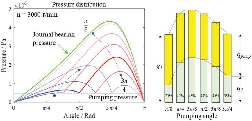
Figure 5 Pressure distributions and flow rates under different pumping angles.

5 Simulation Studies

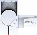
Computational Fluid Dynamics (CFD) analyses with pumping angles from 3$\pi$/8 to $\pi$/2 are conducted based on Ansys Fluent [13], to investigate the flow field characteristics of the model. Basic parameters listed in Table 3 are adopted and the quadrilateral dominated meshes are drawn, as shown in Figure 6. The total number of grids is 49101, the number of layers at the thinnest is 10, and the average quality of grids is 0.99. Grid independence is verified. The simulation model and boundary condition settings are shown in Table 5.

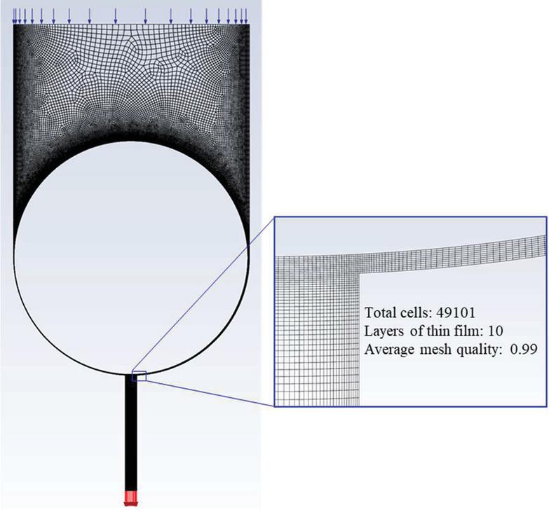
Figure 6 Quadrilateral dominated mesh for CFD simulations.

Table 5 Simulation settings for CFD analysis

Models and Parameters	Settings
Solver	Pressure-Based, steady
Multiphase	No
Viscous Model	k-epsilon, RNG
Solution Methods	Coupled
Pressure inlet (Pa)	0
Pressure outlet (Pa)	5 $\times$ 10${}^5$
Reference pressure (Pa)	101325
Rotation speed (rad/s)	314.16
Operating fluid	14# lubricating oil

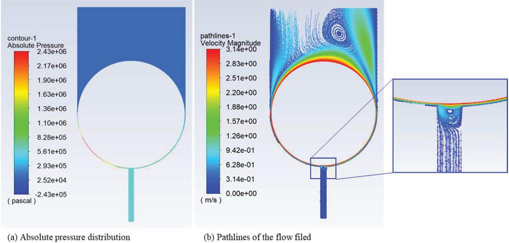
Figure 7 CFD simulation results with pumping angle of $\pi$/2.

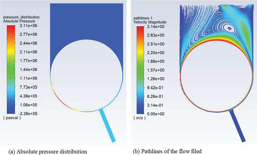
Figure 8 CFD simulation results with pumping angle of 3$\pi$/8.

The pressure contours and streamlines of the flow fields with pumping angles of $\pi$/2 and 3$\pi$/8 are shown by Figures 7 and 8. Figures 7(a) and 8(a) indicate that the highest pressure occurs at the rear section of hydrodynamic pressure region and the model with 3$\pi$/8 pumping angle can form an even higher pressure than that with pumping angle of $\pi$/2, due to the longer pressure boost length in the high-pressure region. The peak pressures can reach 2.43 MPa and 3.11 MPa respectively. Figures 7(b) and 8(b) depict the streamline in the flow field, colored with absolute velocity. It is shown that two types of vortices will appear at the inlet and outlet of the flow field, which should be caused by the combined effect of the drag of the rotor on the fluid and the pressure difference.

The pressure distributions of the hydrodynamic regions of the CFD simulations as well as the theoretical are plotted in Figure 9. Both simulation results of models with the two different pumping angles are in good agreement with the theoretical values. The pumping flowrates can reach 97.4 ml/s and 94.2 ml/s respectively, accounting for 49% and 50% of the total flow q1. The above analysis suggests that the mathematic model established in this paper is available and the pumping capacity is of practical value.

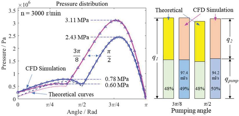
Figure 9 Comparisons of pressure distributions and flow rates.

6 Limitations

This article focuses on the pumping effect of the dynamic pressure in the eccentric clearance region. The mathematic modelling and simulation study are based on 2D assumption. Thus, the influences on the pressure distribution as well as the flowrate caused by the both lateral ends of an actual organization are ignored. In the simulation studies, it is captured that the impossible negative absolute pressure occurs where the angle is slightly greater than $\pi$, which should be considered as cavitation. However, since the negative pressure region is small and is outside the hydrodynamic region, its influences are neglected. Moreover, due to the rheological property of the fluid, the effective range of viscosity is small, the eccentric annular gap capable of forming the pumping flow usually needs to be sub-millimeter level. This paper does not discuss how to construct the pumping model in practice, which will be a difficult issue to be properly solved for the application of the conclusions obtained in this paper.

The authors hope that the phenomena discussed in this paper can arouse the interest of relevant researchers, and the problems involved in practical application can be solved in the future.

7 Conclusions

This paper presents a study on hydrodynamic pumping effect in eccentric annular flow field. The main achievements are as follows:

1. The hydrodynamic pumping effect is proposed and the basic structure is conceived. The mechanism of pumping effect is described;

2. The flow field mathematical model of hydrodynamic pumping effect in polar coordinate system is established. And a simplified method to obtain the pressure distribution in one-dimensional flow field is proposed.

3. Based on the analysis of the mathematical model, the pressure distribution and pumping flowrate in the hydrodynamic region are obtained. The pressure and flowrate characteristics of the pumping flow are affected by the location of pump outlet. According to the analysis based on the typical working condition, when the pump outlet angle is set near 3$\pi$/8 to $\pi$/2, the pump flow reaches the maximum value, and nearly half of the inflow liquid can be pumped out through the outlet.

4. CFD simulations based on ANSYS Fluent are conducted. The simulation results show highly consistent with the theoretical, which indicates that the mathematic model established in this paper is available and the pumping capacity is of practical value. With the parameters assigned as Table 3, the mechanism could overcome the load pressure of 0.5 MPa and pump out a flow of 97.4 ml/s or 94.2 ml/s.

This paper is a preliminary study on hydrodynamic pumping effect. This effect has the potential to be further exploited and applied in high viscosity fluid transportation, fluid driving in micro space and other occasions. The viscosity of the fluid and the shape of the stator can be taken into consideration in future researches, and the relevant conclusions can be verified and modified with more analysis, simulations and physical experiments. The author hopes that this study may arouse the interest of the researchers, so that more ideas can be shared.

Acknowledgments

This work also has been supported by Ningbo Jingqiong Machinery Manufacturing Co., Ltd.

References

[1] Y. Hori, Hydrodynamic Lubrication. Springer Japan, 2006.

[2] J. H. Spurk and N. Aksel, “Hydrodynamic Lubrication,” in Fluid Mechanics. Cham: Springer International Publishing, 2020, pp. 251–283.

[3] O. Reynolds, “IV. On the theory of lubrication and its application to Mr. Beauchamp tower’s experiments, including an experimental determination of the viscosity of olive oil,” Philosophical transactions of the Royal Society of London, no. 177, pp. 157–234, 1886.

[4] T. I. Józsa, E. Balaras, M. Kashtalyan, A. G. L. Borthwick, and I. Maria Viola, “On the friction drag reduction mechanism of streamwise wall fluctuations,” International Journal of Heat and Fluid Flow, vol. 86, p. 108686, 2020/12/01/ 2020, doi: https://doi.org/10.1016/j.ijheatfluidflow.2020.108686.

[5] P. M. Lut and G. E. Morales-Espejel, “A review of elasto-hydrodynamic lubrication theory,” Tribology Transactions, vol. 54, no. 3, pp. 470–496, 2011.

[6] B. J. Hamrock and D. Dowson, “Isothermal Elastohydrodynamic Lubrication of Point Contacts: Part 1 – Theoretical Formulation,” Journal of Lubrication Technology, vol. 98, no. 2, pp. 223–228, 1976, doi: 10.1115/1.3452801.

[7] G. Nijenbanning, C. H. Venner, and H. Moes, “Film thickness in elastohydrodynamically lubricated elliptic contacts,” Wear, vol. 176, no. 2, pp. 217–229, 1994.

[8] D. Dowson, J. Hudson, B. Hunter, and C. March, “An experimental investigation of the thermal equilibrium of steadily loaded journal bearings,” in Proceedings of the Institution of Mechanical Engineers, Conference Proceedings, 1966, vol. 181, no. 2: SAGE Publications Sage UK: London, England, pp. 70–80.

[9] X. W. Shan, X. F. Yuan, and H. D. Chen, “Kinetic theory representation of hydrodynamics: a way beyond the Navier-Stokes equation,” Journal of Fluid Mechanics, vol. 550, pp. 413–441, Mar 10, 2006, doi: 10.1017/s0022112005008153.

[10] U. Singh, L. Roy, and M. Sahu, “Steady-state thermo-hydrodynamic analysis of cylindrical fluid film journal bearing with an axial groove,” Tribology International, vol. 41, no. 12, pp. 1135–1144, 2008.

[11] C. G. Speziale, “Analytical methods for the development of Reynolds-stress closures in turbulence,” Annual review of fluid mechanics, vol. 23, no. 1, pp. 107–157, 1991.

[12] P. Kosasih and A. Tieu, “A transition-turbulent lubrication theory using mixing length concept,” 1993.

[13] I. ANSYS. “Ansys Fluent: Fluid Simulation Software.” https://www.ansys.com/products/fluids/ansys-fluent (accessed 0815, 2021).

Biographies

Tong Guo received the Ph.D. degree in the mechatronic engineering from Xi’an Jiaotong University in 2016. From 2016 to 2019, he worked in The Research Institute of Petroleum Exploration and Development of PetroChina (RIPED), engaged in oil production engineering technology research. After that, he joined Huaqiao University as a lecturer. His research interests include hydrodynamic, high-performance hydraulic component, energy saving technology of electro-hydraulic transmission and downhole flow control techniques in oil development.

Tao Luo received the B.E. degree in the mechanical engineering from Shenyang Ligong University in 2015. He is currently pursuing the M.S. degree with the College of Mechanical Engineering and Automation, Huaqiao University. His research interests include high-performance hydraulic component, hydrodynamic and energy saving technology of injection molding machine.

Tianliang Lin received the Ph.D. degree in the mechatronic engineering from State Key Laboratory of Fluid Power and Mechatronic Systems, Zhejiang University. In 2011, he jointed Huaqiao University (HQU). Currently, he is a professor and the deputy director of college of mechanical engineering and automation of HQU. His research interests include energy saving technology of electro-hydraulic transmission and design of advanced equipment.

Qihuai Chen received the Ph.D. degree in the mechatronic engineering from State Key Laboratory of Fluid Power and Mechatronic Systems, Zhejiang University. In 2016, he joined college of mechanical engineering and automation, Huaqiao University. Currently, he is an associate professor and the deputy director of department of mechatronic of college of mechanical engineering and automation. His research interests include energy conservation technology, design and control of permanent magnet machines in hybrid power system and electric power system.

Haoling Ren received the Ph.D. degree in the mechatronic engineering from State Key Laboratory of Fluid Power and Mechatronic Systems, Zhejiang University. In 2016, he joined college of mechanical engineering and automation, Huaqiao University. Currently, he is an associate professor and the deputy director of department of mechatronic of college of mechanical engineering and automation. His research interests include energy conservation technology, design and control of permanent magnet machines in hybrid power system and electric power system.

Yuanhua Yu graduated from Daqing Petroleum Institute in 1988, majoring in computer control engineering. He successively worked in Xinjiang Dushanzi Petrochemical Company and American ACTION instrument (Dalian) company, responsible for the design and R & D of automation system. In 2002, he established Beijing BinanHX Control Technology Co., Ltd. He is one of the first researchers to develop the core software and hardware technology of Internet of things information security and security gateway technology.

International Journal of Fluid Power, Vol. 24_3, 567–588.
doi: 10.13052/ijfp1439-9776.2437
© 2023 River Publishers

Abstract

1 Introduction

Nomenclature

2 Basic Descriptions and Mathematic Models

2.1 Basic Geometry, Scheme and Assumptions

2.2 2D-Mathematic Models and Derivation of Reynolds Equation in Polar Coordinates

3 Solutions of the Pressure Distributions and Flowrates

3.1 Three Flows Around the Conjunction Area

3.2 Solutions of the Flowrate of Hydrodynamic Pressure Distribution

4 Preliminary Optimization of Pumping Effect

5 Simulation Studies

6 Limitations

7 Conclusions

Acknowledgments

References

Biographies