A Novel Method for the Numerical Investigation of Pendulum Slider Pumps
Umberto Stuppioni1, 2, Nicola Casari1, Federico Monterosso3, Alessandro Blum2, Davide Gambetti2, Michele Pinelli1,* and Alessio Suman1
1Engineering Department, University of Ferrara, Via Saragat 1, 44122 Ferrara (FE), Italy
2ZF Automotive Italia S. r. l., Via M. Buonarroti 2, 44020 San Giovanni di Ostellato (FE), Italy
3OMIQ, Via Lattuada 31, 20135 Milano, (MI), Italy
E-mail: michele.pinelli@unife.it
*Corresponding Author
Received 25 September 2022; Accepted 12 December 2022; Publication 29 April 2023
Abstract
Inadequate lubrication might lead to high friction and wear and can ultimately translate in a higher dissipation of energy, initiation and propagation of fracture and material fatigue. These occurrences are avoided or delayed thanks to an efficient lubricating system. The core of a reliable system is the hydraulic pump which, in the automotive field, is also responsible for power transmission and cooling. Given the importance of such components, improving reliability and performance of the pumps is a topic that is greatly pursued by manufacturers. A machine that is infrequently addressed in the open literature of the fluid power field is the pendulum slider pump. This kind of machine has the makings of high durability performance, short response time, and significant ability to withstand flow contamination by solid particles. Considering the available literature, no Computational Fluid Dynamics (CFD) studies have been presented so far. Among the complexities that hindered the application of CFD to this machine, motion complexity and narrow gaps make the development of a numerical algorithm for its modelling non-straightforward.
In this work, the authors present the development and the application of a CFD model for the simulation of pendulum slider pumps. The structured mesh generation process has been successfully applied to a state-of-the-art pendulum slider pump for automotive applications, and the outcome of the numerical investigation has been validated against an on-purpose built test bench. The results both in terms of variable displacement and fixed displacement behaviour are shown. This work proofs the suitability of the developed model for the analysis of hydraulic pendulum slider pumps.
Keywords: Sustainability assessment, digitalization, performance improvement, hydraulic pump.
1 Introduction
The use of variable displacement pumps is a well-known method of controlling the flow of hydraulic systems to adjust power consumption to the level that is actually required. Among these machines, pumps with pendulum architecture (pendulum pumps, for simplicity) can be possible design choices for automotive applications, aside from gear pumps and the widespread vane pumps [1].
In particular, several works [1–6] in the recent literature address the pendulum slider design. A typical two-dimensional scheme of reference is shown in Figure 1. This kind of architecture can be thought of as characterized by an inner rotor, connected to a drive shaft, and an eccentric outer rotor with hinged rods, also known as pendulums. The outer rotor is typically accommodated in a pivoting slider, a sort of ring that acts as a stator. Each pendulum profile is kinematically designed to fit a dedicated slot of the inner rotor, keeping the contact with it to promote a sealing action between the two sides of the rod through the entire pumping cycle. The pendulums transmit also the torque from the inner rotor to the outer rotor as the shaft revolves. The cited components can be thought of as axially capped by two flat plates in which suction and delivery ports are carved out.
The pumping chambers of this kind of machine are the spaces enclosed between the two eccentric rotors and each couple of consecutive rods, axially limited by the mentioned plates. Secondary pockets are present under the pendulums, used to create an additional pump stage in certain designs [3]. In that case, the machine performs two pumping cycles per revolution: one of the main stages, analogously to a typical variable displacement vane pump, and one due to the under-pendulum pockets. The slider can be typically rotated around a pin to promote variations of the eccentricity of the two rotors to modify the displacement of the machine.
This kind of architecture could be deemed as infrequently addressed in the literature about positive displacement pumps, but several patents [7–9] about similar devices were published in the second half of the 20th century, starting at least from the 1950s. More recently, the pendulum slider design was adopted in several automotive applications, such as automatic transmissions [3], combustion engines [4, 5], and retarders [10]. Compared to variable displacement vane pumps, the pendulum slider design is considered in the literature as potentially more efficient over the entire lifetime for operating conditions up to 14 000 rpm, because of the absence of the friction due to the high relative speed contact between vane and stator [2, 4]. On the other hand, the presence of an additional viscous loss at the interface between the outer rotor and the slider should be considered [1, 4]. Other esteemed performance aspects of this kind of pump are the ability to withstand fluid contamination, the short response time, and the flexibility in terms of installation position and control strategy [2, 3]. When it comes to cost, several authors [2, 3] recently discussed the potential fuel savings that could arise from the expected high overall efficiency, durability, and control accuracy of pendulum slider pumps, underlining also potential price advantages, in particular with respect to variable displacement gear pumps.
To verify the performance and to assess the design of Positive Displacement Machines (PDMs), and pendulum slider pumps in particular, experimental campaigns are usually performed. Thanks to this possibility, several of the parameters of interest such as mass flowrate, vibrations, pressure pulsations etc. can be monitored. By testing alternative designs, engineers can try to reduce as much as possible undesired phenomena which arise during operation. However, there are some features that are very challenging to be evaluated experimentally. Moreover, the prototyping process requires relevant costs both in terms of production and time for testing. Among the possible methods, the CFD analysis [11–13] is a useful tool for the prediction of flow behaviour and machine performance. Sometimes this numerical approach is the only way to investigate the potential behaviour of PDMs with different fluids, without major changes to the plant to be carried out. The complexity of the problem has brought about the application of several numerical strategies to solve the behaviour of volumetric machinery. One of the most applied methods is the custom predefined mesh generation. This approach generates a structured grid for the starting position and the nodal position for successive time steps, defining the evolution of the grid compatible with the rotor displacement. This approach is the one implemented in the software environment Simerics-MP+ by Simerics Inc. for enabling the simulation of a number of machines.
In this work, Simerics-MP+ has been applied to a pendulum slider pump. The performance predicted by the simulations has been compared against experimental data. Both fixed and variable displacement setups have been considered, including all the typical features of these pumps (e.g., axial gaps). The results of the simulations have been compared with experiments carried out on an ad-hoc test bench installed at the Test and Validation Department of the ZF Automotive Italia Srl plant in San Giovanni di Ostellato (Italy).
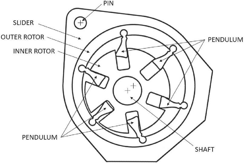
Figure 1 Schematic two-dimensional example of pendulum slider pump architecture.
2 Methodology
This work presents a validation of the numerical simulation of a pendulum slider pump. In this section, both the experimental and numerical setups used for the investigation are presented and discussed.
2.1 Experimental Test Bench
The case study consists of a pendulum slider pump characterized by a maximum displacement of 79 cm/rev and 7 pendulums. Its main components are the same as the example shown in Figure 1. The machine is designed to operate in the revolution frequency range 1000 rpm – 3000 rpm at temperatures of 30C – 180C. The pump of interest has been experimentally analysed by means of a test rig suitable for steady-state testing of a similar variable displacement pump. The hydraulic fluid adopted for the experimental campaign is a synthetic transmission oil for commercial vehicles, characterized by the properties listed in Table 1.
Table 1 Main properties at 40C and 100C of the oil of interest
| Temperature [C] | Kinematic Viscosity [mm/s] | Density [kg/m] |
| 40 | 51.1 | 841 |
| 100 | 9.3 | 801 |
2.1.1 Test bench description
The test rig used for experiments can be represented by means of the hydraulic scheme shown in Figure 2. The main components are:
C: displacement control mechanism; D: orifice; EM: electric motor; F: KRAL OMG 52 flowmeter (KRAL GmbH, Lustenau, Austria); H: heater; M: Kistler 4503B050WP0B1KA1 torque sensor (Kistler Group, Winterthur, Switzerland); P: pendulum slider pump under test; PI: Kulite XTL-123G-190 pressure transducer (rated absolute pressure: 1.7 bar) (Kulite Semiconductor Products, Inc., Leonia, NJ); PO,PP: Kulite XTL-123G-190 pressure transducers (rated absolute pressure: 17 bar) (Kulite Semiconductor Products, Inc., Leonia, NJ); R: reservoir; T: PT100 class B resistance temperature detector; VO: outlet valve; VP: pilot solenoid valve.
Referring to the scheme shown in Figure 2, the pump under test P is powered by the electric motor EM, mechanically connected to the drive shaft of P through a torque sensor M with encoder. The latter is used to measure the torque and the revolution frequency of the shaft. The pump is accommodated in a moulded aluminium housing that connects it to the hydraulic system of the test rig. The housing is sealed towards the environment by a cover, and it lodges the displacement control mechanism C as well.
Focusing on C, it could be described as composed of the pivoting slider of the pump, pinned in the housing, and a spring that tends to force the slider against a mechanical stop in maximum displacement position. As represented by the cylinder scheme in Figure 2, the outlet pressure acts on a portion of the external surface of the slider, creating a force that tends to promote displacement reduction by rotating the stator. Moreover, another part of that surface is exposed to the pressure of a pilot chamber, resulting in an additional force opposed to the one due to the outlet pressure.
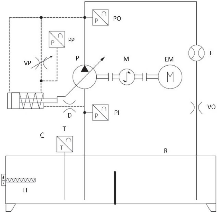
Figure 2 Hydraulic scheme of the test rig of interest according to ISO.
In the end, the rotational equilibrium between fluid forces and the spring force on the slider sets the position of the latter and, therefore, the displacement. In particular, the pilot chamber draws fluid from the delivery line by means of the solenoid valve VP, which can be adjusted to modify the pressure drop through it to tune the control mechanism. The same chamber discharges fluid to the suction through the gaps of the pump, represented by orifice D. Two dedicated transducers, PI and PO, are placed, respectively, at the inlet and the outlet of the pump to measure the pressure at those locations. The pressure transducer PP monitors the pilot chamber.
Regarding the main line of the circuit, the pump draws fluid from a reservoir R with flooded suction, the temperature of which is conditioned by heater H and measured by the resistance temperature detector T. A unique delivery duct leads the fluid back to the reservoir, passing through the flowmeter F, which measures the delivery volumetric flowrate, and the outlet valve VO, which sets the characteristic flow-pressure curve of the circuit.
2.1.2 Test matrix description
The pump under test has been analysed by considering two sets of stationary speed-control operating points at constant revolution frequency settings. As summarized in Table 2, equally-spaced levels every 500 rpm in the range 1000 rpm – 2500 rpm at approximate isothermal conditions at 40C have been tested for each set.
Table 2 Test matrix of the presented experimental campaign at 40C, reporting the studied revolution frequency levels
| Displacement Control | Level 1 [rpm] | Level 2 [rpm] | Level 3 [rpm] | Level 4 [rpm] |
| Variable | 1000 | 1500 | 2000 | 2500 |
| Fixed | 1000 | 1500 | 2000 | 2500 |
In particular, it has been decided to analyse two different scenarios in terms of displacement control (“variable” and “fixed”). For the first set, a finite spring precharge force has been adopted. For the second one, it has been decided to disable the displacement control mechanism by applying an extremely high precharge load, as it tended to infinity. The idea is to force the pump to operate at fixed maximum displacement, independently of the forces exerted by the hydraulic fluid. The goal of this approach is to compare the behaviour of the machine at the analysed revolution frequency levels in the two different control scenarios, variable displacement and fixed displacement.
It has been decided to use a unique supply current setting of the solenoid valve VP for each run, independently of the considered set. Each operating point has been replicated three times, and the test matrix has been sequentially carried out in random order to minimize systematic errors.
The main quantities of interest are the average values of delivery volumetric flowrate, reservoir temperature, revolution frequency, and absolute inlet/outlet/pilot pressure as measured, respectively, by F, T, M, and PI/PO/PP. They are calculated basing on the signals recorded during acquisition periods of 10 s by the adopted data acquisition system imc CRONOSflex (imc Test & Measurement GmbH, Berlin, Germany). Regarding the hypothesis of isothermal conditions, runs that present reservoir temperature values in the range 38C – 42C during the whole acquisition period are deemed acceptable.
2.2 Numerical Set-up
While the fundamental physical equations governing the fluid dynamics remain the same, improvements made in numerical algorithms, physical models, grid generation technology, computer power, and software engineering technology have significantly increased the productivity and accuracy of new generation CFD software, especially when solving more complex problems.
Simerics-MP+ solves first principle conservation equations coupled with advanced physical models to provide accurate predictions of flow, pressure, and cavitation in pumps in a short turnaround time. In the following section, technical details of the code will be presented, focusing on key components that directly contribute to productivity and accuracy. The program packs all four key functions of the CFD process, i.e., grid generation, pre-processing, problem solution, and post-processing, into a single product [14].
2.2.1 Grid generation
The first step in translating a pump prototype into a CFD model is to create a numerical mesh of the geometry that will be used to discretize and solve the governing fluid dynamics equations. Pumps typically have very complex shapes, with curved surfaces and small gaps. Grid generation is the most labour-intensive part of a pump simulation process for most CFD packages [14]. Solution accuracy, speed, and convergence are all directly related to the quantity and quality of the grid cells. Given that grid generation is one of the deciding factors of CFD productivity and accuracy, the choice of the grid is a very important issue.
SimericsMP+ uses a proprietary meshing algorithm, the Conformal Adaptative Binary-tree (CAB) algorithm. CAB generates cartesian hexahedra cells in a volume enclosed by a group of “Water tight” surfaces. Close to the boundary, CAB will automatically adjust the grid shape to conform to the surfaces and critical geometry edges. In order to fit critical geometrical features, CAB will automatically adjust the cell size by progressive division of the mesh cells in half (binary grid). Body-fitted binary tree meshing is a flexible means of generating a highly efficient grid. This type of mesh belongs to a family of unstructured body-fitted Cartesian grids. This is the method used for static domains by the model discussed in this paper. Under this technique, an overlaid cubic grid is refined by factors of two as it approaches regions requiring higher geometric resolution. At a boundary, cells are cut to conform to the surfaces defining the fluid domain. This grid is accurate and efficient because:
• the parent-child tree architecture allows for an expandable data structure with reduced memory storage;
• binary refinement is optimal for transitioning between different length scales and resolutions within the pump;
• the majority of cells are cubes, which is the optimum cell type in terms of orthogonality, aspect ratio, and skewness thereby reducing the influence of numerical errors and improving speed and accuracy;
• it can be automated, greatly reducing the set-up time;
• since the grid is created from a volume, it can tolerate “dirty” CAD surfaces with small cracks and overlaps.
Regarding simulation accuracy for integrated values (like pressure head or flowrate) it has been found that binary tree meshes are as good as well-built boundary layer structured grids [14].
2.2.2 Governing equations and turbulence model
The fundamental equations to be solved (numerically) by any CFD code are the conservation of mass, momentum, and energy. Considering a control volume that is moving through time as part of a finite volume approach, the conservation equations of mass and momentum can be written, respectively, in their basic integral representation (without external source terms) as
in which
– is the control volume,
– is the control volume surface,
– is the surface normal pointed outwards,
– is the fluid density,
– is the fluid pressure,
– is the body force vector,
– is the fluid velocity vector,
– is the surface motion velocity vector.
, the shear stress tensor, is a function of the fluid viscosity and the velocity gradient. For a Newtonian fluid, it is given by the following equation:
where is the unit tensor of second order.
The software implements mature turbulence models, such as the standard k model and RNG k model [15]. These models were available for more than a decade and were widely demonstrated to provide good engineering results. The standard k model, used for the simulations presented in this paper, is based on the following two equations applied to a moving control volume:
with , , , ; here e are the turbulent kinetic energy and the turbulent kinetic energy dissipation rate Prandtl numbers, respectively. The turbulent kinetic energy and its dissipation rate are defined as:
in which the strain tensor ( and ) is expressed as:
where and are components of the turbulent fluctuation velocity, and and are components of the spatial vector. The turbulent viscosity and the turbulent generation term are calculated by:
where , is a component of , and is the Reynolds stress; the latter is a component of the Reynolds stress tensor , which can be modelled through the Boussinesq hypothesis:
2.2.3 Real liquid property model
In past CFD simulations, analysts used to treat liquid as an incompressible fluid with constant density. As a matter of fact, the average liquid density can change due to cavitation, aeration, and liquid compressibility. Cavitation refers to the formation of vapor bubbles from the primary liquid when the pressure drops below vapor pressure, subsequently followed by bubble collapse at regions where the pressure rises again above vapor pressure. Aeration refers to the presence of non-condensable gases in the primary liquid, such as air in water. Although the amount is typically small, liquid can also be highly compressed depending on the pressure level. In some cases, assuming the fluid as being incompressible is indeed a reasonable approximation, but, in other cases, cavitation, aeration, and liquid compressibility must be considered to capture important physics, otherwise one will end up with incorrect results [14].
At low inlet pressure, cavitation and/or aeration bubbles can emerge, grow, and dramatically reduce pump performance. For positive displacement pumps, cavitation will cause losses in volumetric efficiency [16]. Without an accurate cavitation/aeration model, such efficiency losses cannot be calculated.
Gas and liquid mixtures are inherently difficult to simulate, due to the large density difference between the two phases and the strong coupling between the gas or vapor void fraction and the mean flow pressure.
The cavitation model implemented in the presented code takes all three important real liquid properties, cavitation, aeration, and liquid compressibility into account. This model is based on the work of [17], which has been implemented with several significant enhancements and improvements, such as, among others, the capability to account for distributions of dissolved air content, free air in form of dispersed gas bubbles, and the related release/dissolution phenomena [18]. Regarding the presented simulations, it has been chosen arbitrarily to adopt the simplest option implemented in the software environment, dealing with aeration by considering a constant free gas mass fraction of 10 as uniformly dispersed in the fluid to simplify the modelling effort.
2.2.4 Positive displacement pumps methodology
In setting up and running a model, Simerics-MP+ provides templates for a range of pumps, valves, and motors. These templates guide the set-up of a particular component type and control the mesh generation, based on the component’s inherent features. A template is used to create a structured looking mesh in the dynamic fluid volume, while static volumes (like ports, for example) are meshed using the Body-fitted binary tree methodology explained above. Tolerances and mesh size, globally and locally, can be then adjusted manually and refinement zones can be created where needed. The dynamic mesh cell count and topology are maintained during the simulation. Volume change is accommodated using a combination of mesh compression/expansion. Also in this case, tolerances can be then adjusted manually. This combination of template and automated meshing allows the simulation to include the geometry needed to conform to the real system.
2.2.5 Pendulum pump methodology
The pendulum pump described in this paper is, by all means, a positive displacement pump. Simerics-MP+, however, does not yet provide a ready-made template for this type of architecture. A specific procedure to handle the motion of the dynamic volumes, based on the principles explained in the previous sections, has been then developed, and schematically reported in Figure 3. The starting point is a set of annulus segment volumes (Figure 3(a)), discretised with a structured hexahedral grid, positioned with respect to a reference direction in the plane perpendicular to the revolution axis. These volumes are then morphed by projection/rejection functions based on the actual pendulum and rotors geometries (Figure 3(b)); these geometries are imported into the code as sets of points. The volumes position and shape are updated at each timestep as the rotors turn and the pendulums swing around their hinge point integral with the outer rotor.
The pendulum pump methodology has been implemented into Simerics-MP+ via a set of scripts developed in the Simerics Expression Language and some lookup tables which provide geometry profiles and weighting functions for the mesh deformation. It has been applied to the pendulum slider design addressed in this paper, in combination with the Body-fitted binary tree approach for static volumes, but it is a general methodology that can be applied to different pendulum-like positive displacement devices, and it will be integrated into the main code as a template in a future software release.
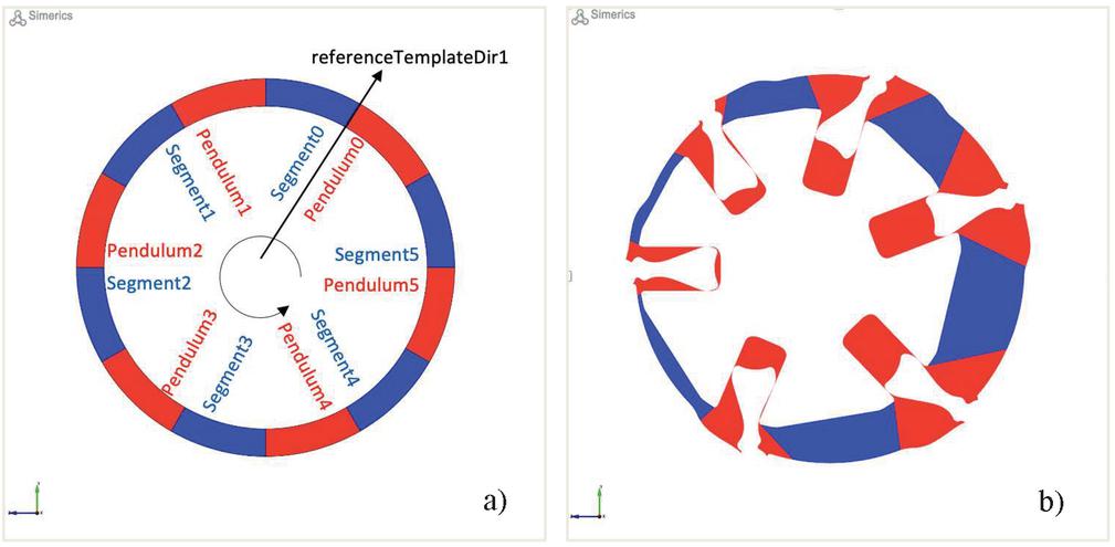
Figure 3 Rationale for grid generation of a representative pendulum slider pump: a schematic of the pumping chambers initial hexahedral grid (a) and the respective morphed representation (b).
2.2.6 Dynamic equation for ring motion
Concerning the simulation of the mechanism that allows displacement variation in the pendulum slider pump of interest, the rigid body theory can be applied to determine the rotational motion of the stator ring around its pin, quantified by the ring angle . Considering the proposed approach, the following Ordinary Differential Equation (ODE) based on the balance of angular momentum is solved at run-time by the dedicated ODE Simerics-MP+ solver [19]:
where is the moment of inertia of the ring around the pin centre, and are, respectively, the torque due to the pressure force and the spring force, and is an additional torque due to other forces acting on the ring. The coupled solution procedure consists of the following steps.
1. Start with an initial position of the ring (maximum displacement) which defines the outer rotor position.
2. The fluid equations are solved.
3. The forces acting on the fluid-solid interfaces around the ring are then computed as the input for the angular momentum equation.
4. The ODE is integrated over time to obtain the new position of the ring for the new time step.
5. A re-meshing step is carried out based on the new position of the ring.
2.2.7 Determination of the forces acting on the ring for the pendulum pump
For the pendulum pump considered in this project, is calculated basing on the force contributions on the ring due to the external chambers (inlet domain, outlet domain and pilot chamber), as depicted in Figure 4, and is derived by the characteristics of stiffness and precharge of the spring under the assumption of linear behaviour.
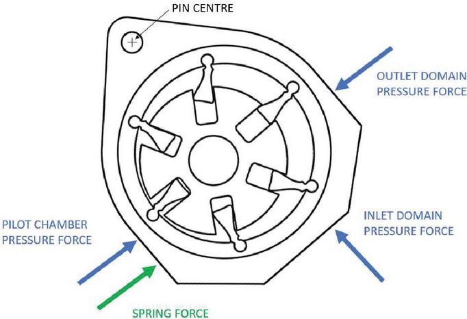
Figure 4 Schematic of the external forces acting on the ring.
The torque due to internal forces, such as the ones transmitted to the outer rotor (and, then, to the ring) by the pendulums and the pressure on its internal surface, should then be considered as additional torque in the ring dynamic equation described above. The calculation of that contribution is currently being implemented, so it has not been possible to use it to simulate the pump of interest in variable displacement conditions yet.
3 Results
3.1 Experimental Results
The main outputs of the experimental campaign are reported in Figure 5 in terms of average values of delivery volumetric flowrate (), outlet pressure (), inlet pressure (), and pilot pressure as functions of the average revolution frequency. In particular, the mean values of the displayed quantities over the three replicates are shown, as well as the respective type-A 95 % confidence uncertainty intervals based on Student’s t-distribution. As it can be deduced from Figure 5, the experimental dispersion of replicated runs could be deemed negligible.
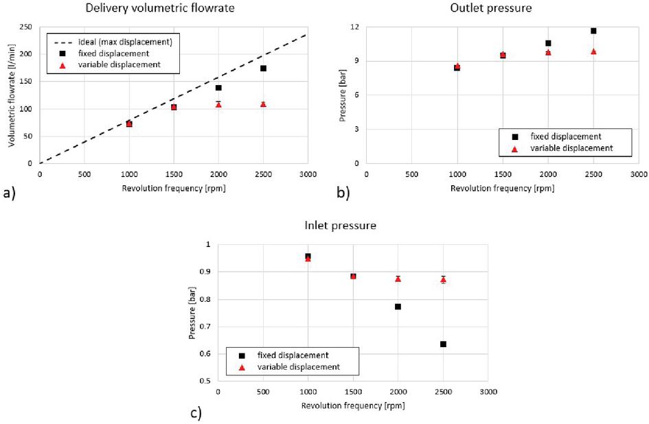
Figure 5 Experimental results in terms of average values of delivery volumetric flowrate (a), absolute outlet pressure (b), and absolute inlet suction pressure (c) as functions of the average revolution frequency for both the analysed control scenarios; the respective type-A error bands are reported.
Referring to the datasheet [20] of the adopted pressure transducers for each full scale of interest, it has been decided to neglect the type-B error bands of the measured pressure values. Typical values of combined error band of non-linearity, hysteresis and repeatability (0.1 % FS), thermal zero shift (0.01 % FS/F), and thermal sensitivity drift (0.01 %/F) are declared by the manufacturer. Uncertainties lower than 0.1 bar, for PP and PO, and 0.01 bar, for PI, result from the propagation of the cited error sources by means of the root-sum-square rule under the assumption of uncorrelated inputs [21]. Type-B error bands of flowrate values have been neglected as well, in light of the accuracy of 0.1 % of the measured value that results from the flowmeter datasheet [22].
Moreover, some relevant derived quantities are reported in Figure 6 against the average revolution frequency. In particular, the average pump pressure difference and the average hydraulic power are displayed, as defined in the following equations.
They represent the pressure load of the pump and the power output of the machine, respectively. Moreover, the picture reports also the experimental results in terms of hydraulic power ratio , as defined in the following equation.
Here and are the average hydraulic power of the variable displacement and the fixed displacement scenarios, respectively, both assessed at the same operating point in terms of revolution frequency setting. Their ratio represents the difference in terms of power output between the two considered control scenarios at the same revolution frequency level. In particular, the mean values of the derived quantities over the three replicates are shown in Figure 6, as well as the respective type-A 95 % confidence uncertainty intervals like the ones of Figure 5.
3.1.1 Fixed displacement behaviour
Analysing the fixed displacement behaviour, it can be noticed that in Figure 5(a) the pump presents a flowrate profile that is quite close to the ideal one for the pump at maximum displacement, calculated as the maximum displacement times the revolution frequency. It shows increasing volumetric losses as the revolution frequency and the outlet pressure, as depicted in Figure 5(b), are increased. On the contrary, the inlet pressure presents the decreasing trend shown in Figure 5(c), as plausibly expected. The related pump pressure difference values result in an almost linearly increasing behaviour up to approximately 11 bar, as shown in Figure 6(a), leading to hydraulic power outputs up to about 3.2 kW, as depicted in Figure 6(b).
The trends are meaningful for a fixed displacement machine, but it is difficult to understand if the cited volumetric losses are entirely due to internal leakage, or if some small displacement reductions have occurred. In fact, it should be noted that small eccentricity variations might have been possible, because of the finite stiffness of the mechanical constraint of the control spring. For the sake of completeness, it should be stated that the pilot chamber is flooded with oil during tests, even if the control mechanism is disabled. In fact, absolute pilot pressures in the range (6–9) bar have been measured. In this sense, a portion of the leakage could have been due to the recirculating flow from the outlet to the pilot chamber, and then back to the inlet through internal gaps of the pump.
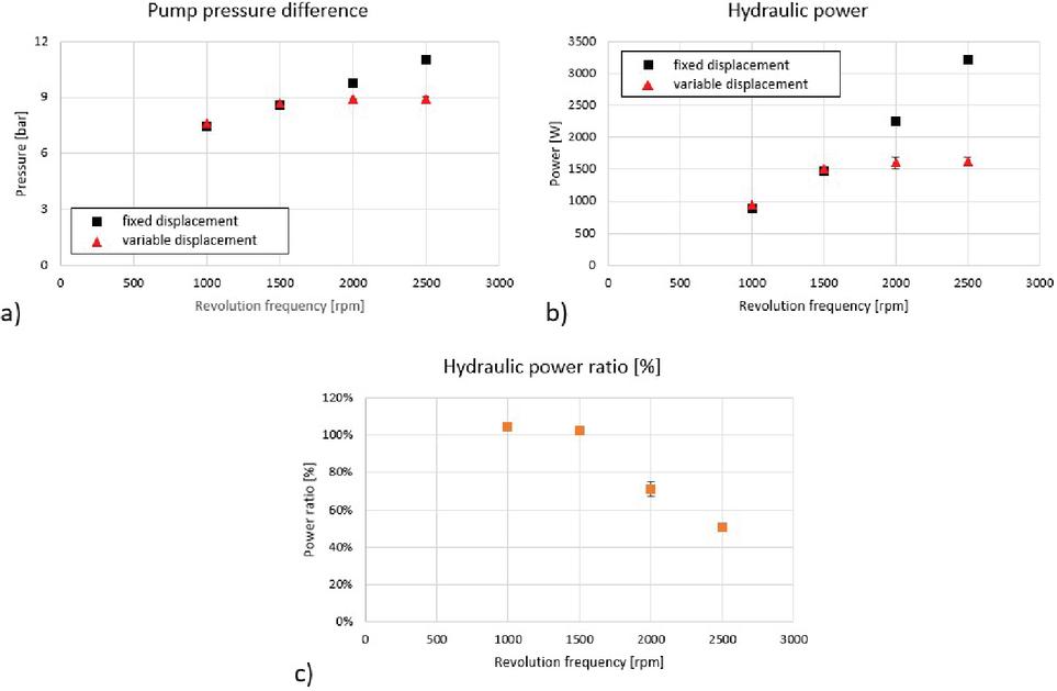
Figure 6 Experimental derived quantities in terms of average values of pump pressure difference (a) and hydraulic power (b), both as functions of the average revolution frequency for the two analysed control scenarios, and hydraulic power ratio (c) against the average revolution frequency; the respective type-A error bands are reported.
3.1.2 Variable displacement behaviour
Regarding the behaviour of the pump in case of variable displacement conditions, Figure 5(a) shows flowrate results in line with the ones of the fixed displacement behaviour up to 1500 rpm, suggesting that the machine has been operating at maximum displacement at those conditions. The trends of the rest of the output quantities shown in Figure 5 seem to confirm this hypothesis. As additional confirmation, the resultant hydraulic power ratio is close to 100 % at those revolution speed settings.
On the contrary, considering the data points at 2000 rpm and 2500 rpm in Figure 5(a), the flowrate increases just slightly as the revolution frequency increases, leading to the almost flat inlet pressure profile shown in Figure 5(c). The marked difference between the flowrate trends in the two different displacement control cases is a symptom that significant displacement reductions have occurred at revolution frequencies over 1500 rpm. Moreover, Figure 5(b) shows the tendency of the system to limit the absolute outlet pressure at about 10 bar, which is the threshold at which displacement reductions have taken effect for the chosen control settings. In fact, the absolute outlet pressure trend results to be just slightly increasing in the range (1500 – 2500) rpm as the revolution frequency is increased, leading to a maximum pump pressure difference of about 9 bar, as shown in Figure 6(a).
The consequence of the enabled control mechanism is a maximum hydraulic power of about 1.6 kW, reached at the maximum addressed revolution frequency as shown in Figure 6(b). The respective hydraulic power ratio in Figure 6(c) depicts approximately a 50 % reduction of the maximum output of the machine.
3.2 Numerical Results
3.2.1 Fixed displacement behaviour
A set of simulations has been performed to validate the behaviour of the pump when no displacement variations are admitted. For this purpose, four operating points have been chosen: 1000 rpm, 1500 rpm, 2000 rpm, and 2500 rpm. Two of them, 1000 rpm and 1500 rpm, represent conditions at which no experimental evidence of spontaneous displacement variations has been found, independently of the status of the displacement control mechanism. The remaining two, 2000 rpm and 2500 rpm, has shown the contrary during experiments; they represent conditions at which the machine would exhibit significant displacement changes if they were admitted.
For all the analyses presented here, a constant axial gap has been applied, in accordance with the measured clearances of the tested pump. The fluid was modelled as a compressible oil with the same characteristics (density, bulk modulus, saturation pressure) as the one used in the experiments. An almost negligible presence of non-condensable gas was considered as dispersed in the liquid, as requested by the SimericsMP+ real liquid model.
The 1000 rpm results in terms of average delivery volumetric flowrate against the crank angle are reported in Figure 7, which clearly shows the ripple related to the pendulum passage (7 pendulums). A total oscillation of around the 10 % of the flowrate is obtained, and the average value is remarkably close to the experiments, leading to 72.7 l/min against an experimental value of 72.4 l/min.

Figure 7 Delivery flowrate against the crank angle resulting from the 1000 rpm numerical analysis.
Very similar flowrate patterns are obtained for all the other operating points, and the respective average values are plotted in Figure 8 along with the ideal and experimental results derived from Figure 5(a). The agreement is very good and below 5 % for all points except for the 2500 rpm case, showing a satisfying overall model performance. Even though a similar deflection on experimental results could be considered acceptable from the common industry standards, further investigations are required to understand the reason of the discrepancy at the highest speed. For all cases, little to no cavitation is experienced inside the investigated fluid domains.
3.2.2 Variable displacement behaviour
As explained in Section 2.2.7, it has not been possible to apply the dynamic equation for the ring to the pendulum pump model. However, to test the functionality, it has been decided to run the model at fixed revolution frequency and variable eccentricity values (by varying the rotation angle of the pivoting ring around its pin, simulation by simulation) to capture the flowrate variability as the displacement of the virtual machine is reduced. The focus is on the revolution frequency conditions where experimental evidence of spontaneous eccentricity variations has been found.
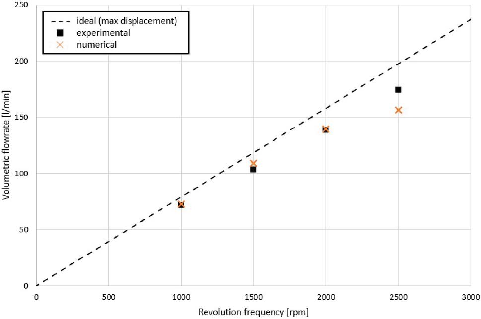
Figure 8 Comparison of numerical and experimental results in terms of average delivery volumetric flowrate against the average revolution frequency for the fixed displacement scenario; the ideal volumetric flowrate at maximum displacement conditions is reported.
The results are shown in Figure 9, where the non-dimensional flowrates at 2000 and 2500 rpm, defined as the predicted average delivery volumetric flowrate divided by the one at the maximum eccentricity for the considered revolution frequency level, are plotted versus the ring angle of rotation. An abscissa equal to zero indicates the maximum displacement position. The model runs smoothly and reliably as the eccentricity changes, showing decreasing trends of the flowrate as a function of the rotation angle.
With reference to Figure 9, it is conceptually possible to find the value of abscissa at which the predicted flowrate matches the respective experimental variable-displacement result of Figure 5(a) at each considered revolution frequency level. Assuming that the machine has been running approximately at constant eccentricity at those operating points, that approach could be used to estimate the average displacement at which the pump is supposed to operate at those conditions, in order to distinguish the effects of volumetric losses and displacement variation on the flowrate.
It should be noted that the accuracy of the trends of Figure 9 is difficult to assess, since, aside from the maximum eccentricity condition, no other experimental tests at known fixed intermediate displacement have been carried out for reference. Nevertheless, the analysis shows the feasibility of using the model to investigate eccentricity scenarios that are different from the maximum displacement condition, with the purpose to study any case in which the machine can be assumed to operate approximately at constant eccentricity.
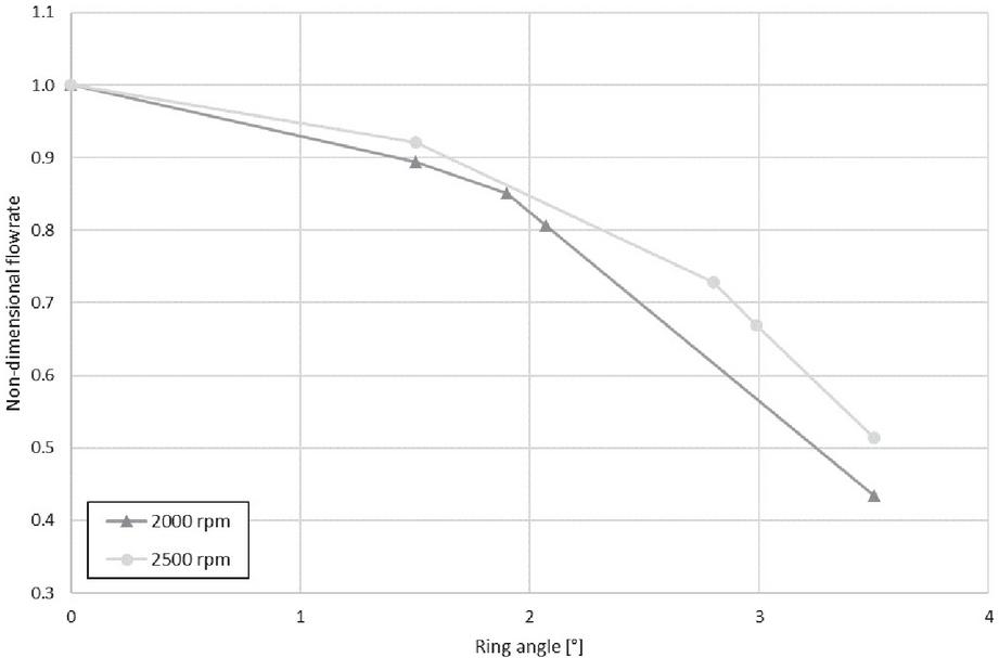
Figure 9 Variation of the predicted non-dimensional flowrate as a function of the ring angle at 2000 rpm and 2500 rpm.
4 Summary and Conclusion
In this paper, the framework for analysing a pendulum slider pump with the CFD software suite Simerics-MP+ has been developed. The procedure has been applied to a 7-pendulums pump with a maximum displacement of 79 cm/rev, experimentally tested at the ZF Automotive Italia Srl. plant in San Giovanni di Ostellato (Italy). An ad-hoc equipment that allows the machine to vary its displacement during tests or not, starting from the maximum eccentricity condition, has been used.
The CFD model has been developed both for fixed and variable displacement scenarios, even though the force balance for the dynamic equilibrium of the stator has not been implemented yet. Regarding the maximum eccentricity operating points, very good agreement with the experiments has been found at almost all the rotational speeds, while some discrepancies have been found for the highest value. This might be related to uncertainties about oil behaviour in terms of aeration which can affect the filling of the pumping chambers of the simulated machine, especially at high speed.
Regarding the simulations of fixed intermediate displacement conditions, additional experimental tests are needed to assess the accuracy of the results. The work proves nevertheless the feasibility of the proposed approach to study displacement conditions different from the maximum.
Besides these aspects to be further investigated, the developed model has shown a very good behaviour in terms of robustness and accuracy, in line with Simerics-MP+ standards, and it candidates to be released soon in an official version. Despite the described limitations, the overcoming of which is the natural next step of this work, it is believed that the addressed numerical approach constitutes a valuable opportunity for analysts to get an insight into the behaviour of variable displacement pendulum machines from a three-dimensional perspective. Considering the state of the art, it is an achievement that could be deemed precious for the CFD community.
Acknowledgements
It is desired to thank Mr. Giovanni Novi and Mr. Mauro Ardizzoni of the Test&Validation Department of the ZF Automotive Italia S. r. l. plant in San Giovanni di Ostellato (Italy) for their technical support on the experimental campaign, Dr. Ettore Fadiga for the helpful suggestion, Mr. Laurent Mitri and Mrs. Miriam Crepaldi of University of Ferrara and Rudi Niedenthal of SIMERICS GmbH in Rottenburg (Germany) for their technical support on the numerical implementation and campaign.
Nomenclature
| Variable | Description | Unit |
| Turbulence model coefficient | [–] | |
| Turbulence model coefficient | [–] | |
| Turbulence model coefficient | [–] | |
| Body force | [N/m] | |
| Turbulence generation | [kg/(m s)] | |
| Full scale | [Pa] | |
| Index | [–] | |
| Moment of inertia | [kg m] | |
| Outward-pointing surface normal | [–] | |
| Turbulent kinetic energy | [m/s] | |
| Pressure | [Pa] | |
| Average hydraulic power | [W] | |
| Average hydraulic power of the fixed displacement scenario | [W] | |
| Average hydraulic power of the variable displacement scenario | [W] | |
| Average inlet pressure | [Pa] | |
| Average outlet pressure | [Pa] | |
| Average delivery volumetric flowrate | [m/s] | |
| Reynolds stress tensor | [Pa] | |
| Hydraulic power ratio | [–] | |
| Strain tensor | [1/s] | |
| Time | [s] | |
| Pressure torque | [N m] | |
| Spring torque | [N m] | |
| Additional torque | [N m] | |
| Turbulent fluctuation velocity component | [m/s] | |
| Velocity component | [m/s] | |
| Spatial vector component | [m] | |
| Velocity | [m/s] | |
| Surface velocity | [m/s] | |
| Unit tensor of second order | [–] | |
| Turbulent kinetic energy dissipation rate | [m/s] | |
| Ring angle | [rad] | |
| Viscosity | [Pa s] | |
| Turbulent viscosity | [Pa s] | |
| Density | [kg/m] | |
| Control volume surface | [m] | |
| Turbulent kinetic energy dissipation rate Prandtl number | [–] | |
| Turbulent kinetic energy Prandtl number | [–] | |
| Shear stress tensor | [Pa] | |
| Reynolds stress | [Pa] | |
| Average pump pressure difference | [Pa] | |
| Control volume | [m] |
| Acronym | Description |
| Computational Fluid Dynamics | |
| Positive Displacement Machine | |
| Ordinary Differential Equation |
References
[1] Rundo, M., Nervegna, N., Lubrication pumps for internal combustion engines: a review, International Journal of Fluid Power, Vol. 16, No. 2, pp. 59–74, 2015.
[2] Jensen, H., Janssen, M., Beez, G., Cooper, A., Potential fuel savings of the controlled pendulum-slider pump, MTZ worldwide, Vol. 71, No. 2, pp. 26–30, 2010.
[3] Conrad, H., Knauß, R., Controlled pendulum-slider oil pump for the supply on demand of transmissions, ATZ worldwide eMagazine, Vol. 113, No. 12, pp. 34–41, 2011.
[4] Conrad, H., Janssen, M., Combined oil-vacuum pump, MTZ worldwide, Vol. 76, No. 7, pp. 8–13, 2015.
[5] Schopp, J., Düngen, R., Wetzel, M., Spieß, T., The V8 Gasoline Engine for the New 7-Series BMW, MTZ worldwide, Vol. 76, No. 9, pp. 34–41, 2015.
[6] Hannibal, W., Kirsch, B., Bode, B., Hausner, S., Efficiency measurements of oil pumps under the influence of air content, MTZ worldwide, Vol. 79, No. 10, pp. 50-53, 2018.
[7] Vrolix, A. S. T.,Pompe à alluchons oscillants, Patent FR980766A, 1951.
[8] Beez, G., Bauer, H.G., Lademann, S., Adjustable pendulum slide valve machine, Patent DE4434430A1,1996.
[9] Beez, G., Bauer, H.G., Lademann, S., Pump or hydraulic motor with inner and outer rotors, Patent DE19532703C1,1996.
[10] Wanninger, H., Pump and hydrodynamic retarder equipped with said pump and gear unit equipped with such a pump, Patent US20150129363A1, 2015.
[11] Kovacevic, A., Stosic, N., Smith, I., Screw compressors: three dimensional computational fluid dynamics and solid fluid interaction (Vol. 46). Springer Science & Business Media, 2007.
[12] Suman, A., Ziviani, D., Gabrielloni, J., Pinelli, M., De Paepe, M., Van Den Broek, M., Different numerical approaches for the analysis of a single screw expander. Energy Procedia, 101, 750–757, 2016.
[13] Morini, M., Pavan, C., Pinelli, M., Romito, E., Suman, A., Analysis of a scroll machine for micro ORC applications by means of a RE/CFD methodology. Applied Thermal Engineering, 80, 132–140, 2015.
[14] Ding, H., Visser, F. C., Jiang, Y., Furmanczyk, M., Demonstration and Validation of a 3D CFD Simulation Tool Predicting Pump Performance and Cavitation for Industrial Applications, FEDSM2009-78256, Volume 1: Symposia, Parts A, B and C, pp. 277–293; 2009.
[15] Yakhot, V., Orszag, S.A., Thangam, S., Gatski, T.B. & Speziale, C.G., Development of turbulence models for shear flows by a double expansion technique, Physics of Fluids A, Vol. 4, No. 7, pp. 1510–1520, 1992.
[16] Jiang, Y., Furmanczyk, M., Lowry, S., Zhang, D., Perng, C. Y.. A three-dimensional design tool for crescent oil pumps (No. 2008-01-0003). SAE Technical Paper, 2008.
[17] Singhal, A. K., Athavale, M. M., Li, H., Jiang, Y., Mathematical basis and validation of the full cavitation model. J. Fluids Eng., 124(3), 617–624, 2002.
[18] Stuppioni, U., Suman, A., Pinelli, M., Blum, A., Computational Fluid Dynamics Modeling of Gaseous Cavitation in Lubricating Vane Pumps: An Approach Based on Dimensional Analysis. J. Fluids Eng., Vol. 142, p. 071206, 2020.
[19] Wang, D. M., Ding, H.; Jiang, Y.; Xiang, X., Numerical Modeling of Vane Oil Pump with Variable Displacement, SAE Technical Paper Series, SAE International, 2012.
[20] Kulite Semiconductor Products, Inc.. Ruggedized automotive pressure transducers. XTL-123G-190 (M) SERIES. On the https://kulite.com//assets/media/2021/08/XTL-123G-190.pdf, Accessed: 09/18/2021.
[21] Coleman, H. W., Steele, W. G., Experimentation, validation, and uncertainty analysis for engineers. John Wiley & Sons, 2018.
[22] KRAL GmbH. Flow Measurement. On the https://www.kral.at/fileadmin/data/files/products/KRAL/\_Flowmeters\_Display\_and\_Processing\_Unit.pdf, Accessed: 09/18/2021.
Biographies
Umberto Stuppioni received the M.Sc. in Mechanical Engineering from University ofFerrara in 2019. As of September 2022, he is enrolled as Ph.D. student at the same university, and he works as CAE Specialist at ZF Automotive Italia S.r.l., Italy. His research areas include design, simulation, and testing of fluid power systems.
Nicola Casari received a bachelor’s degree in mechanical engineering from the University of Ferrara in 2013, a master’s degree in mechanical engineering from the University of Ferrara in 2015, and the philosophy of doctorate degree in Engineering Science from the University of Ferrara in 2019, respectively. He is currently working as a Research Fellow at the Department of Engineering, University of Ferrara. His research areas include aeroacoustics and multiphase flows.
Federico Monterosso received his Sciences degree in Aeronautical Engineering from the University of Rome “La Sapienza” in 1990. He worked as a Research Assistant at the Imperial College of London and then at Computational Dynamics (now part of Siemens Software), AEA Technology (now part of Ansys Inc.) and Enginsoft Spa. In 2007, he co-founded OMIQ srl, an engineering company based in Milan, Italy focused on the application of CFD technology to turbomachinery and hydraulics applications. Since his graduation, he’s been involved in the development of Computational Fluid Dynamics tools and their implementation in the industrial environment.
Alessandro Blum received the M.Sc. in Mechanical Engineering from University of Padua in 2014. He achieved the Ph.D. in Mechanical Engineering, issued by University of Ferrara, in 2021. As of September 2022, he works as Head of Engineering Department atAutomotive Italia S.r.l., Italy. His managerial role concerns product development of fluid power systems in the automotive field.
Davide Gambetti received the M.Sc. in Mechanical Engineering from University of Ferrara in 2005. As of September 2022, he works at ZF Automotive Italia S.r.l., Italy, where he serves as Senior Project Engineer. He has held that product development role since 2005, gaining significant experience in the field of automotive fluid power systems.
Michele Pinelli graduated in Mechanical Engineering at the University of Bologna in 1997, where he obtained the title of PhD in 2001. Since 2021 he has been Full Professor of Fluid Machines at the Engineering Department of the University of Ferrara. From 2018 to 2021 he was Pro-Rector Delegate to the Third Mission of the University of Ferrara. His research activity is documented by more than 240 scientific articles published mainly in international journals and international congresses. He is the scientific director of several international research collaborations, including Imperial College London and St. John’s College of the University of Oxford.
Alessio Suman is a researcher at University of Ferrara. He holds a B.S. and M.S. in Mechanical Engineering from University of Ferrara. Dr. Suman attended the Engineering Science PhD course at the University of Ferrara where he worked on the performance degradation of gas turbine. In addition, he was involved in a numerical simulation of energy systems and volumetric displacement machine. He has authored numerous publication about energy systems and turbomachinery related topics. His main research interests include the design of experimental test and the numerical simulation of positive displacement machines.
International Journal of Fluid Power, Vol. 24_2, 299–326.
doi: 10.13052/ijfp1439-9776.2426
© 2023 River Publishers