Numerical Simulation of a Spool Valve in Gaseous Cavitation Conditions
Emma Frosina1,*, Gianluca Marinaro2, Amedeo Amoresano2 and Adolfo Senatore2
1Department of Engineering, University of Sannio, Benevento, Italy
2Department of Industrial Engineering, University of Naples “Federico II” Naples, Italy
E-mail: frosina@unisannio.it; gianluca.marinaro@unina.it; amedeo.amoresano@unina.it; senatore@unina.it
*Corresponding Author
Received 09 June 2022; Accepted 21 July 2022; Publication 29 September 2022
Abstract
Spool valves are subject to a deteriorated performance and noise due to the occurrence of cavitation phenomena. It is well known that cavitation effects the performance of the component and causes an unwanted noise. The noise sound levels are influenced by many parameters like geometries and opening areas. In this paper a simple valve body made in plexiglass has been tested analyzing the cavitating area in U-grooves. A dedicated test rig has been equipped with a high-speed camera to acquire images of the phenomenon. A numerical three-dimensional CFD model has been built up using the commercial code. Experimental imagines have been compared with the numerical results showing a high accuracy on the prediction of the gaseous cavitation. The numerical results allow separate examination of several distinctive flow characteristics, which show favorable consistency with experimental observation and a periodic evolution of cavitation structure.
Keywords: Gaseous cavitation, spool valve, 3D – CFD numerical approach, experimental tests.
Nomenclature
| Acronym | Description | |
| CAD | Computer-Aided Design | |
| CFD | Computational Fluid Dynamic | |
| EDGM | Equilibrium Dissolved Gas Model | |
| EFD | Experimental Fluid Dynamics | |
| NCG | Noncondensable gas | |
| Symbol | Description | Unit |
| Cavitation condensation coefficient | [] | |
| Cavitation evaporation coefficient | [] | |
| D | Diffusivity of the vapor mass fraction | [m/s] |
| Diffusivity of the dissolved NCG | [m/s] | |
| f | Mass fraction of free NCG | [] |
| Mass fraction of dissolved NCG | [] | |
| Equilibrium gas mass fraction of dissolved NCG | [] | |
| Equilibrium mass fraction of the dissolved NCG at the reference pressure | [] | |
| Mass fraction of the vapor | [] | |
| Kinematic flow gradient | [] | |
| Turbulent kinetic energy | [J/kg] | |
| Surface normal | [] | |
| Total noncondensable gas mass fraction | [] | |
| Pressure | [Pa] | |
| Inlet Pressure level | [Pa] | |
| Reference pressure for the dissolved gas equilibrium mass fraction. | [Pa] | |
| Outlet pressure level | [Pa] | |
| Phase-change threshold pressure | [Pa] | |
| Radius to pressure relief groove | [m] | |
| R | Vapor generation rate | [] |
| R | Vapor condensation rate | [] |
| Source of dissolved NCG | [kg/m] | |
| Temperature | [K] | |
| Fluid velocity vector | [m/s] | |
| Fluid velocity vector | [m/s] | |
| Greek letter | Description | Unit |
| Turbulent viscosity | [Pas] | |
| Density of mixture | [kg/m] | |
| Density of gas | [kg/m] | |
| Density of liquid | [kg/m] | |
| Density of vapor | [kg/m] | |
| Surface of control volume | [m] | |
| Control volume | [m] | |
| Turbulent Schmidt number | [] |
1 Introduction
It is known that the fluid control is one of the most important function of the hydraulic system and the hydraulic valves are the preset elements to set pressure, regulate or direct a flow [1].
Nowadays, spool valves are the most common valves to direct a flow; directional control valves are utilized in many applications and fields (industrial, mobile, marine, etc.) and their performance are, usually, evaluated in terms of pressure drop, operating limits, switching times, power consumption, etc. However, in some particular application the noise generated by those components becomes crucial. Gaseous cavitation (aeration or pseudo-cavitation) is in fact a source of noise.
Many studies have been focused on the improvement of the proportional valve performance focusing the attention on the fluid bourse noise. Cavitation areas are usually located in the grooves (U-grooves, V-grooves) that connects the ports each other’s. As said, there are two major problems accompanied with occurrence of cavitation one is related to the noise one to the deterioration of the component’s performance.
Analysis on the sound levels and the noise spectrums helps on the investigation on the cavitation beginning [1].
Martin et al. [2] presented a study on spool valves with an experimental investigation to look at the cavitation in aircraft hydraulic systems. The purpose of the investigation was to identify mechanisms which lead to damage. The test facility, used by authors, allowed the measurement of parameters in order to identify non-cavitating and cavitating conditions.
Oshima et al. [3–6] studied experimentally the cavitation phenomenon in two poppet valves. Authors demonstrated that the geometry mostly effects on the cavitation onset, noise and induced choking phenomenon in the flow rate characteristics.
In this paper the cavitation in a spool valve is analyzed using experimental tests, the results of numerical simulations obtained using a 3D CFD methodology will be shown in the next paragraphs. The comparison between data will be presented with a high accuracy of the numerical model that could help for the understanding of the cavitation location and for supporting the designer to avoid this phenomenon.
2 Experimental Setup
An open center directional valve (shown in Figure 1a) has been analyzed in this paper. The valve body of a geometry already on the market has been redesigned in plexiglass to be easily accessible via highspeed-camera. The areas of interest are located in the spool grooves and will be later described.
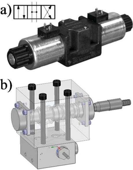
Figure 1 Valve under investigation.
The dedicated test rig has been used for this research; the layout is shown in Figure 2. Two pressure transducers (AVL LP11DA) to measure the upstream/downstream pressure of the valve have been placed in the manifold clearly shown in Figure 1b. The transducer located at the inlet port has a measuring range of 0–30 bar while the second (outlet port) has a measuring range 0–5 bar. The spool position has been manually controlled by a micrometer, also shown in Figure 1b.
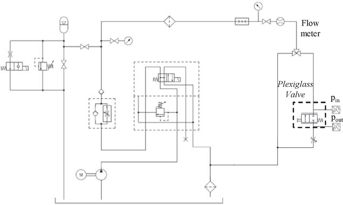
Figure 2 Test ring layout.
The plexiglass model in Figure 1b consists of two ports, a body and a spool (in Figure 3a). The spool is moved inside the valve body thought the micrometer in Figure 3b; in this way it is possible to measure with a good accuracy its position and, consequently, act on the metering area. The generation of a gaseous cavitation has been observed for spool stroke of 2 mm therefore, for this spool position, experiment have been done using a high-speed camera. The high-speed camera is a FastCam Mini AX100 and has been placed in front of the valve, looking at the area of interest, shown in Figure 3a. The camera delivers 1-megapixel image resolution (1024 1024 pixels) at frame rates up to 4,000 fps.
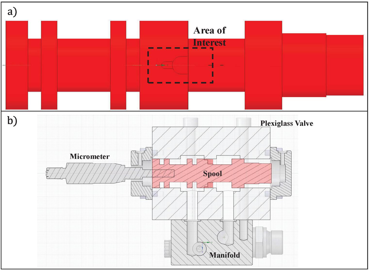
Figure 3 Spool valve – Area of interest.
A first pictures is shown in Figure 4 where, for the same spool opening stroke of 2 mm, two working condition have been analyzed, one with a delta pressure between the ports of 2 bar (on the left) and 18 bar (on the right) respectively. Looking at Figure 4b the bubbles are clear and defined while when the delta pressure is low, like in Figure 4a, there is a complete absence of the cavitation phenomenon.
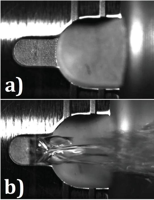
Figure 4 Comparison between two working condition for a spool stroke of 2 mm.
The next paragraph is dedicated to the description of the numerical methodology used to study the gaseous cavitation phenomenon.
3 Numerical Model Description
The gaseous cavitation phenomenon in the U-groove of the valve under investigation has been also investigated using Simerics MP+ (developed by Simerics Inc.), a 3D CFD code that solves the fundamental conservation equations of mass, momentum and energy. The model includes also accurate physical models for turbulence and cavitation.
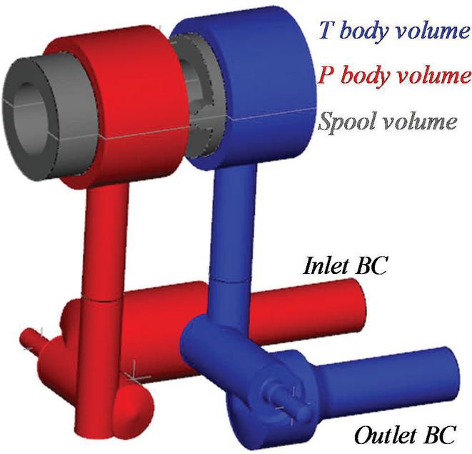
Figure 5 Valve extracted fluid volume.
The extracted valve fluid volume is shown in Figure 5 where ports T and P are respectively of the low and high pressure; in figure also the spool volume and the boundary condition surfaces are highlighted. The extracted fluid volumes have been meshed using the grid generator of Simerics MP+ that is based on body-fitted binary tree algorithm. The meshed volume is shown in Figure 6. while in Figure 7 the refinement zone applied.
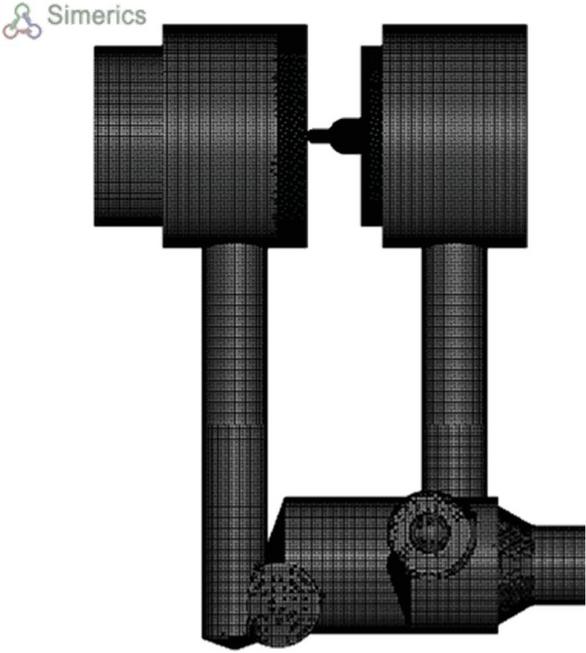
Figure 6 Valve fluid volume: Mesh.
A mesh sensitivity analysis has been done increasing and decreasing the cells number in the area of interest. In Figure 7a comparison between a model of 1.4 million of cells (Figure 7a) and the final model (Figure 7b); that consists of 3 million of elements. Other models with finer mesh have been analyzed and compared with the model in Figure 7b; however, those simulations required supplementary time with almost the same numerical results. For this reason, the model in Figure 7b has been chosen for this analysis.
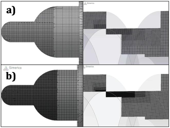
Figure 7 Mesh refinement in the U-groove: comparison between a model of 1.4M cells and a model of 3M cells.
The code includes many cavitation models to predict the cavitation, aeration and liquid compressibility. In this paper the Equilibrium Dissolved Gas Model (EDGM) for cavitation has been selected; this model is based on the work of Singhal [8], based on Navier-Stockes equations for variable fluid density and the Rayleigh-Plesset equation.
The original cavitation model proposed by Singhal et al. describes the vapor distribution using the following formulation:
| (1) |
Where D is the diffusivity of the vapor mass fraction and is the turbulent Schmidt number. In the present study, these two numbers are set equal to the mixture viscosity and unity, respectively. The vapor generation term, R, and the condensation rate, R, are modeled as:
| (2) | |
| (3) |
The Singhal’s cavitation theory includes the mass fraction of Non-Condensable Gas (NCG) in the liquid. The variable mixture (liquid, liquid vapor and NCG) density is calculated in according to the Equation (4):
| (4) |
The NCG in the hydraulic fluid can be found as a free and a dissolved state. The free NCG mass fraction f has not been considered constant, but its evaluation has been achieved adding an additional transport equation of the gas (5).
| (5) |
Where the equilibrium gas mass fraction depending on the current cell pressure, has been evaluated by the following equation:
| (6) |
Hereby, the sum of free gas mass fraction and dissolved gas mass fraction is constant:
| (7) |
Under these equations, only one equation has been solved for the dissolved gas ; the free gas is subsequently solved based on the being constant [9].
Numerical simulations have been run in the same working condition of the experimental tests. The boundary conditions are listed below:
• Total pressure at inlet that varies in the range [1–18] bar abs;
• Static pressure at outlet of 1 bar abs;
• The fluid is a Hydraulic oil ISO VG46;
• Variable dynamic viscosity;
• Variable liquid bulk modulus (linearly dependent with pressure);
• Dissolved air 4% vol;
• Undissolved air 0.1% vol;
• Temperature 318 K.
The model does not include heat transfer; therefore, the temperature is assumed to affect the oil viscosity and density. The “standard k-” turbulence module has been used to predict the effective turbulent viscosity [7–10].
Simulations have been run on an Intel(R) Core (TM) i7-7700HQ CPU 2.80 GHz 16 cores, with a computational time of around 20 minutes per simulation; it is important to underline that the convergence criteria for the flow is of 10 while for the turbulence and cavitation is of 10.
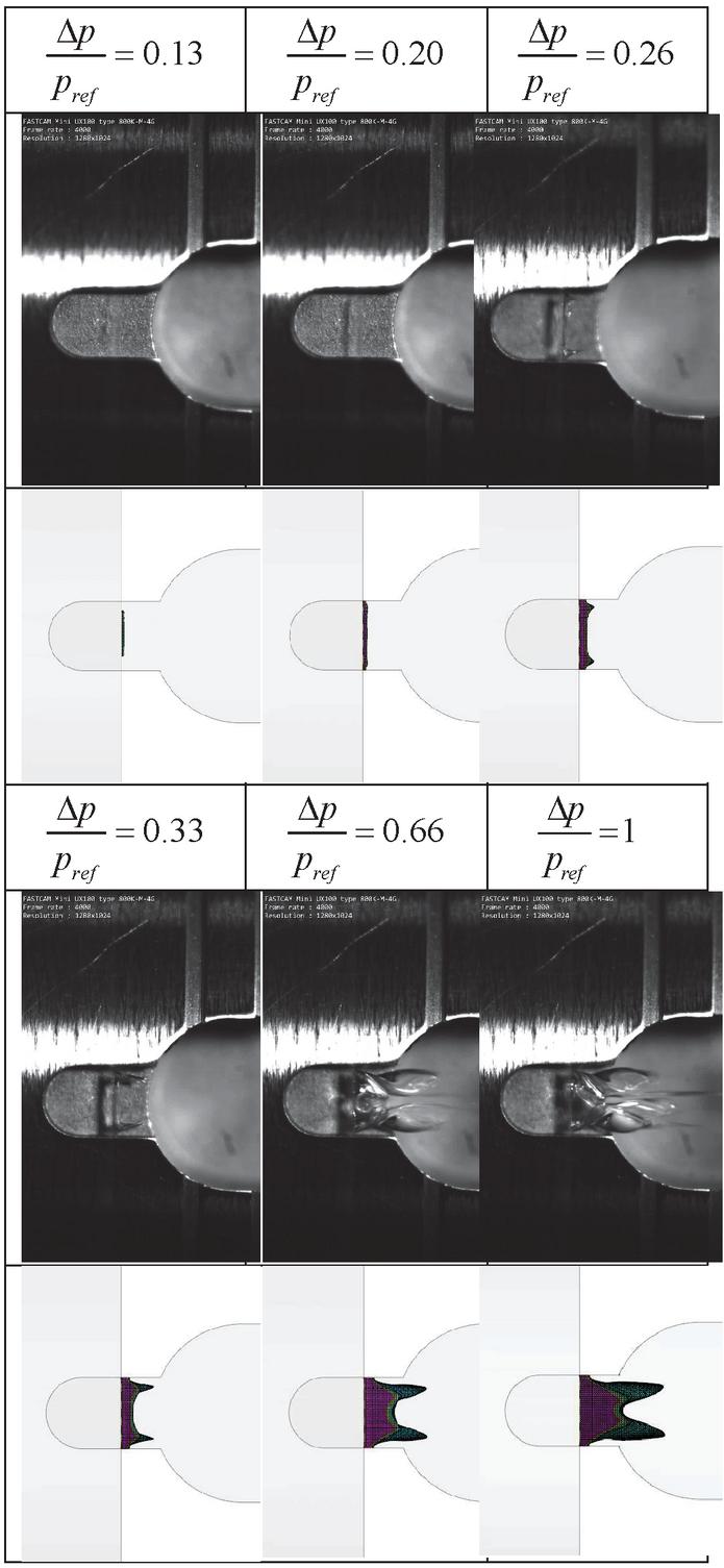
Figure 8 Numerical model results and experimental data comparison.
4 Results and Discussion
The model, as said, has been run varying the pressure at the inlet side of the port P. The experimental data and simulated results have been compared and showed in Figure 8 for each analyzed working condition. Figure 8 shows, for some working conditions, the experimental pictures on the top and the modelled ones on the bottom.
Analyzing results in Figure 8, it is clear that the model is able to predict the cavitation phenomenon with a high accuracy, confirming that the proposed methodology can help the understanding of the cavitation location and can support the designer to avoid this unwanted phenomenon. The next steps of this research will explore other valve opening and will regard the post-processing of the experimental pictures in order to better compare the bubble contouring.
5 Conclusions and Future Developments
In this paper an open center directional spool valve has been studied using both a CFD and an EFD approaches with the main proposal of identify gaseous cavitation for a first reference spool geometry with U-groove. First of all, a simple valve body, made in plexiglass (PMMA), has been manufactured and tested using a high-speed camera. The camera delivers 1-megapixel image resolution (1024 1024 pixels) at frame rates up to 4,000fps. Several working conditions have been tested by changing the inlet pressure of the valve in the range [1–18] bar abs. Then, using the commercial code Simerics MP, an accurate numerical three-dimensional CFD model of the valve has been built up. The model includes the Equilibrium Dissolved Gas Model (EDGM) cavitation model to predict the cavitation, aeration and liquid compressibility. Experimental imagines have been compared with the numerical results showing a high accuracy on the prediction of the gaseous cavitation; therefore, as said, the proposed methodology can help for the understanding of the cavitation location and can support the designer to avoid this phenomenon.
Results presented in this paper are only a part of the ongoing research activity that is focused on the study of the fluid bourn noise due to the cavitation. Thus, noise and vibration have been acquired as well.
Funding
Results presented in this paper are part of a PhD program supported by the Italian Government and the MIUR (Ministry of Education, Universities and Research).
Acknowledgments
The authors thank Simerics Inc., for providing them a license. They also acknowledge Federico Monterosso and Micaela Olivetti of OMIQ srl, Michele Pavanetto of Duplomatic MS and Gennaro Stingo and Giuseppe Iovino of University of Naples.
References
[1] X. Fu, L. Lu, X.D. Ruan, J. Zou, X.W. Du, 2008, Noise Properties in Spool Valves with Cavitating Flow, International Conference on Intelligent Robotics and Applications ICIRA 2008: Intelligent Robotics and Applications pp. 1241–1249;
[2] C.S. Martin, H. Medlarz, D. C. Wiggert, C. Brennen, 1981, Cavitation inception in spool valves, J. Fluids Eng., 103(4), pp. 564–575;
[3] S. Oshima, T. Ichikawa, 1985, Cavitation Phenomena and Performance of Oil Hydraulic Poppet Valve: 1st report mechanism of generation of cavitation and flow performance. Bulletin of JSME, 28(244), pp. 2264–2271.
[4] S. Oshima, T. Ichikawa, 1985, Cavitation Phenomena and Performance of Oil Hydraulic Poppet Valve: 2nd Report, Influence of the Chamfer Length of the Seat and the Flow Performance. Bulletin of JSME, 28(244), pp. 2272–2279.
[5] S. Oshima, T. Ichikawa, 1986, Cavitation Phenomena and Performance of Oil Hydraulic Poppet Valve: 3rd report, influence of the poppet angle and oil temperature on the flow performance. Bulletin of JSME, 29(249), pp. 743–750.
[6] S. Oshima, T. Leino, M. Linjama, K. T. Koskinen, M. J. Vilenius, 2001, Effect of cavitation in water hydraulic poppet valves., International Journal of Fluid Power, 2(3), pp. 5–13.
[7] E. Frosina, A. Senatore, D. Buono, K. A. Stelson, 2016, A Mathematical Model to Analyze the Torque Caused by Fluid–Solid Interaction on a Hydraulic Valve, J. Fluids Eng., 138(6): 061103;
[8] A.K. Singhal, M.M. Athavale, H.Y. Li, Y. Jiang, 2002,“Mathematical basis and validation of the full cavitation model, J. Fluids Eng. vol. 124, pp. 617–624.
[9] E. Frosina, G. Marinaro, A. Senatore, M. Pavanetto, Effects of PCFV and Pre-Compression Groove on the Flow Ripple Reduction in Axial Piston Pumps, Proceeding of 2018 Global Fluid Power Society PhD Symposium, GFPS 2018; Samara; Russian Federation; 18–20 July 2018.
[10] Inc. S. Simerics MP’s User Manual – v 5.0.11.
Biographies

Emma Frosina is an Assistant Professor at the Department of Engineering of the University of Sannio Benevento. She received her M.S. Degree in Mechanical Engineering from the University of Naples Federico II in 2012 and her Ph.D. Degree in Mechanical Systems Engineering in 2016. She is the author of over 50 scientific papers published in peer-reviewed international journals and in international conference proceedings. Her research interests are in the fluid power field where she is mainly specialized in modeling and optimization of components (machines, valves, etc.) using numerical approaches (both lumped parameter and three-dimensional CFD) and testing.

Gianluca Marinaro is a Research Engineer at CIRA (Italian Aerospace Research Centre). He is committed to the numerical modeling and design of propulsive architecture for the aeronautical sector. From 2016 to 2021, he was involved in Fluid Power Research, getting his Ph.D. at the University of Naples Federico II in 2020, working in both academic and industrial sectors. His research interest was in the design optimization of hydraulic pumps and valves by means of numerical modeling in both 0D and 3D environment and in prototype development and testing.

Amedeo Amoresano is currently an Associate Professor in the Department of Industrial Engineering (DII), Università degli Studi di Napoli Federico II. He received the M.S. Degree in Mechanical Engineering from Università degli Studi di Napoli Federico II in 1991 and the Ph.D. Degree in Mechanical Systems Engineering in 1994. He is the author of over 100 scientific papers published in peer-reviewed international journals and in international conference proceedings, with an h-index of 16 and over 700 citations. His research interests include: concentrated solar power plants, trigeneration power plants, atomization and sprays, exhaust emissions and fuel consumption of SI engines fuelled with gasoline-ethanol blends, sulphur oxides abatement in exhaust gases, geothermal systems, instability of dynamic systems, hydraulics and pneumatic systems. His research and academic profile can be found at the following link:

Adolfo Senatore from 2000 is a Full Professor at the Department of Industrial Engineering of the University of Naples Federico II. Before, he was Associate Professor from 1996 to 2000 and Assistant Professor since 1995. He received the M.S. Degree in Mechanical Engineering from University of Naples Federico II in 1980. He is the author of over 300 scientific papers published in peer-reviewed international journals and in international conference proceedings. His research interests are in the fluid power and internal combustion engines fields where he is mainly specialized on modeling and optimization of components using numerical approaches and testing.
International Journal of Fluid Power, Vol. 23_3, 469–484.
doi: 10.13052/ijfp1439-9776.23311
© 2022 River Publishers