Path Planning and Smoothing for 4WDs Hydraulic Heavy-Duty Field Robots
Pekka Mäenpää* and Jouni Mattila
Faculty of Engineering and Natural Sciences, Tampere University, Tampere, Finland
E-mail: pekka.maenpaa@tuni.fi
*Corresponding Author
Received 09 June 2022; Accepted 21 July 2022; Publication 17 January 2023
Abstract
This paper discusses the path planning and path-following control for a four wheel drive (4WD), steer-articulated boom lift driven by hydraulic actuators. The environment is assumed to be both static and known. The path planning will be done in two phases, where the first one finds a crude, collision-free path accounting for the vehicle dimensions, and this path will be smoothed with a path smoothing algorithm to satisfy the kinematic and dynamic constraints imposed by the vehicle and its actuators. The path smoothing algorithm will be chosen from several candidates by using a simulated test scenario. Then, the simulation results will be used to verify the path planners feasibility in heavy-duty, four-wheel-steered field robots having hydraulic actuators and high inertia.
Keywords: Path planning, AI for hydraulic and pneumatic systems, efficient and intelligent fluid power systems.
Introduction
Path planning for autonomous ground vehicles is necessary for many real-world applications, and it is often intended to find these paths under holonomic constraints and in the presence of obstacles. However, the paths provided by many algorithms have unnecessary oscillations caused by either randomized trajectory segment sampling or by constraining these trajectories to a grid. Removing these oscillations is possible by increasing the discretization precision, but that is usually too computationally expensive to do globally. This is why the path planning is usually split into a crude path finding phase, which provides a drivable path but with severe oscillations, and a pathsmoothing phase, which can improve the existing path locally [1].
Both of these phases must generate trajectories between configurations. The trajectories must adhere to the vehicle constraints, which depend on the steering method. Most of the literature which considers path planning for ground vehicles with holonomic constraints focuses on car-like vehicles, but car-like and 4WS vehicles with similar steering angle limits have somewhat different requirements for executable trajectories. In addition to this, the vehicles are usually relatively light and have simple internal dynamics. 4WS vehicles can follow trajectories where the curvature is temporarily higher than in the minimum turning circle of the vehicle, and these vehicles can follow position trajectories with discontinuous curvature without stepwise changes in steering angles. Additionally, the heading of 4WS vehicles does not need to align with the trajectory tangent to follow its position accurately. However, the path following algorithms for 4WS vehicles usually include heading in the trajectories, and the heading is often aligned with the path.
The redundant degrees of freedom can be used to correct any lateral path following errors while simultaneously aligning the heading. Additionally, continuous path derivatives should improve trajectory following accuracy, because the actuator commands will be smoother.
The trajectories considered for these vehicles are usually at least cubic curves, because the cubic curves have enough degrees of freedom to generate trajectories with pose and curvature constraints at the end of the paths. For curves like these, solving the trajectory without exceeding a given maximum curvature is difficult, and methods such as [2] do not have analytical solutions. Using more degrees of freedom than this can make the trajectory design much simpler, but this can cause higher-order oscillations in the trajectory derivatives, because the higher-order derivatives are not constrained. Some path planning algorithms, like [3], ease this problem by using zero curvature values at the initial and final points of each spline trajectory, which does ensure curvature continuity, but the trajectories created by these algorithms cause some unnecessary actuation and the average curvature is not as high as the vehicle constraints would allow.
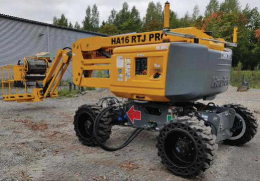
Figure 1 The simulated vehicle, Haulotte 16RTJ PRO.
The test robot modelled and simulated in this study is a boom lift Haulotte 16RTJ PRO in Figure 1. The rest of this study is organized as follows. The next section describes the architecture of the simulated system and its simulation model, the path following implementation, the path planning method and the path smoothing methods and differences between them. Section following that one describes the simulation results and the last section concludes the study.
System Architecture
The following sections describe the modelled robot and the path planning system architecture. Figure 2 describes the simulation system. The system is modelled using MATLAB Simulink with the Simscape Multibody environment. It is similar to [4], except for the changes in path planning. In the system, the path planner delivers poses along the path and a map describing the environment to the path smoother. The path smoother determines the appropriate maximum velocities v to use along the path and determines the control points for the trajectory generation. The trajectory generator then sends the desired position P, its derivative dP and the current maximum velocity v to the path – following controller. The path following controller determines the driving velocity v and heading commands for the robot. The driving velocity is the minimum of the current maximum velocity and the highest velocity possible with the current vehicle kinematics v, computed with the inverse kinematics. The inverse kinematics are also used to determine velocity v and steering commands for the actuator controller, which provides steering u and velocity u commands for the robot. The simulated robot then provides the current steering angle and velocity v commands used by the inverse kinematics. The ideal vehicle pose feedback (x, y, ) is computed based on the forward kinematics from the robot state.

Figure 2 The system structure used in simulation.
Modelled robot
The modelled robot is Haulotte 16RTJ PRO, a 4WD 4WS boom lift. The weight of the robot is 6650 kg, and it is powered by a hydraulic system, using a variable-displacement pump operating at a constant pressure of 150 bar. The pump is also connected to a pressure-controlled servo valve to improve its response times for rapid changes in required flow rates. Each wheel has its own hub motor controlled by a servo valve. The hub motors are fixed-displacement motors with attached travel reducers. The steering uses two independent symmetric hydraulic cylinders controlled by proportional valves, presented in Figure 3. Table 1 describes the vehicle dimensions.
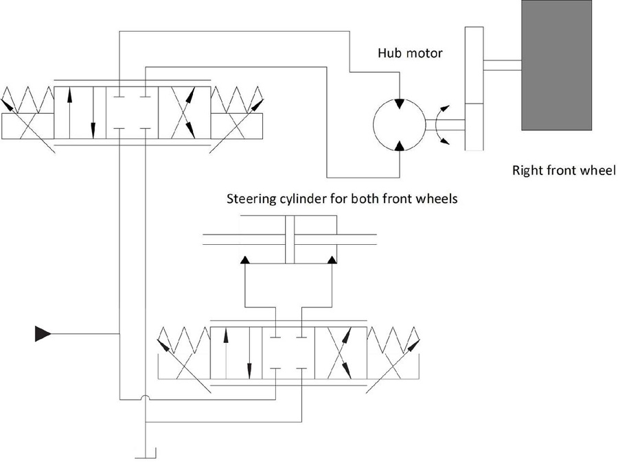
Figure 3 A simplified hydraulic diagram of the vehicle.
Table 1 Vehicle dimensions
| Dimensions | Value |
| Wheelbase (L) | 2.1 m |
| Dist. between wheel axle’s steering joints | 1.46 m |
| Dist. from steering joint to wheel center (c) | 0.24 m |
| Total length with boom stowed (el) | 6.75 m |
| Width (W) | 2.3 m |
Vehicle kinematics
The vehicle uses 4-wheel steering, which allows short turning radiuses for a robot of this size. The inverse kinematics describe the transformation from the velocities of the vehicle base frame {b} to steering angles and wheel velocities. The wheel frame {j} is offset from the steering joint frame {k}. Both the base frame and wheel frame velocities are described in terms of the world frame {w}.
| (1) | |
| (2) |
In these equations, the two-dimensional vector represents the translation between the frames. The steering angle command can be computed by using the arctangent of the velocity components of the steering joint frame {k}.
| (3) | |
| (4) |
All of these joints are modelled as rigid bodies using MATLAB Simulink and Simscape.
Hydraulics modelling
The hydraulic valves of the system are modelled as orifices as in [5], where the flow Q over the valve was computed as laminar or turbulent based on the nominal transient pressure p.
| (5) |
In these equations, K is a viscosity- and opening-dependent flow gain for the orifice.
| (6) |
The cylinders are modelled as fluid volumes where the pressure derivative is computed as a function of the effective bulk modulus of the volume B, total flow to the volume and time derivative of the cylinder volume V according to the following formula.
| (7) |
The modelled fixed-displacement motors have internal leakage linearly dependent on the pressure difference over the motor p and the leakage coefficient C, and the produced torque depends on the coulomb friction coefficient C, viscous friction coefficient C and rotation rate n in addition to the motor displacement V and pressure over the motor. The following formulas present the computation of flow to the motor and the momentum produced by the motor.
| (8) | |
| (9) |
The pump used in the system is modelled as a constant pressure source.
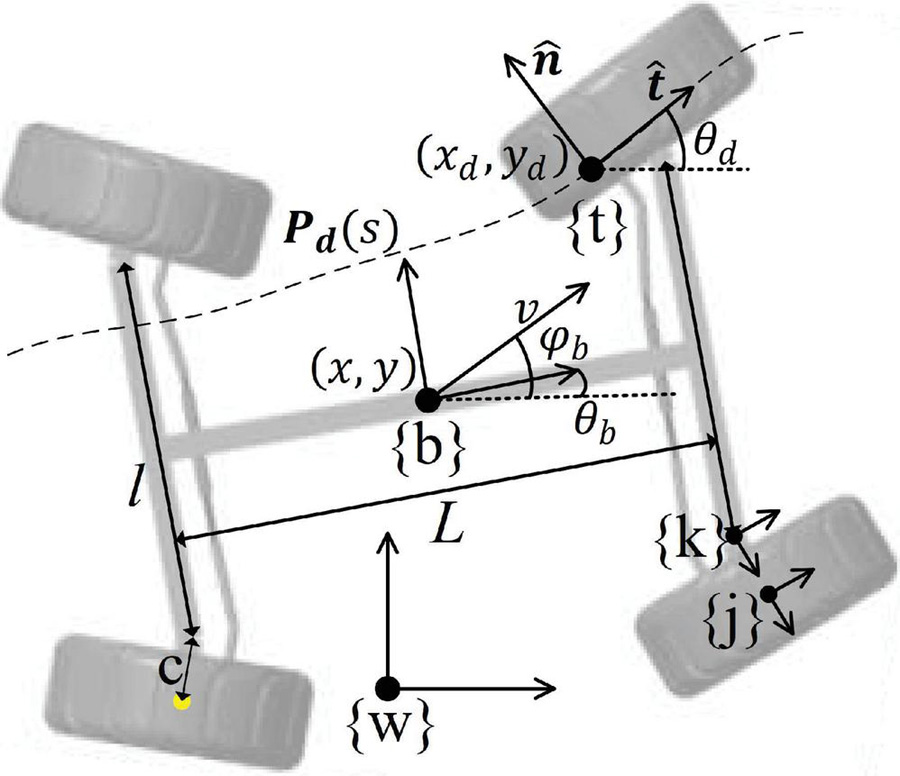
Figure 4 Coordinate frames used in modelling.
Path following algorithm overview
The path following algorithm is based on the controller introduced in [6]. The controller objective is to minimize the position and heading error between the pose provided by the path generator and the current vehicle frame {b}. The poses provided by the path generator are all tangent to the path. The steering type used by the controller is four wheel active steering, such as in [7]. With this steering type, the path follower can steer the front and rear wheels separately to improve path following precision.
Path planning
The path planning algorithm is based on [8], which finds a region covering the geometric path from the initial pose to the target pose. A set of poses from this region is sent to the path smoothing algorithm. For the purposes of path planning, the boom is assumed to be stowed, but without the jib tucked under. In this position, the length of the platform is much greater than its width, which is why the maneuver planning must be done in three dimensions. The exact dimensions of the used envelope are the vehicle dimensions el and W from Table 1. The search resolution in x-y-direction is adaptively improved as in a 2D search, but the heading range is discretized to 64 fixed slices. The heading is more reasonable to split with fixed discretization, because the same heading range can be used in all scenarios, whereas the position range can increase significantly. This allows the planner to compute the platform envelope for a small rotation range of /32 radians and to use it for each 2D slice as a fixed-orientation envelope. This makes finding the collision-free regions significantly simpler and computationally cheaper. Figure 5 presents the envelope based on vehicle dimensions and the envelope over the rotation range used in path planning. Because the path planning phase directly reports collision-free regions, the path smoothing phase could use these without requiring any collision checking. However, these collision-free regions tend to be so narrow that using collision checking separately in the path smoother allows it to find much smoother paths. Additionally, the planner reports the centres of each position and heading range as the poses in the path.
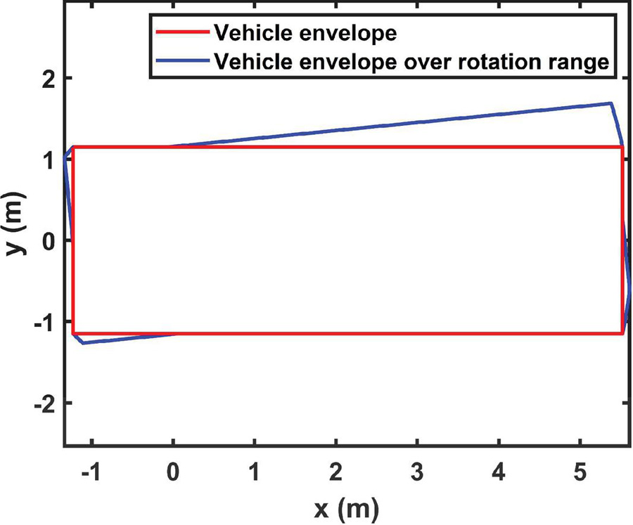
Figure 5 Envelope used in path planning.
Because the search is only 3-dimensional, the path planning could be done with a simple graph search based on a continuous-cost lattice, but increasing the discretization precision can be very beneficial with higher-dimensional workspaces. One such scenario is using a similar platform for a mobile manipulation task.
Path smoothing
The path smoothing works in two phases, where the first one attempts to shortcut the geometric path provided for smoothing, and the second one searches locally for an improved route. The shortcutting phase is free from local minima and can rapidly and significantly improve the path from the planner. The local search can reduce obstacle margins while retaining low curvature.
The local path search is based on the method used in [9], where the smoother samples points with a lateral offset from the original path. The algorithm then generates trajectories through these and the original points, creating a graph which is searched for the best available route. This process is repeated until the path search converges. Because this method uses discrete poses to define the path, the trajectories between the poses must be interpolated. The original algorithm used the curves generated by the method presented in [2], but these curves can not be analytically solved given the necessary constraints. This study used simpler Bezier curves, which have also the convex hull property, which states that the entire curve is inside the polygon defined by the control points, making correct collision checking simpler. The curvature continuity can be achieved by using Bezier curves, and the most commonly used cubic Bezier curves with 4 control points have enough degrees of freedom to solve the control point locations. However, the curvature at the endpoint of a Bezier curve depends on the three first control points of the curve, and a valid analytical solution may not exist at all. The solution can also be found by using a higher-order Bezier curve. This is why the poses were first connected with cubic Bezier curves, which were then elevated to quintic curves, and the curvature at the connection point of these curves was adjusted to match each other. The cubic curves can be elevated to quintic curves analytically, exactly and with a low computational cost. The curvature at the endpoints is matched by first enforcing G2-continuity and then scaling the control points according to the distances between the poses.
Because the platform is able to follow trajectories with curvature discontinuities, the paths with four-point Bezier curves were used as reference to compare the path following results. Additionally, the curvature at the connection point of two curves can be matched by either changing both curves to have the same curvature, creating a trajectory with lower derivatives, or by only changing the latter curve to match it with the former.
Using the former method would increase the complexity of the path planning significantly, or it must be applied to an existing trajectory. If it is applied to an existing trajectory, this alteration can lead to collisions, but the new trajectory can be collision-checked again and new collisions are unlikely as the position and heading changes are small. Additionally, with an iterative method like in [9], the trajectory can be adjusted after each search step, and the previous smoothing step can always be saved, which allows the path smoother to simply step back to an earlier iteration if the alteration leads to collisions.
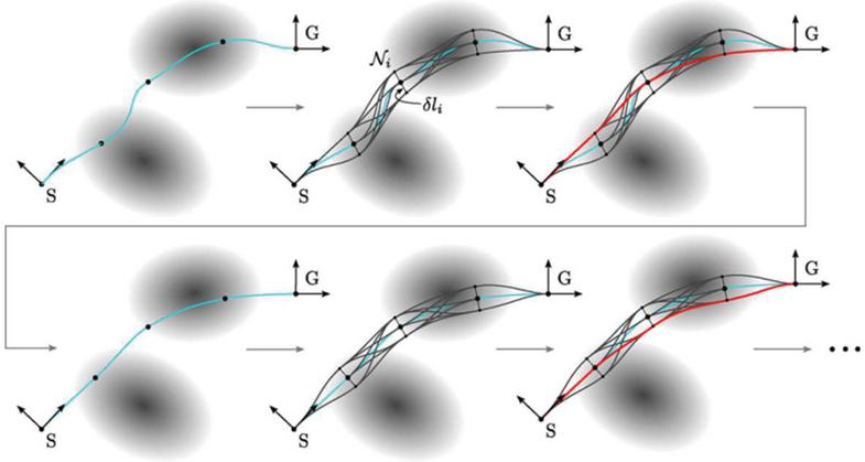
Figure 6 The smoothing method used in [9].
Figure 7 presents three alternative trajectories generated with the same three poses. The dashed line is a cubic Bezier curve. The control points of the curve following the pose i are defined as iPn, where the n signifies the index of the control point for the i:th Bezier curve. The control points are computed according to
| (10) | ||
| (11) | ||
| (12) | ||
| (13) |
where is the location of pose i, is the normalized orientation vector of pose i and d is the distance between the locations of poses i and i 1.
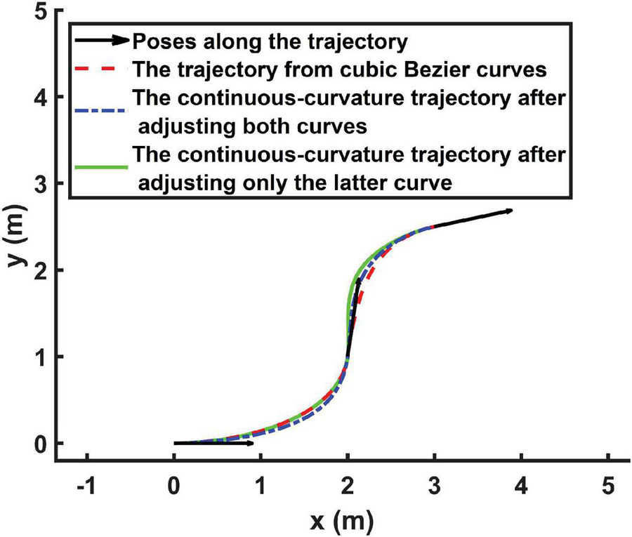
Figure 7 The trajectories generated based on the poses.
One of the main benefits of using Bezier curves is that the derivative function is easy to compute. The derivative curve D of a Bezier curve P defined by K 1 control points is a lower-order Bezier curve, and its control points can be computed as
| (14) |
where k must reach values 1 k K. The second and first derivatives of the Bezier curve at its first point are the first control points of the respective derivative curves, and based on this formula these derivatives only depend on the first three control points of the original curve. Because of this, the desired first derivative d1 at the start of a Bezier curve P can be set with the formula
| (15) |
and after this the second derivative d2 can be set with
| (16) |
The derivatives can be enforced similarly to the end of a curve by replacing Pi with PK 1 i in these formulas. If the derivatives are set to the same values, these formulas enforce G2 continuity. G2 continuity implies curvature continuity, because the curvature ct of a parametric curve can be computed with the first and second derivatives of the x- and y-components of the path with the following formula:
| (17) |
Because of this the demands for G2 continuity are stricter than for curvature continuity. Additionally, changing the first derivatives can drastically reshape the curves if these derivatives have significantly different magnitudes than the originals. This is why the first derivative should be scaled differently for both curves to match the original first derivatives. From the curvature formula, it is apparent that if the first derivative is scaled with a factor s and the second derivative must be scaled by s2, the curvature remains the same.
However, these formulas will change the first and last three control points of each curve. Matching the curvature for the last point of the curve should not effect the curvature at the first point of the curve, which is why the curves must be at least quintic 6-point curves.
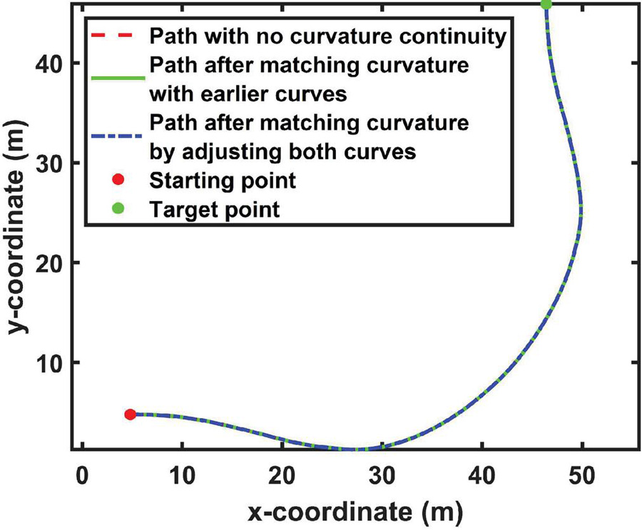
Figure 8 The followed path.
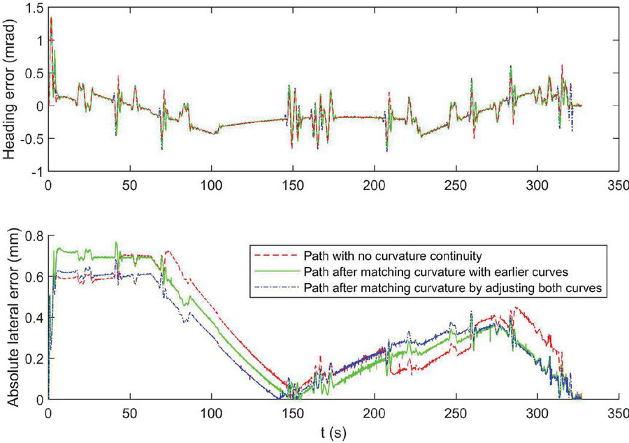
Figure 9 The lateral and angular path following errors.
The degree of a Bezier curve P can be elevated to create a one-degree higher curve Q without altering the curve shape. The first and last control points of Q must be the same as those of P, and the ones in between can be found by following the formula:
| (18) |
In the formula, the notation Q signifies the k:th control point of the curve Q, and the curve P is defined by K 1 control points. The indices of the control points start from zero, so that this formula must be applied for all of the indices 1 k K to find the complete curve Q. With this the cubic Bezier curves can be elevated to quintic curves and the curvature continuity can be guaranteed.
Simulation Results
The paths used in the simulation share the poses used between the trajectory segments, but the curvature matching between the segments is different, leading to different curvature values and slightly different paths.
Table 2 Path following errors. The best results are marked with .
| Lateral Error | Lateral Error | Angle Error | Angle Error | |
| RMS | Maximum | RMS | Maximum | |
| Path Type | (mm) | (mm) | (mrad) | (mrad) |
| Discontinuous curvature | 0.398 | 0.725 | 0.238 | 1.350 |
| Path after matching curvature | 0.394 | 0.768 | 0.242 | 1.350 |
| with earlier curves | ||||
| Path after matching curvature | 0.358 | 0.682 | 0.240 | 1.325 |
| by adjusting both curves |
The used methods are 4-point Bezier curves with discontinuous curvature, 6-point Bezier curves with continuous curvature matched by adjusting both curves and 6-point Bezier curves where the curvature is matched by only adjusting the curvature of the latter curve.
Figure 8 presents the reference paths used in the simulation. All of the paths were 79 meters long, and each consisted of 161 Bezier curves. The simulation results are gathered to Table 2. Adjusting two curves at a time to remove curvature discontinuities gives the best result as excepted, but removing the discontinuities by only adjusting the latter path does not produce better results than keeping the path unmodified. This is most likely caused by the higher curvatures in the adjusted path. In addition, all of the path following errors were small, below 0.8 mm for position and below 1.4 mrad for heading angle.
The lateral path following errors and angle errors over time are presented in Figure 9. The path angle errors are quite close to each other, and even the path with no curvature continuity has no clear jumps at the connection points of the curves. The lateral errors have clearer differences between the paths, but even then the RMS values are quite close to each other. This figure also shows that there is no significant differences in path following speed. All of the curves terminated near the same timestep with similar terminal accuracy. The path follower control target is reaching the target vehicle pose, which causes the path to have longitudinal error separately from the lateral error. This error was not plotted, because it has no effect on collisions in static environment.
Conclusions and Future Work
Constraining the path planning to continuous-curvature segments can severely limit the performance of many path planning algorithms, and the path curvature and distance from obstacles can be limited more reliably when the paths are not re-adjusted to correct these curvature discontinuities. The results strongly suggest that curvature continuity constraints are unnecessary for even heavy-duty 4WS vehicles, which allows the use of more efficient path planning and path smoothing algorithms.
As a future work, a similar system is intended to be used with planning for mobile manipulators, which has similar issues with the lack of research for heavy-duty manipulators, and which is also assumed to benefit significantly from the adaptive division of the configuration space.
References
[1] S. M. LaValle, Planning algorithms. Cambridge university press, 2006.
[2] B. Nagy and A. Kelly, “Trajectory generation for car-like robots using cubic curvature polynomials,” Field and Service Robots, vol. 11, 2001.
[3] X. Bu, H. Su, W. Zou, and P. Wang, “Curvature continuous path smoothing based on cubic bezier curves for car-like vehicles,” in 2015 IEEE International Conference on Robotics and Biomimetics (ROBIO), pp. 1453–1458, IEEE, 2015.
[4] H. Liikanen, M. M. Aref, R. Oftadeh, and J. Mattila, “Path-following controller for 4wds hydraulic heavy-duty field robots with nonlinear internal dynamics,” IFAC-PapersOnLine, vol. 52, no. 8, pp. 375–380, 2019.
[5] M. Hyvönen, J. Vilenius, A. Vuohijoki, and K. Huhtala, “Mathematical model of the valve controlled skid steered mobile machine,” in The 2nd International Conference on Computational Methods in Fluid Power Technology FPNI’06, August 2–3, 2006 Aalborg University, Denmark, 2006.
[6] R. Oftadeh, M. M. Aref, R. Ghabcheloo, and J. Mattila, “Bounded-velocity motion control of four wheel steered mobile robots,” in 2013 IEEE/ASME International Conference on Advanced Intelligent Mechatronics, pp. 255–260, July 2013.
[7] B. Li and F. Yu, “Optimal model following control of four-wheel active steering vehicle,” in 2009 International Conference on Information and Automation, pp. 881–886, IEEE, 2009.
[8] P. Mäenpää, M. Aref, and J. Mattila, “Formi: A fast holonomic path planning and obstacle representation method based on interval analysis,” in 2019 IEEE International Conference on Cybernetics and Intelligent Systems (CIS) and IEEE Conference on Robotics, Automation and Mechatronics (RAM), pp. 398–403, IEEE, 2019.
[9] P. Krüsi, P. Furgale, M. Bosse, and R. Siegwart, “Driving on point clouds: Motion planning, trajectory optimization, and terrain assessment in generic nonplanar environments,” Journal of Field Robotics, vol. 34, no. 5, pp. 940–984, 2017.
Biographies

Pekka Mäenpää Ph.D. student at Tampere University. Completed masters in Automation Technology 2021.

Jouni Mattila Dr. Tech. received his M.Sc. (Eng.) in 1995 and Dr. Tech. in 2000, both from the Tampere University of Technology (TUT), Tampere, Finland. He is currently a Professor of machine automation with the unit of Automation Technology and Mechanical Engineering, Tampere University. His research interests include machine automation, nonlinear model-based control of robotic manipulators and energy-efficient control of heavy-duty mobile manipulators.
International Journal of Fluid Power, Vol. 24_1, 59–76.
doi: 10.13052/ijfp1439-9776.2413
© 2023 River Publishers