Analysis of Frequency Adjustable Control of Permanent Magnet Synchronous Motor for Pump-controlled Actuators
Viacheslav Zakharov* and Tatiana Minav
IHA Innovative Hydraulics and Automation, Faculty of Engineering and Natural Sciences, Tampere University, Tampere, Finland
E-mail: viacheslav.zakharov@tuni.fi; tatiana.minav@tuni.fi
*Corresponding Author
Received 09 June 2022; Accepted 21 July 2022; Publication 17 January 2023
Abstract
Recently the pump-controlled system has actively been proposed as a replacement for conventional valve-controlled systems, to improve the energy efficiency in non-road mobile machinery. Earlier research demonstrated that a pump-controlled hydraulic system combines the best properties of traditional hydraulics and electric intelligence. This pump-controlled system can be realized via direct control of hydraulic pimp/motor by varying speed of electric motor without complex servo valves. Nowadays, a wide range of different electric motors is known and available with efficiency higher than 95% One of the most attractive option of electric motor is Permanent Magnet Synchronous Motor (PMSM) due to its size, power, and high efficiency.
However, control of electric motors in pump-controlled systems has are not yet considered and not well researched.
In this paper, the main objective of this investigation is determination of control values for the pump-controlled actuator and analysis of system’s behavior in different applications.
Therefore, model of PMSM drive with pump-emulated load is proposed. Field Oriented Control (FOC) gives wide range of the speed regulation and smooth characteristics, but tuning of controllers is challenging.
Case of the steering-modeled load represented that such operations need more power than other modes. More complex frequency converters allow to reach higher level of accuracy and decrease torque ripples, but complexity of such systems increases rapidly.
Keywords: Zonal hydraulics, direct driven hydraulics, energy consumption, pump-controlled actuators, field oriented control (FOC), permanent magnet synchronous motor.
1 Introduction
A pump-controlled system are penetrating research areas and challenging established valve-controlled hydraulic systems. A valve-controlled system are widely utilized in mobile and stationary applications [1]. Such type has several disadvantages: low efficiency in comparison with pump-controlled one, the power source works continuously, which leads to high throttle losses. A pump-controlled systems based on direct electric motor control require a wide range of speed regulation of a prime mover. Electrical motors are more adjustable in these terms, because of existence of different control principles and it allows to accumulate and recuperate the energy [2]. Moreover, the price of electricity rather low than diesel fuel [3]. Finally, emission requirements become harder every year (required off-highway emissions decreased on 90% for last 20 years [4]).
Field oriented control (FOC) system for Permanent control was patented in 1971 by Siemens’ F. Blaschke in Germany and hasn’t changed much since then. The main improvement of such systems was done with appearance of microprocessor units, because it allowed controlling the Frequency converter more efficient. Using of PMSM, with hydraulic systems, allow obtaining higher efficiency and better performance. The area of electrohydraulic systems still is not investigated enough, and motor’s behavior differs of standard load, because of hydraulic effects.
The goal of investigation is an evaluation of systems behavior under various system parameters and several load types. An evaluation of the response time of the system and time of the transient processes are important part of this paper also. Three different types of load in this paper are utilized in paper. Every type of load corresponds a certain off-road mobile machine application. The three modes: constant speed and variable load (example of mining application), variable speed and constant load (example of lift-lowering application) variable speed and variable load (example of steering application).
The remainder of this paper is organized as follows. A study with a Model description is presented in Section 2. The system is modelled, as electromechanical system with approximated hydraulic load. The model of PMSM FOC system was built, using MATLAB/Simulink.
A frequency of Pulse Width Modulation (PWM), a number of levels (two and three levels) of the Frequency converter and proportional and integrate coefficients of speed controller are considered as the main systems parameters.
Section 3 describes the Modelling of the system and analysis. Frequency of Pulse Width Modulation is analyzed. The simulation results of the are described in Section 4 Finally, Section 5 contains concluding remarks, respectively.
2 The Model Description
The model consists of general blocks: PMSM model, frequency converter with PWM inside, reverse Park transformation (contains two current controllers and transformation), speed controller, saturation block (limits the signal from speed controller), reference current and torque. The structure of the model is represented on the Figure 1 below.
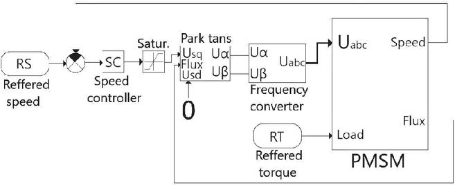
Figure 1 Structure of the model.
A control system of the AC motors (in this study case PMSM) utilizes a special coordinates for description of control laws. The main control signals are calculated in rotational coordinate system, and then transform to stationary system due to trigonometrical equations. The rotational speed of coordinates depends on speed of rotor.
The equilibrium state equations of stator are needed for the creation of stable control in stationary coordinate system.
| (1) |
where , , , , – stator’s voltages and currents in , axes, , – stator’s flux in , axes, – stator resistance [7].
The same equations in the dq coordinate system:
| (2) |
where , , , – stator’s voltages and currents in d, q axes, , – stator’s flux in axes, – electrical speed of a rotor [7].
The PMSM control system is built in dq coordinates. Speed control is carried out by controlling the motor torque. If the stator current is oriented along the q axis, then it is expressed through the moment using relation (3) [7].
| (3) |
where – vector of stator’s current, T – electromagnetic torque, – number of poles pares, – speed of magnetic field. , because .
The whole system of equations of PMSM:
| (4) |
where – stator resistance, , – stator’s inductance in axes.
| (5) | |
| (6) | |
| (7) | |
| (8) |
In this study, case of non-salient-pole machine is utilized, following assumptions are applied:
| (9) |
An output of the speed controller (it is represented in Figure 1) is a torque component of current in rotational coordinate system. The saturation block is placed after the speed regulation block. It is necessary, because of increasing electromagnetic torque and currents in the cases of fast transient process systems.
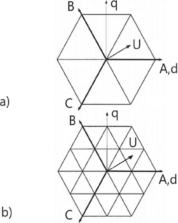
Figure 2 Forming of Vector PWM for: (a) two – level inverter, (b) three – level inverter.
The Reverse Park Transformation (RPT) block consists of RPT and two current controllers (Torque and flux components, q and d corresponding).
Next block is the frequency converter with PWM unit. Two voltages and creates the vector which is rotating in this coordinate system. The whole coordinate system can be divided into 6 zones for two-lever inverter as shown on the Figure 2(a) and 24 zones for three-lever inverter as shown on the Figure 2(b).
Each edge of any of the triangles inside the hexagon corresponds to a certain combination of inverter power keys [8]. Two – level inverter has 6 iGBT-transistors and 8 combinations, three – level inverter has 12 iGBT-transistors and 27 combination. The topologies of inverters are presented in Figure 3.
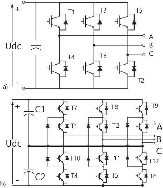
Figure 3 Topology of invertors: (a) two – level inverter, (b) three – level inverter.
The combination can be chosen by geometrical projection of vector on axes of three – phase coordinate system ABC or projection on triangle’s verge.This projection determines the time of combination’s work. The vector’s length of the determines the work of a zero vector.
The parameters of the modelled PMSM are represented below:
Table 1 Parameters of PMSM
| Parameters | Values |
| P, number of poles | 6 |
| R (stator resistance), Ohm | 1.4 |
| (stator flux), Wb | 0.1546 |
| Ld, H | 0.0066 |
| Rq, Ohm | 0.5 |
| Lq, H | 0.0066 |
| J (moment of inertia), kg* | 0.3 |
| B (friction coefficient) | 0.002 |
Observer inside the PMSM block is utilized to calculate the rotational speed of the motor. In the cases of system implementation, the filter is required due to noises and stochastic processes. Extended Kalman Filter (EKF) or Madgwick filter (MF) are well-known solutions [9]. The EKF filter was utilized in this study, as most common solution.
3 Comparison and Selection of Inverter
In this chapter, the comparison and selection of the most suitable invertor is described. The comparison of two-level and three level inverters is performed in the terms of the value of Total Harmonics Distortions (THD) of the output current on several frequencies of the current and amplitude of the current. A modulation coefficient M is changed also (the modulation coefficient determines the percentage of output voltage vector) [8]. The smaller THD is better due to decreasing of additional disturbances from electrical motor and thermal losses. The Fast Fourier Transform (FFT) in Matlab/Simulink was used for this analysis. The results of analysis are represented in Figures 4–6, and summarized in Table 2.
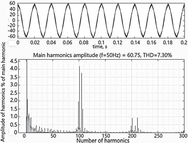
Figure 4 The spectral composition of the current at the output of the inverter at f 50 Hz and M 1 for two-level case.
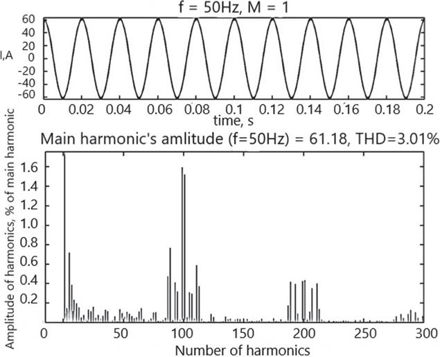
Figure 5 The spectral composition of the current at the output of the inverter at f 50 Hz and M 1 for three-level case.
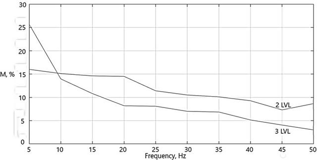
Figure 6 THD ratio on frequency.
Table 2 Values of THD on different modulation coefficients and frequencies
| Two-level Inverter | Three-level Inverter | ||||
| 50 | 1,15 | 8,65 | 50 | 1 | 3,01 |
| 45 | 1 | 7.30 | 45 | 0,95 | 4,05 |
| 40 | 0,9 | 9,27 | 40 | 0,86 | 5,14 |
| 35 | 0,75 | 10,1 | 35 | 0,73 | 6,85 |
| 30 | 0,64 | 10,5 | 30 | 0,62 | 7 |
| 25 | 0,57 | 11,4 | 25 | 0,52 | 8,09 |
| 20 | 0,33 | 14,5 | 20 | 0,43 | 8,19 |
| 15 | 0,3 | 14,6 | 15 | 0,31 | 10,8 |
| 10 | 0,27 | 15,1 | 10 | 0,21 | 13,95 |
| 5 | 0,21 | 16 | 5 | 0,1 | 25,67 |
According to the Figures 4–6 and Table 2, three-level inverter is better, because of lower THD values at the range of working frequencies of current (30–50 Hz). Three-level inverter produces current with higher amplitude and less exposure to high-order harmonics, which create additional heat losses. The data of Table 1 is represented in Figure 6 in graphical form.
According to the Figure 6, three-level inverter has higher amplitude of output current, and lower THD up to 10 Hz frequency. At the frequencies less than 10 Hz, the three-level inverter works worse, because of switching distortions, which depends on amount of power keys. Two-level inverter has better working characteristics at frequencies lower than 10 Hz, due to less number of iGBT transistors. For the work with lower frequencies a modification of PWM forming method is required, but such modification will destabilize the switching frequency. This task needs to be investigated.
4 Modelling with Different Load Modes
This chapter represents the modelling of the system with three types of the load: constant speed and variable load, variable speed and constant load, variable speed and variable load. In the cases of non-constant referred speed or torque, the forming is created in trapezoidal forms. An investigation of the system with step function as input of the system is needed before the main part of the modelling. The speed amplitude is 1000 rpm, torque is 40 Nm. The analysis of reaction is represented in Figure 7.
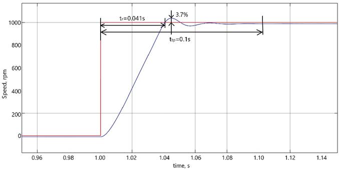
Figure 7 Speed reaction on step-function.
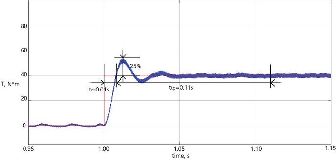
Figure 8 Torque reaction on step-function.
After the step function applied following results were obtained:
– Speed: response time – 0.041 s,
overshoot – 3.7%, transient process time – 0.1 s.
– Torque: response time – 0.01s, overshoot – 25%, transient process time – 0.11 s.
The torque overshoot is 25%, this value consider to be acceptable, however can effect rest of the system behavior. Also, overshoot can be decreased in a future with additional calibration of control system. The character of speed transient process is fluctuation damping, the torque’s one is complex (consists of several types of transient processes), because it looks like fluctuation damping process, but carry characteristic consists of small (amplitude around 1 N*m) fluctuations.
4.1 Constant Load, Variable Speed
The modelling of the work of the system with constant load (40 N*m) and variable speed (amplitude speed value 1000 rpm) is represented in Figures 9 and 10. This mode simulates lift applications.

Figure 9 Speed and torque graphics of “lift” mode.
The peak amplitude electromagnetic torque of the system is 70 Nm. The steady state amplitude electromagnetic torque of the system is 61 Nm. This difference can be explained in the terms of the inertia of the motor at the acceleration and deceleration moments. Equilibrium state of the system is reached for 0.04 s.
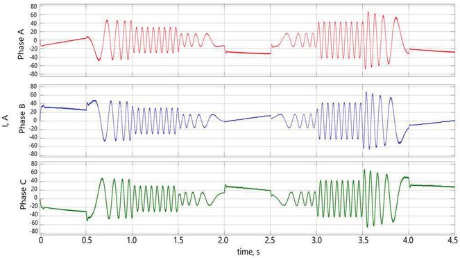
Figure 10 Currents graphics of “lift” mode.
According to Figure 10, three-phase output currents have the same form, but different phases and their summation is equal zero, that means the currents are formed correctly.
In the steady state mode, the average THD 7.54%. The influence of non-main harmonics less than 1%. The analysis of harmonics composition is necessary as harmonics of high order creates disturbances into magnetic field and it can increase the temperature of the electric motor and the system at general.
4.2 Constant Speed, Variable Load
The simulation of the work of the system with constant speed (1000 rpm) and variable torque (amplitude torque value 40 N*m) is represented in Figures 11 and 12. This mode can be correspond to the conveyer application.
In this case, the speed is increased up to nominal value for 0.3 s, as a motor cannot react on immediate change of the reference speed.
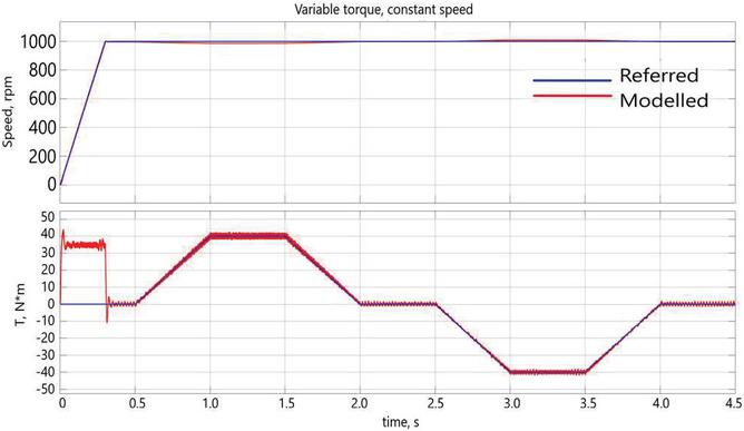
Figure 11 Speed and torque graphics of “mining” mode.
The electromagnetic torque (red characteristic) has the increasing during the start time, but after pre-acceleration, the moor works steady.
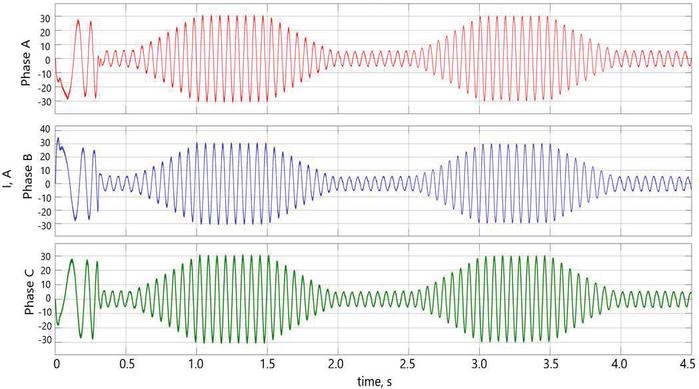
Figure 12 Currents graphics of “mining” mode.
In the steady-state mode, the average THD 6.31%. The influence of non-main harmonics less than 0.8%. The influence of variable torque on THD is higher, because of overshoot of transient processes of the torque.
4.3 Variable Load, Variable Speed
The simulation of the work of the system with variable speed (amplitude speed value 1000 rpm) and variable torque (amplitude torque value 40 N*m) is represented in Figures 13 and 14 below. This mode can represent steering applications. This mode combines previous two and requires higher accuracy at systems tuning.
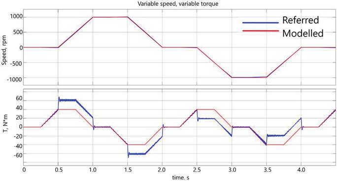
Figure 13 Speed and torque graphics of “steering” mode.
The electromagnetic torque differs in comparison with load torque, due to accelerations and decelerations of the electric motor. During the acceleration or deceleration, the system changes the electromagnetic torque of the motor to keep the constant state.
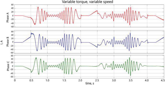
Figure 14 Currents graphics of “steering” mode.
In the steady-state mode, the average THD 9.19 %. The influence of non-main harmonics less than 1.5 %. The influence of combination of variable torque and variable speed on THD is higher, because of complex overshooting of transient processes of the torque and speed.
4.4 Comparison of Modes
During the modelling, the system demonstrated different behaviour. Also, the output currents were distorted in varying degrees, because of physical difference between speed and torque.
Table 3 Values of THD on different modulation coefficients and frequencies
| Application | THD, % | Influence of Harmonics, % |
| Lift-lowering | 7.54 | 1.0 |
| Conveyer | 6.31 | 0.8 |
| Steering | 9.19 | 1.5 |
A reducing of THD and its influence is possible by using Invertor with higher degree of levels and additional cross-linkages compensators in the control system.
The percentage of distortions and influence of undesirable factors increases with increasing of the systems difficulty.
Conveyers have the lowest THD, consequently constant-speed applications can be implemented easier, than others. The steering applications is the most difficult, because of combined transient processes.
5 Conclusion
After the investigation of the model next results were obtained for pump-controlled systems:
– Steering applications need higher power supply, because of cases of counter directions of load and acceleration;
– Mining applications must be launched without any additional load, because of stall currents;
– Invertors with higher voltage levels have higher accuracy and lower THD;
– Complexity of the whole system increases the THD and influence of higher order harmonics;
– Torques transient processes need more time for reaching the equilibrium state, consequently regulation of the speed easier;
– Lower THD decreases electromagnetic pulsations and torque ripples as result;
– The influence of frequency PWM can be fatal at the frequencies more than 5000 Hz and lower than 900 Hz, the best range is 1000 Hz–2000 Hz;
– Compensators in the control system can decrease the instability;
– Best working range of the motor is 25–50 Hz;
– Different frequencies have their own optimal modulation coefficient M, due to maximal output amplitude of the current.
– Hydraulic influence can add undesirable harmonics in the work cycles, consequently the impact of own motor’s needs to be minimized as possible.
References
[1] Noah D. Manring, Roger C. Fales, Hydraulic Control Systems, John Wiley & Sons 2019.
[2] Qingbo Guo, Cheng Ming Zhang, Liyi Li, Jiangpeng Zhang, Mingyi Wang, Maximum Efficiency Control of Permanent-Magnet Synchronous Machines for Electric Vehicles, The 8th International Conference on Applied Energy – ICAE2016.
[3] Christopher Goldenstein, Advanced Combustion Engines, Stanford University, 2011.
[4] Saša Milojević and Radivoje Pesic, CNG buses for clean and economical city transport, 2011.
[5] D. Grahame Holmes, Thomas A. Lipo. Pulse width modulation for power converters. Principles and practice. – Canada: A John Wiley & Sons, Inc., Publication, 2003.
[6] G.G. Sokolovskiy. AC drives with frequency regulation. Moscow Academa, 2006.
[7] A.B. Vinogradov. Vector control of alternating current electric drives. State educational institution of higher professional education “Ivanovo State Energy University”. – Ivanovo, 2008.
[8] D.G. Holmes, “A general analytical method for determining the theoretical harmonic components of carrier based PWM strategies”, Industry Applications Conference, Thirty-Third IAS Annual Meeting. The 1998 IEEE, Vol. 2, 12–15 Oct. 1998.
[9] Peter S. Maybeck, Stochastic Models, Estimation and Control, Academic Press, 1982.
[10] D. Casadei, F. Profumo, G. Serra, A. Tani, ”FOC and DTC: two viable schemes for induction motors torque control”, IEEE Transactions on Power Electronics, Vol. 17, Issue: 5, Sept. 2002.
Biography

Viacheslav Zakharov Doctoral student of Tampere university, Finland. Master of science in Control systems and Automation.
International Journal of Fluid Power, Vol. 24_1, 125–140.
doi: 10.13052/ijfp1439-9776.2416
© 2023 River Publishers