Predicting Hydraulic Oil Thermophysical Properties Using Physics-Informed Neural Networks
Ahmad Al-Issa* and Jürgen Weber
Chair of Fluid-Mechatronic Systems, TU Dresden, Dresden, Germany
E-mail: ahmad.alissa.85.85@gmail.com
*Corresponding Author
Received 13 November 2023; Accepted 22 April 2024
Abstract
The thermophysical properties of hydraulic oil, density, viscosity, thermal expansion, and compressibility, are pivotal factors influencing the functioning of hydraulic systems. With the multitude of hydraulic oils available for use, conducting numerous experiments to determine their specifications under different temperatures and pressures, or devising new empirical correlations, becomes a costly and time-consuming endeavour. Therefore, it becomes imperative to establish an efficient and comprehensive model based on minimal experimental data. This study adopts Physics Informed Neural Networks (PINNs) to design new correlation model to predict variations in hydraulic oil specifications using only 30 empirical data sets as a best-case scenario, enabling the prediction of 10,000 points spanning temperatures (20–100)C and pressures (0–300) bar. The results derived from the PINN model exhibit favourable high accuracy, reaching up to 99.96% when compared to empirical correlations results.
Keywords: Hydraulic oil, thermophysical properties, physics informed neural networks.
1 Introduction
The majority of currently used hydraulic oils are derived from mineral oil, chosen primarily for their cost-effective performance [1]. Hydraulic oil serves the crucial function of facilitating power transmission in hydraulic systems, ensuring the efficient operation and durability of components like pumps and actuators that experience relative movement at high speeds, pressures, and temperatures. When selecting mineral oil for a hydraulic system, it is essential to consider specific system requirements and operating conditions, including temperature, pressure, load, speed, and equipment type. The density and viscosity of hydraulic oil play a pivotal role in pump efficiency, contamination control, pressure loss, leakage prevention, lubrication, and addressing challenges like oil cavitation [2–5]. Additionally, hydraulic oil specifications, including isobaric thermal expansion and isothermal compressibility, are vital for maintaining overall system performance efficiency and temperature management.
Since decades, several empirical correlation equations have been developed by researchers for the purpose of determining thermophysical properties of hydraulic oils with temperature-pressure relationship. However, these correlations need for extensive laboratory experiments spanning the entire specific range of temperature and pressure. Therefore, these correlations fail to predict properties at wider range of operating conditions but work well in the limited circumstances and types where the data used to develop them came from.
Therefore, to avoid the costs of experiments and time, soft computing methods have been used to predict the thermophysical properties of mineral oil. Among these methods, we can point to the classical artificial neural network (ANN) as the most widely alternative methods. In this regard, numerous studies have been performed on specification of various fluids by employing neural networks. Some of the studies worth mentioning are summarized in Table 1. It can be classified the oils that have been studied into three groups. Lubricant oils, heavy oils, and crude oils.
For lubricant oils, Afrand et al. [6], Haldar et al. [7], and Loh et al. [8] proposed neural networks for the purpose of improving viscosity prediction of lubricating oils and compared them with experimental results or with empirical correlations. For example Afrand et al. propos an optimal artificial neural network (ANN) to predict the relative viscosity of MWCNTs-SiO2/AE40 nano-lubricant using experimental data. The ANN model is found to be more accurate compared to the empirical correlation, with a deviation margin of 1.5% compared to 4% in the correlation.
Regarding to heavy oil, Pan et al. [9], and Alade et al. [10] studied the feasibility of using neural networks to predict the viscosity of heavy oils. For instance, Pan et al. present a method based on the Process Neural Network (PNN) to predict the viscosity of heavy oil in high water cut stage. Their method takes into account input parameters such as temperature, water cut, and API to accurately measure the viscosity of heavy oil. They concluded that the reliability and accuracy of the PNN model for predicting oil viscosities is better compared to traditional methods, with small computation errors.
Concerning crude oils, Omole et al. [11], Torabi et al. [12], Makinde et al. [13], Lashkenari et al. [14], Ghorbani et al. [15], Hadavimoghaddam et al. [16], Gao et al. [17] implemented machine learning for crude oils. Hadavimoghaddam et al. implemented six machine learning models to predict dead oil viscosity with 2247 pressure-volume-temperature (PVT) data were used for developing and testing these models, covering a wide range of viscosity data from light intermediate to heavy oil and found that the Super Learner model outperformed other machine learning algorithms and common correlations based on metric analysis. It can potentially replace empirical models for viscosity predictions on a wide range of viscosities. While Gao et al. proposed a method for predicting the viscosity of heavy crude oil diluted with lighter oils using machine learning techniques. It collects 156 viscosity datasets from openly published literature and compares the performance and accuracy of the proposed model with existing empirical correlations and experimental values. The new viscosity model outperforms existing empirical correlations and shows higher accuracy in predicting the viscosity of diluted heavy crude oil.
The primary findings from all these research studies indicate that they are exclusively founded on data-driven methodologies which mean there is no physic help training their neural networks. Conversely, a review of the literature unveils the absence of any documented endeavours to model the thermophysical properties of hydraulic oils used within hydraulic systems, such as HLP and HM (ISO Grade 32, 46 and 68), using techniques like physics-informed neural networks or even traditional neural networks.
Therefore, the main purpose of this study is to fill this research gap and design a new correlation model based on Physics Informed Neural Networks employing a few amounts of empirical data to estimate thermophysical properties of hydraulic oils, making it easily applicable in hydraulic oils fields.
Table 1 The summary of the fluids data set and its ranges of temperature and pressure used in neural networks
| Authors | Fluid | Data Set | TemperatureC | Pressure Bar |
| Omole et al. (2009) | Crude Oil | 32 | 67.7 – 112.2 | 98 – 334 |
| Torabi et al. (2011) | Crude Oil | 5 groups | 52.2 – 131.11 | 220 – 367.5 |
| Makinde et al. (2012) | Crude Oil | 105 | 52 – 142.7 | 25.8 – 429 |
| Lashkenari et al. (2013) | Crude Oil | 720 | – | – |
| Afrand et al. (2016) | lubricants | 48 | 25 – 60 | – |
| Ghorbani et al. (2016) | Crude Oil | Over 600 | 37.77 – 121.11 | 110 – 4790 |
| Pan et al. (2018) | heavy oil | 17 | 19 – 77 | – |
| Alade et al. (2019) | heavy oil | 2 groups | 70 – 150 | 0 – 70 |
| Loh et al. (2020) | lubricants | 3 groups | 10 – 100 | 0 |
| Haldar et al. (2020) | lubricants | 2 groups | 10 – 80 | – |
| Hadavimoghaddam et al. (2021) | Crude Oil | 2247 | 40 – 233.6 | – |
| Gao et al. (2022) | Crude Oil | 156 | 20 – 60 | – |
2 Hydraulic Oil Density and Viscosity as a Function of Temperature and Pressure
2.1 Oil Density
Witt has proposed a complex and nonlinear relationship that accurately relates the density of the oil to both pressure and temperature. This relationship provides a reliable method for determining the density of hydraulic oil under varying pressure and temperature conditions [18–20]. If density curve is concave or straight, the relationship is Equation (1) or, if the curve is convex or straight, the relationship is Equation (2.1):
| (1) | ||
| (2) |
Nevertheless, for a sufficiently restricted range of pressure, the densities of most liquids vary more with temperature than with pressure such that pressure can be omitted from the analysis [21]. For this reason, the density of liquids often is assumed to be constant with respect to pressure. A good approximation for the temperature dependence of the density at ambient pressure or restricted range of pressure, is the linear expression, Equation (3), [22].
| (3) |
Furthermore, despite being an approximation, Equation (4) can be derived as a straightforward formula for density concerning temperature and pressure when assuming isobaric coefficients of thermal expansion and thermal compression as constants of 7 10-4 1/K and 6.0606 10 1/pa respectively [23]. This derivation is based on fundamental principles of thermodynamics [21].
| (4) |
Table 2 Viscosity-temperature equations [24–27]
| Author or Standard | Equation |
| ASTM-D341-03 | |
| Reynolds | |
| Slotte | |
| Vogel | |
| Walther |
2.2 Oil Viscosity
The dynamic viscosity of an oil undergoes substantial changes in response to temperature variations. Typically, as temperature rises, the viscosity of an oil decreases. This is attributed to the increased thermal agitation of oil particles, allowing them to move more easily past one another. However, the rate of viscosity decrease can vary based on the unique properties of the oil. Researchers have developed various equations to estimate the temperature dependence of viscosity. These equations encompass both empirical relationships derived from experimental data and theoretical models. Table 2 presents the most frequently employed equations for calculating viscosity temperature dependence.
The impact of pressure on viscosity is a more intricate phenomenon and can vary based on the specific characteristics of the oil. Generally, as pressure increases, the viscosity of an oil tends to increase as well. This can be attributed to the compression of oil molecules under higher pressures. However, this effect is typically more significant at elevated pressures and may be influenced by the compressibility of the oil. To model the combined influence of temperature and pressure on viscosity, various equations of state are utilized. These equations provide a framework for describing the thermodynamic properties of oils. In Table 3, you can find some of the commonly employed equations of state that account for the simultaneous effects of temperature and pressure on viscosity.
Table 3 Viscosity-pressure equations [28–30]
| Author or Standard | Equation |
| API | |
| Barus | |
| Roelands |
2.3 Proposed Empirical Equation for Viscosity
Proposing to combine Vogel’s equation with the API equation, a comprehensive equation can be formulated, Equation (5). This equation is able to calculate viscosity considering both temperature and pressure variations.
| (5) |
As clear, this formula includes three correlation parameters a, b, and c which are determining for each kind of oil. In Appendix A, a mathematical producer is explained how to calculating these parameters.
Having comprehensive empirical correlations, Equations (4) and (5), it can be now accurately quantifying changes in both density and dynamic viscosity as functions of temperature and pressure.
3 Training Data Generation
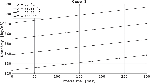
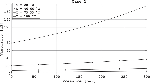
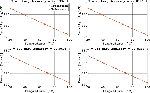
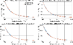
Using empirical correlations, a limited data set have been generated for the purpose of developing and training the neural network that covers some points in the range of temperature (20–100)C and pressure (0–300) bar. The pressure range is divided into only 6 distinct values. For each pressure value, 4 and 5 corresponding temperature values is selected. Consequently, the total number of empirical data set used of calculated density and viscosity amounted to 24 values for Case 1, and 30 values for Case 2. Although it is possible to generate a significantly larger training dataset, it is intentionally limited it to a maximum of 30 data points. This decision allows us to gauge the neural network’s performance and assess its ability to learn effectively. Figures 1 and 2 show the empirical data sets of case 1 for density and viscosity of the hydraulic oil HLP 32 respectively.
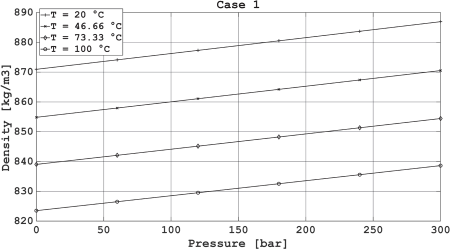
Figure 1 The calculated density for training purposes, Case 1.
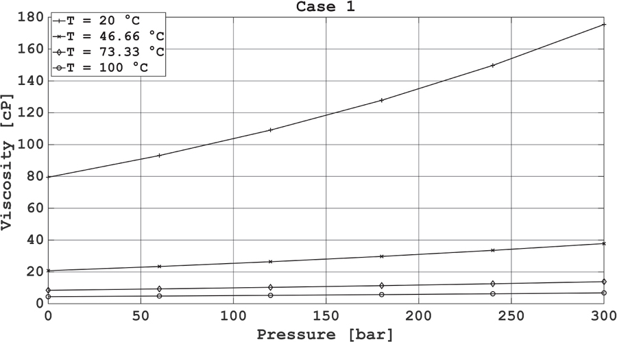
Figure 2 The calculated viscosity for training purposes, Case 1.
4 Physics-Informed Neural Networks
The traditional neural networks are based entirely on a data-driven approach that does not take into account the physical laws that are contained in the data. In contrast, physics-informed neural networks [31–33] introduce a machine learning framework that offer an approximate solution to PDEs by incorporating physical laws or constraints as additional loss terms during the training process. By doing so, PINNs can leverage both the available data and the underlying physics to provide accurate and robust solutions.
However, PINNs also come with some challenges. They require a significant amount of data for training, which can be expensive or difficult to obtain for certain physical systems. The choice of loss function and the architecture of the neural network can also greatly influence the accuracy and convergence of the solution. Additionally, the training process may require careful tuning of hyper parameters and regularization techniques to prevent overfitting or under fitting.
4.1 Governing Physical Equations
It is important to note that the specific implementation of PINNs will depend on the governing physics equations at hand and the data available. The effectiveness of loss function, network architecture, and training strategy will vary based on these equations being solved and the specific requirements of them.
Depending on the thermodynamic basics, it can be derived a particularly useful empirical equation of state that can be used to approximate the behavior of many hydraulic oils. For the density of oil, it can be considered as a function of pressure and temperature, Equation (6). Therefore, the overall change in density can equal the summation of change in density at constant temperature and pressure respectively, Equation (7) [21]
| (6) | |
| (7) |
As terms in temperature and pressure are distinct, it is assuming that thermal and pressure effects are decoupled. Thus, a change in temperature, for example, does not lead to a significant change in pressure. The small changes and associated with small changes in temperature and pressure can be approximated using a Taylor expansion to get Equation (8) without showing the necessary steps [21].
| (8) |
On the same foundation, both temperature and pressure varying can influence the viscosity of an oil, Equation (9). Changes in temperature and pressure can affect the oil’s molecular structure, intermolecular forces, and flow behavior, which can result in changes in its viscosity.
| (9) |
Skripov and Faizullin [34, 35] conducted an extensive study comparing liquid-vapor and liquid-solid phase transitions, wherein they examined the relationship between viscosity and temperature as well as pressure across various categories of liquids.
They focused their analysis on scenarios where the liquid’s thermal expansion coefficient is positive. Combining literature findings with their own results, those authors concluded that the following relations must be satisfied and [36]. These relations suggest that viscosity should decrease with rising temperature under isobaric processes, and conversely, increase with increasing pressure under isothermal conditions. Furthermore, by regarding viscosity as a function of pressure and temperature according to Equation (9), they formulated the subsequent identity:
| (10) |
Considering the viscosity dependencies outlined by and , they deduced that the inequality must be satisfied. To maintain viscosity constant, it is necessary to ensure that the total volume of the system remains unchanged when both pressure and temperature are varied slightly by and , respectively. Then, from Equation (8), the following result is obtained:
| (11) |
With Equation (10), we finally obtain
| (12) |
Simultaneously, it can be extracted additional properties of hydraulic oil; thermal expansion (), and compressibility () from Equations (8) and (12) during implementation of the current PINN model as explained in the following:
| (13) | ||
| (14) |
Basically, these equations are the gateway to understanding how easily oil can be compressed and how it responds when it either contracts or expands due to temperature and pressure changes.
4.2 Loss Function
In physics-informed models, the loss function is defined as the mean squared residuals of the data along with the mean squared errors of the associated governing PDEs [37] as it is illustrated in Equations (15), (16), (17), (18), and (19). It is designed to minimize the discrepancy between the predictions output of the neural network and the reference data, by satisfying the constraints imposed by the PDEs [31–33].
| (15) | ||
| (16) | ||
| (17) | ||
| (18) | ||
| (19) |
and are the loss-function components corresponding to the data and the governing partial equations, respectively. Here, represents the number of points for which the residual of the PDEs equations is calculated (the so-called collocation points) and is the number of training samples on the domain [38]. The reference or training data could be the exact analytical solutions of PDEs if applicable, solutions obtained using high-fidelity numerical solvers, or reliable experiments in labs.
4.3 PINN Model Structure and Implementation
This section aims to emphasize the effectiveness of the PINN model of this study in solving partial differential equations pertaining to hydraulic oil properties. In order to illustrate this methodology, mineral hydraulic oil with the classification type HLP 32 is utilized as a case study, while noting that the same approach can be applied to other types of hydraulic oils.
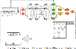
The algorithm displayed in Figure3 explained the customized design for predicting density and viscosity, solely relying on two input parameters: temperature and pressure. A typical architecture of Physics-Informed Neural Networks consists of six essential elements: input layer, hidden layer, output layer, secondary output, automatic differentiation, and loss function. These components within the neural network are responsible for approximating the solution to the partial differential equations, enabling the accurate prediction of density and viscosity values.
By leveraging this architecture, the proposed algorithm demonstrates the ability to accurately diagnose complex behaviors of hydraulic oil specifications for the complete temperature and pressure fields even with limited experimental observations are available. The developed PINN model was employed to predict 10,000 data points that span the same specific pressure and temperature range of generated empirical data set. We selected 250 pressure points and 40 corresponding temperature points for each pressure value to ensure that the network’s outputs adhere to Equations (8) and (12).
In this study, two activation functions are used for investigating their performance during the training, Tanh and Sigmoid [39]. The Tanh activation function and its derivative can be expressed as follows:
| (20) | ||
| (21) |
While the sigmoid activation function and its derivative are computed as:
| (22) | |
| (23) |
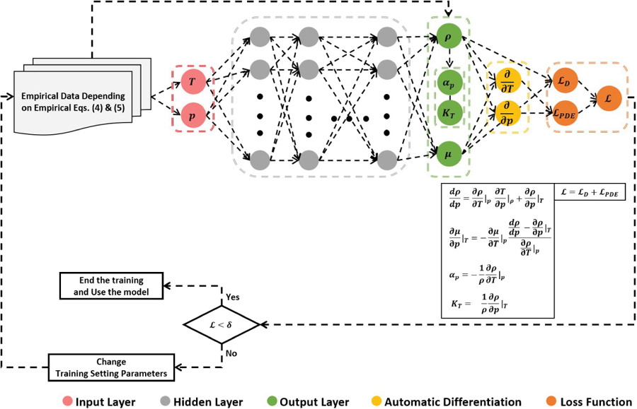
Figure 3 The schematic diagram of the current PINN model.
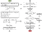
Knowing the ideal configuration of a deep neural network, which encompasses parameters like number of layers, number of neurons per layer, weight decay, and learning rates, is a challenging endeavor, often requiring exploration through trial and error. For instance, weight decay, used for regularization in neural networks, may be initially set at a low value (e.g., 0.001) and iteratively increased until network performance begins to deteriorate. The value at which performance degradation initiates signifies the optimal weight decay value for the network.
Therefore, a fully connected neural network starting with 1 hidden layer and 300 neurons per layer as initial number is employed. A mini batch size for network training of 50 samples is used for both data and residual points. To train the network, only 1000 epochs with learning rates of 0.01 is used.
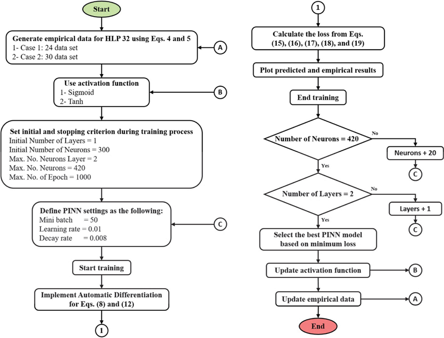
Figure 4 Proposed algorithm to find the optimal PINN model.
Generally, the ADAM optimizer [40], an adaptive algorithm for gradient-based first-order optimization is used to optimize the model parameters (Weights and Basis). Automatic differentiation (AD) [31, 41, 42] is applied to differentiate outputs with respect to the inputs to construct density and viscosity Equations (8) and (12). The PINN model uses automatic differentiation to represent all the differential operators and hence there is no explicit need for a mesh generation.
The proposed algorithm to find the optimal neural network is illustrated in Figure 4. Table 4 shows the related optimum training settings parameters of the existing PINN model on which the neural network is run based on them. These optimal settings have been reached after hundreds attempts.
Table 4 Optimum parameters for the PINN model
| Setting Parameter | Value |
| No of hidden layer | 2 |
| No of neurons per layer | 400 or 420 |
| No of epoch | 1000 |
| Learning rate | 0.01 |
| Decay rate | 0.008 |
| Empirical training data | 30 |
| Predicted data | 10,000 |
| Mini batch | 50 |
| Activation Function | Sigmoid |
| Optimizer | ADAM |
5 Results and Discussion
For each of two cases of data set, Sigmoid and Tanh activation function are used. Tables 5 and 6 illustrates the impact of the number of neurons on the loss, training time and simulation time for all number of neurons used for each case.
In Case 1, employing the Sigmoid function, the minimum loss was registered at 2.45E-06, while for Case 2, it stood at 2.53E-06 with 400 neurons utilized in both scenarios. Conversely, for Case 1, utilizing the Tanh function, the minimum loss was noted as 1.00E-05, while for Case 2, it amounted to 1.62E-05 with 320 neurons employed in both cases. Despite the lower minimum loss recorded in Case 1 when using the Sigmoid function, the accuracy remains inferior compared to Case 2, attributed to insufficient data availability.
Therefore, it can be seen that the value of the loss function of Case 2 using Sigmoid function with (400 or 420) neurons reached a smaller value in the end and represented the best scenario in terms of data quantity, time-consuming and the achieved accuracy. The lower loss values indicate these number of neurons can better fit the training pressure traces.
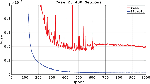
Figures 5 and 6 show the convergences history of the total training loss function of the PINN model for Sigmoid and Tanh respectively. Through investigating the activation functions performance and comparing their results, it was found that the best activation function is the sigmoid function in the case of the presence of 420 neurons or less. While when using the Tanh function, the stochastic gradient descent in the losses caused clear oscillations, which allows a better Sigmoid function generalization for the current PINN model.
Table 5 Total, data, and PDEs loss for the last training epoch with the elapsed time for different sizes of PINN model and for two data sets using Sigmoid function
| Loss | Training | Simulation | |||
| No Neurons | Total | Data | PDEs | mm:ss | ss.sss |
| Case 1: Data 24 | |||||
| 300 | 2.75E-06 | 2.03E-07 | 2.54E-06 | 40:27 | 01.265 |
| 320 | 2.68E-06 | 2.09E-07 | 2.47E-06 | 44:35 | 00.235 |
| 340 | 2.97E-06 | 2.17E-07 | 2.75E-06 | 52:55 | 00.443 |
| 360 | 2.89E-05 | 1.69E-06 | 2.72E-05 | 47:34 | 00.336 |
| 380 | 2.56E-06 | 1.52E-07 | 2.41E-06 | 51:57 | 00.488 |
| 400 | 2.45E-06 | 2.70E-07 | 2.18E-06 | 48:12 | 00.272 |
| 420 | 3.36E-06 | 1.24E-07 | 3.24E-06 | 51:51 | 00.221 |
| Case 2: Data 30 | |||||
| 300 | 3.13E-06 | 4.17E-07 | 2.71E-06 | 38:41 | 01.503 |
| 320 | 3.03E-06 | 2.24E-07 | 2.80E-06 | 45:49 | 00.522 |
| 340 | 3.21E-06 | 3.21E-07 | 2.89E-06 | 53:54 | 00.487 |
| 360 | 1.73E-05 | 1.23E-07 | 1.71E-05 | 51:28 | 00.462 |
| 380 | 4.70E-06 | 1.62E-07 | 4.54E-06 | 52:27 | 00.360 |
| 400 | 2.53E-06 | 1.92E-07 | 2.34E-06 | 49:51 | 00.438 |
| 420 | 2.55E-06 | 1.35E-07 | 2.41E-06 | 35:26 | 01.131 |
Table 6 Total, data, and PDEs loss for the last training epoch with the elapsed time for different sizes of PINN model and for two data sets using Tanh function
| Loss | Training | Simulation | |||
| No Neurons | Total | Data | PDEs | mm:ss | ss.sss |
| Case 1: Data 24 | |||||
| 300 | 3.02E-05 | 1.38E-05 | 1.64E-05 | 49:39 | 00.433 |
| 320 | 1.00E-05 | 2.58E-06 | 7.46E-06 | 46:10 | 01.452 |
| 340 | 2.02E-05 | 5.02E-06 | 1.52E-05 | 46:01 | 00.514 |
| 360 | 1.48E-05 | 3.85E-06 | 1.09E-05 | 51:59 | 00.291 |
| 380 | 1.54E-05 | 5.68E-06 | 9.68E-06 | 49:00 | 00.445 |
| 400 | 1.03E-05 | 4.54E-06 | 5.80E-06 | 53:20 | 00.231 |
| 420 | 1.03E-05 | 5.91E-06 | 4.39E-06 | 53:25 | 00.490 |
| Case 2: Data 30 | |||||
| 300 | 1.69E-05 | 3.86E-06 | 1.30E-05 | 35:09 | 00.557 |
| 320 | 1.62E-05 | 1.09E-05 | 5.26E-06 | 45:25 | 00.309 |
| 340 | 5.29E-05 | 5.99E-06 | 4.69E-05 | 35:53 | 00.401 |
| 360 | 9.08E-05 | 2.11E-05 | 6.97E-05 | 47:57 | 00.404 |
| 380 | 2.67E-05 | 1.57E-05 | 1.10E-05 | 49:00 | 00.448 |
| 400 | 3.90E-05 | 9.48E-06 | 2.95E-05 | 42:32 | 00.739 |
| 420 | 4.16E-05 | 1.30E-05 | 2.86E-05 | 44:00 | 00.231 |
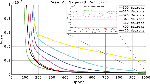
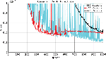
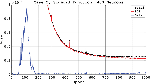
We present the history of different losses over the total 1000 epochs in Figure 7. Although the PDEs residual has the largest loss, each term has a value lower than 3E-06, indicating a convergence at the final epoch. Figure 8 shows the difference of the total training losses using the two activation functions Sigmoid and Tanh. Where the differences are clear in the minimum value that was reached and smoothness of convergences history.
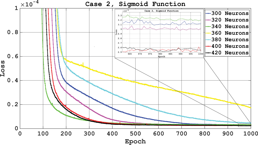
Figure 5 Total training loss vs. number of epochs.
Following the completion of training, the predicted results of density and viscosity are evaluated by comparison with empirical findings from Equations (4) and (5) during the normalization of errors and accuracy function which are computed as:
| (24) | ||
| (25) |
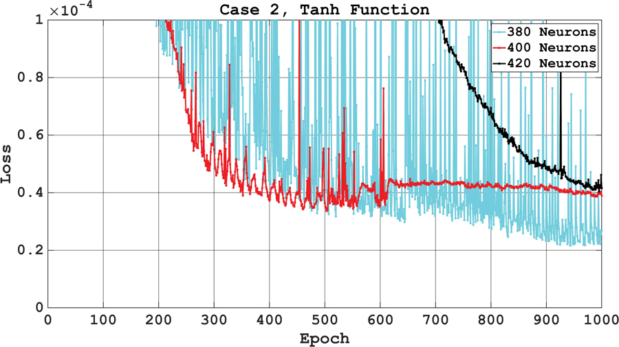
Figure 6 Total training loss vs. number of epochs.
Figure 7 Loss during the training process using Sigmoid function.
Figures 9 and 10 are displayed randomly chosen examples of plotting corresponding density and viscosity curves at each temperature point for pressure values of (0, 90, 190, and 255) bar for density and viscosity. However, Figures 11 and 12 depict the entire spectrum of density and viscosity alterations under the influence of pressure and temperature. Notably, the maximum error observed in the density evaluations was found to be only 0.37%, while it was 4.42% in the viscosity evaluations, indicating a high satisfactory level of precision in the neural network’s predictions. The accuracy is computed over the entire investigated domain.
In Table 7, it has been presented the results obtained from the Equations (13) and (14) for calculating the thermal expansion and compressibility of hydraulic oil HLP 32 for over a wide range of pressures (0–300) bar. These values are the average value for a range of temperatures (20–100)C. By observing these values, we can find the extent to which they correspond to the practically measured data for thermal expansion 7 10 1/K and compressibility 6.0606 10 1/pa.
Figure 8 Total loss during the training process verses activation functions.
Figure 9 Simulation results and the absolute accuracy for the density using PINN model in comparison with the reference data.
Figure 10 Simulation results and the absolute accuracy for the viscosity using PINN model in comparison with the reference data.
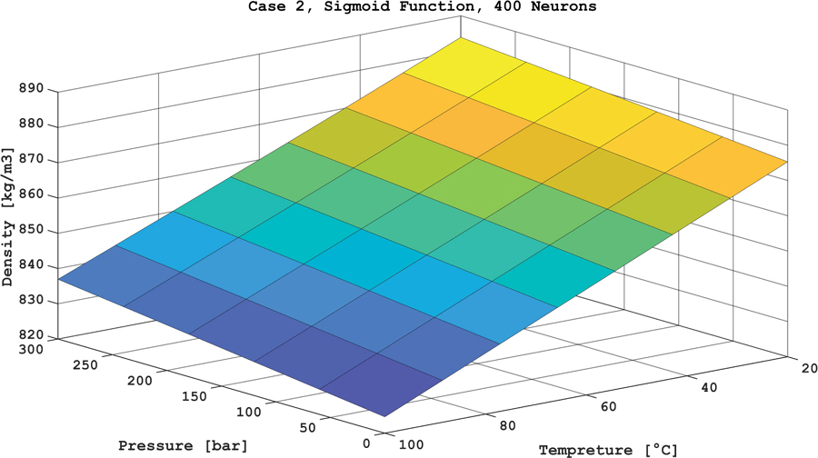
Figure 11 Density of hydraulic oil HLP 32 as a function of T and p using PINN model.
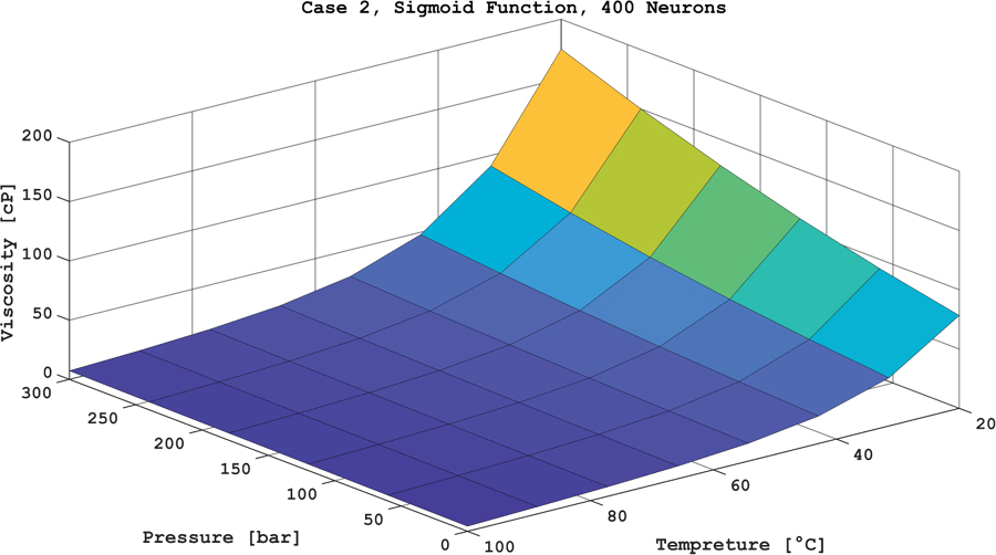
Figure 12 Viscosity of hydraulic oil HLP 32 as a function of T and p using PINN model.
Table 7 Thermal expansion and compressibility of hydraulic oil HLP 32
| Pressure (bar) | Thermal Expansion 10 (1/K) | Compressibility 10 (1/pa) |
| 0 | 6.982 | 0.47 |
| 50 | 6.948 | 5.26 |
| 100 | 7.017 | 6.11 |
| 150 | 6.862 | 5.16 |
| 200 | 7.026 | 6.12 |
| 250 | 6.913 | 5.92 |
| 300 | 7.046 | 6.09 |
PINN model of this study was coded using MATLAB language and the training process was conducted on a PC equipped with an Intel Core i5 processor and 32 GB of RAM.
6 Conclusion
This study presents a promising PINN model to predicting 10,000 points of the thermophysical properties of hydraulic oil HLP 32 for range of temperature (20–100)C and pressure of (0–300) bar utilizing only 30 empirical data sets. Employing the proposed PINN model, it becomes feasible to depend on limited amount of empirical or experimental data, eliminating the necessity to carry out numerous laboratory experiments across all temperatures and pressures range.
Validity and accuracy of this model has been established by comparing the obtained results of this model and the existing correlations for hydraulic oils. It is founded that the best predictive properties in terms of the ratio of accuracy and computational costs have a neural network with 2 hidden layers, (400 or 420) neurons, trained employing the ADAM optimizer and using Sigmoid activation function. For it, the average relative deviation of the predicted and reference density values was 0.37%. For viscosity, this indicator was 4.42%.
All this makes it possible to talk about the prospects of PINN models for predicting the thermophysical properties of hydraulic oils in the practical work of companies dealing with the production of hydraulic oils.
Future endeavours for researchers interested in this field of neural networks could entail exploring the additional oil properties such as enthalpy, isobaric specific heat capacity, thermal conductivity, and so on.
Authors’ Contributions
A.A.: Analysis, Conceptualization, Methodology, Neural Network Coding, Writing, Editing. J.W.: Supervision, Reviewing, Project Administration. All authors have read and agreed to the published version of the manuscript.
Data Availability Statement
Not applicable.
Conflicts of Interest
The authors declare no conflict of interest.
Appendix A: Proposed Mathematical Procedures to Determine Empirical Parameters
This study focuses on the prevalent hydraulic oil types, HM and HLP, to develop a mathematical model for analysis. We will elucidate the mathematical procedures utilized to calculate viscosity based on temperature and pressure. The model aims to provide a comprehensive understanding of how viscosity varies with changes in temperature and pressure. We will employ the commonly used equations Vogel and API in our approach, which consists of the following steps:
We will acquire experimental data through measurements reported in the literature [43–46] for the two categories of hydraulic oil (HM, and HLP) with ISO VG 32, ISO VG 46, and ISO VG 68 grades. For each oil type, we will obtain a single density value at 15C, along with kinematic viscosity values at three distinct temperatures as depicted in Table A.1.
Utilizing Equation (3) and the experimental results of density from literatures at 15 C as shown in Table A.1, we can calculate the density of the oil at atmospheric pressure and at specific temperatures, Table A.2.
By utilizing the known values of kinematic viscosity and density at specific temperatures from Tables A.1 and A.2, we can determine the dynamic viscosity using Equation (A.1), as shown in Table A.3.
| (A.1) |
By simultaneously forming and solving three equations using the Vogel Equation (A.2), we can calculate the constants a, b, and c for the tested hydraulic oils. The calculated values of these constants are presented in Table A.4. The time required for calculations is 39 seconds.
| (A.2) |
Table A.1: Kinematic Viscosity and density of testing hydraulic oils, at atmospheric pressure [43–46]
| ISO Grade 32 | ISO Grade 46 | ISO Grade 68 | |
| Hydraulic Oil HM | |||
| Density @ 15 (kg/m) | 871 | 876 | 882 |
| Kin. Viscosity, @ 20.5 C (mm/s) | 80.13 | 146.92 | 217.37 |
| Kin. Viscosity, @ 40 C (mm/s) | 30.32 | 48.5 | 68.3 |
| Kin. Viscosity, @ 100 C (mm/s) | 5.24 | 6.89 | 10.8 |
| Hydraulic Oil HLP | |||
| Density @ 15 (kg/m) | 874 | 879 | 884 |
| Kin. Viscosity, @ 0 C (mm/s) | 420 | 780 | 1400 |
| Kin. Viscosity, @ 40 C (mm/s) | 32.1 | 46.7 | 69.2 |
| Kin. Viscosity, @ 100 C (mm/s) | 5.4 | 6.9 | 8.9 |
Table A.2: Calculated density of testing hydraulic oils
| ISO Grade 32 | ISO Grade 46 | ISO Grade 68 | |
| Hydraulic Oil HM | |||
| Density @ 20.5 C (kg/m) | 867.65 | 872.63 | 878.61 |
| Density @ 40 C (kg/m) | 855.89 | 860.80 | 866.69 |
| Density @ 100 C (kg/m) | 820.68 | 825.39 | 831.05 |
| Hydraulic Oil HLP | |||
| Density @ 0 C (kg/m) | 883.22 | 888.27 | 893.33 |
| Density @ 40 C (kg/m) | 858.83 | 863.75 | 868.66 |
| Density @ 100 C (kg/m) | 823.51 | 828.22 | 832.93 |
Table A.3: Calculated dynamic viscosity of testing hydraulic oils
| ISO Grade 32 | ISO Grade 46 | ISO Grade 68 | |
| Hydraulic Oil HM | |||
| Dyn. Viscosity, @ 20.5 C (Pa.s) | 0.0695 | 0.1282 | 0.1909 |
| Dyn. Viscosity, @ 40 C (Pa.s) | 0.0259 | 0.0417 | 0.0591 |
| Dyn. Viscosity, @ 100 C (Pa.s) | 0.0043 | 0.0056 | 0.0089 |
| Hydraulic Oil HLP | |||
| Dyn. Viscosity, @ 0 C (Pa.s) | 0.3709 | 0.6928 | 1.2506 |
| Dyn. Viscosity, @ 40 C (Pa.s) | 0.0275 | 0.0403 | 0.0601 |
| Dyn. Viscosity, @ 100 C (Pa.s) | 0.0044 | 0.0057 | 0.0074 |
Table A.4: Calculated constants from Vogel equation for testing hydraulic oils
| Constants | ISO Grade 32 | ISO Grade 46 | ISO Grade 68 |
| Hydraulic Oil HM | |||
| a, (N/m)/sec | 7.483710 | 8.050910 | 3.124410 |
| b, K | 790.8969 | 801.0341 | 560.0949 |
| c, K | 177.9226 | 185.0062 | 206.3470 |
| Hydraulic Oil HLP | |||
| a, (N/m)/sec | 9.088610 | 9.888010 | 9.442410 |
| b, K | 731.1608 | 748.7341 | 807.5559 |
| c, K | 185.2091 | 188.5919 | -188.0670 |
Appendix B: Nomenclature
| Symbol | Description | Unit |
| Accuracy | – | |
| Constants for Witt equation | – | |
| Constants for Barus equation | – | |
| a, b, c, d | Constants for Slotte, Vogel, and Walther equations | – |
| Normalized error | – | |
| Compressibility | 1/pa | |
| Total loss function | – | |
| Loss function of data | – | |
| Loss function of data for density | ||
| Loss function of data for viscosity | ||
| Loss function of PDE | – | |
| Loss function of PDE for density | ||
| Loss function of PDE for viscosity | ||
| No. of training samples of data | – | |
| No. of training points of PDE | – | |
| Pressure | Bar | |
| Atmosphere pressure | Bar | |
| Reference pressure | Bar | |
| Temperature | C | |
| Absolute temperature | K | |
| Reference temperature at | C | |
| Reference temperature | C | |
| Kinematic viscosity at | mm/s | |
| Pressure-viscosity coefficient | – | |
| Density | ||
| Density at | ||
| Isobaric density | ||
| Reference density | ||
| Dynamic viscosity | ||
| Dynamic viscosity at | ||
| Change of temperature | C | |
| Change of pressure | Bar | |
| Change of density | ||
| Change of density at constant T | ||
| Change of density at constant p | ||
| Change of dynamic viscosity | cP | |
| Change of dynamic viscosity at constant T | cP | |
| Change of dynamic viscosity at constant p | cP | |
| pressure-viscosity coefficient | 1/bar | |
| Thermal expansion coefficient | 1/K |
References
[1] Totten, G.E.; Negri, V.J.D. Handbook of Hydraulic Fluid Technology; CRC Press, 2011; ISBN 978-1-4200-8527-3.
[2] Bair, S.; Michael, P. Modelling the Pressure and Temperature Dependence of Viscosity and Volume for Hydraulic Fluids. International Journal of Fluid Power 2010, 11, 37–42, doi:10.1080/14399776.2010.107 81005.
[3] Hodges, P. Hydraulic Fluids; Butterworth-Heinemann, 1996; ISBN 978-0-08-052389-7.
[4] Osterland, S.; Müller, L.; Weber, J. Influence of Air Dissolved in Hydraulic Oil on Cavitation Erosion. International Journal of Fluid Power 2021, doi:10.13052/ijfp1439-9776.2234.
[5] Zhang, J.; Qi, N.; Jiang, J. Effect of Oil Viscosity on Hydraulic Cavitation Luminescence. Fluid Dyn 2021, 56, 371–382, doi:10.1134/S00154 62821030125.
[6] Afrand, M.; Nazari Najafabadi, K.; Sina, N.; Safaei, M.R.; Kherbeet, A.Sh.; Wongwises, S.; Dahari, M. Prediction of Dynamic Viscosity of a Hybrid Nano-Lubricant by an Optimal Artificial Neural Network. International Communications in Heat and Mass Transfer 2016, 76, 209–214, doi:10.1016/j.icheatmasstransfer.2016.05.023.
[7] Haldar, A.; Chatterjee, S.; Kotia, A.; Kumar, N.; Ghosh, S.K. Analysis of Rheological Properties of MWCNT/SiO2 Hydraulic Oil Nanolubricants Using Regression and Artificial Neural Network. International Communications in Heat and Mass Transfer 2020, 116, 104723, doi:10.1016/j.icheatmasstransfer.2020.104723.
[8] Loh, G.C.; Lee, H.-C.; Tee, X.Y.; Chow, P.S.; Zheng, J.W. Viscosity Prediction of Lubricants by a General Feed-Forward Neural Network. J. Chem. Inf. Model. 2020, 60, 1224–1234, doi:10.1021/acs.jcim.9b01068.
[9] Pan, B.; Zhu, Y.; Wang, C.; Su, S. A Process Neural Network Model for Calculation of Heavy Oil Viscosity in High Water Cut Stage. Petroleum Science and Technology 2018, 36, 313–318, doi:10.1080/10916466.2017.1421973.
[10] Alade, O.; Al Shehri, D.; Mahmoud, M.; Sasaki, K. Viscosity–Temperature–Pressure Relationship of Extra-Heavy Oil (Bitumen): Empirical Modelling versus Artificial Neural Network (ANN). Energies 2019, 12, 2390, doi:10.3390/en12122390.
[11] Omole, O.; Falode, O.A.; Deng, A.D. Prediction of Nigerian Crude Oil Viscosity Using Artificial Neural Network. Petroleum & Coal 2009, 51, 181–188.
[12] Torabi, F.; Abedini, A.; Abedini, R. The Development of an Artificial Neural Network Model for Prediction of Crude Oil Viscosities. Petroleum Science and Technology 2011, 29, 804–816, doi:10.1080/10916460903485876.
[13] Makinde, F.A.; Ako, C.T.; Orodu, O.D.; Asuquo, I.U. Prediction of Crude Oil Viscosity Using Feed-Forward Back-Propagation Neural Network (FFBPNN). Petroleum & Coal 2012, 54.
[14] Lashkenari, M.S.; Taghizadeh, M.; Mehdizadeh, B. Viscosity Prediction in Selected Iranian Light Oil Reservoirs: Artificial Neural Network versus Empirical Correlations. Pet. Sci. 2013, 10, 126–133, doi:10.1007/s12182-013-0259-4.
[15] Ghorbani, B.; Hamedi, M.; Shirmohammadi, R.; Mehrpooya, M.; Hamedi, M.-H. A Novel Multi-Hybrid Model for Estimating Optimal Viscosity Correlations of Iranian Crude Oil. Journal of Petroleum Science and Engineering 2016, 142, 68–76, doi:10.1016/j.petrol.2016.01.041.
[16] Hadavimoghaddam, F.; Ostadhassan, M.; Heidaryan, E.; Sadri, M.A.; Chapanova, I.; Popov, E.; Cheremisin, A.; Rafieepour, S. Prediction of Dead Oil Viscosity: Machine Learning vs. Classical Correlations. Energies 2021, 14, 930, doi:10.3390/en14040930.
[17] Gao, X.; Dong, P.; Cui, J.; Gao, Q. Prediction Model for the Viscosity of Heavy Oil Diluted with Light Oil Using Machine Learning Techniques. Energies 2022, 15, 2297, doi:10.3390/en15062297.
[18] Witt, K.K. Die Berechnung physikalischer und thermodynamischer Kennwerte von Druckflüssigkeiten, sowie die Bestimmung des Gesamtwirkungsgrades an Pumpen unter Berücksichtigung der Thermodynamik für die Druckflüssigkeit. Ph.D. Thesis, Technische Hogeschool Eindhoven, 1974.
[19] Hamrock, B.J.; Dowson, D. Ball Bearing Lubrication: The Elastohydrodynamics of Elliptical Contacts; 1981;
[20] Sargent, L.B. Pressure-Viscosity Coefficients of Liquid Lubricants. A S L E Transactions 1983, 26, 1–10, doi:10.1080/05698198308981471.
[21] Furbish, D.J. Fluid Physics in Geology: An Introduction to Fluid Motions on Earth’s Surface and within Its Crust; Oxford University Press, 1996; ISBN 978-0-19-536028-8.
[22] Bair, S. Temperature and Pressure Dependence of Density and Thermal Conductivity of Liquids. In Encyclopedia of Tribology; Wang, Q.J., Chung, Y.-W., Eds.; Springer US: Boston, MA, 2013; pp. 3527–3533 ISBN 978-0-387-92896-8.
[23] Ketelsen, S.; Michel, S.; Andersen, T.O.; Ebbesen, M.K.; Weber, J.; Schmidt, L. Thermo-Hydraulic Modelling and Experimental Validation of an Electro-Hydraulic Compact Drive. Energies 2021, 14, 2375, doi:10.3390/en14092375.
[24] Dobrota, Ð.; Barle, J.; Bilić, B. Modeling of High-Pressure External Gear Pump.; 2011; pp. 83–91.
[25] Gold, P.W.; Schmidt, A.; Dicke, H.; Loos, J.; Assmann, C. Viscosity–Pressure–Temperature Behaviour of Mineral and Synthetic Oils. Journal of Synthetic Lubrication 2001, 18, 51–79, doi:10.1002/jsl.3000180105.
[26] Manning, R.E. Computational Aids for Kinematic Viscosity Conversions from 100 to 210F to 40 and 100C. J. Test. Eval. 1974, 2, 522–528, doi:10.1520/JTE11686J.
[27] Stachowiak, G.; Batchelor, A.W. Engineering Tribology; Butterworth-Heinemann: USA, 2001; ISBN 978-0-7506-7304-4.
[28] American Petroleum Institute, Technical Data Book Petroleum Refining; 1997;
[29] Barus, C. ART. X.–Isothermals, Isopiestics and Isometrics Relative to Viscosity; American Journal of Science (1880-1910) 1893, 45, 87.
[30] Roelands, C.J.A.; Vlugter, J.C.; Waterman, H.I. The Viscosity-Temperature-Pressure Relationship of Lubricating Oils and Its Correlation With Chemical Constitution. Journal of Basic Engineering 1963, 85, 601–607, doi:10.1115/1.3656919.
[31] Cai, S.; Mao, Z.; Wang, Z.; Yin, M.; Karniadakis, G.E. Physics-Informed Neural Networks (PINNs) for Fluid Mechanics: A Review. Acta Mech. Sin. 2021, 37, 1727–1738, doi:10.1007/s10409-021- 01148-1.
[32] Guo, Y.; Cao, X.; Liu, B.; Gao, M. Solving Partial Differential Equations Using Deep Learning and Physical Constraints. Applied Sciences 2020, 10, 5917, doi:10.3390/app10175917.
[33] Karniadakis, G.E.; Kevrekidis, I.G.; Lu, L.; Perdikaris, P.; Wang, S.; Yang, L. Physics-Informed Machine Learning. Nat Rev Phys 2021, 3, 422–440, doi:10.1038/s42254-021-00314-5.
[34] Skripov, V.P.; Faizullin, M.Z. Crystal-Liquid-Gas Phase Transitions and Thermodynamic Similarity; John Wiley & Sons, 2006;
[35] Shchekin, A.K.; Shabaev, I.V. In Nucleation Theory and Applications, Edited by JWP Schmelzer, G. Röpke, and VB Priezzhev (JINR, Dubna, 2005) 2005, 267.
[36] Schmelzer, J.W.P.; Zanotto, E.D.; Fokin, V.M. Pressure Dependence of Viscosity. The Journal of Chemical Physics 2005, 122, 074511, doi:10.1063/1.1851510.
[37] Kashefi, A.; Mukerji, T. Physics-Informed PointNet: A Deep Learning Solver for Steady-State Incompressible Flows and Thermal Fields on Multiple Sets of Irregular Geometries. Journal of Computational Physics 2022, 468, 111510, doi:10.1016/j.jcp.2022.111510.
[38] Eivazi, H.; Tahani, M.; Schlatter, P.; Vinuesa, R. Physics-Informed Neural Networks for Solving Reynolds-Averaged Navier–Stokes Equations. Physics of Fluids 2022, 34, 075117, doi:10.1063/5.0095270.
[39] Jagtap, A.D.; Kawaguchi, K.; Karniadakis, G.E. Adaptive Activation Functions Accelerate Convergence in Deep and Physics-Informed Neural Networks. Journal of Computational Physics 2020, 404, 109136, doi:10.1016/j.jcp.2019.109136.
[40] Kingma, D.P.; Ba, J. Adam: A Method for Stochastic Optimization. 2014, doi:10.48550/ARXIV.1412.6980.
[41] Baydin, A.G.; Pearlmutter, B.A.; Radul, A.A.; Siskind, J.M. Automatic Differentiation in Machine Learning: A Survey. 2015, doi:10.48550/ ARXIV.1502.05767.
[42] Shin, Y.; Darbon, J.; Karniadakis, G.E. On the Convergence of Physics Informed Neural Networks for Linear Second-Order Elliptic and Parabolic Type PDEs. 2020, doi:10.48550/ARXIV.2004.01806.
[43] Knežević, D.; Savić, V. Mathematical Modeling of Changing of Dynamic Viscosity, as a Function of Temperature and Pressure, of Mineral Oils for Hydraulic Systems. Facta universitatis - series: Mechanical Engineering 2006, 4, 27–34.
[44] Technical Data Sheet, 77 Lubricants Available online: https:/www.77lubricants.nl/en/ (accessed on 8 July 2023).
[45] Persson, B.N.T. History of Tribology. In Encyclopedia of Lubricants and Lubrication; Mang, T., Ed.; Springer: Berlin, Heidelberg, 2014; pp. 791–797 ISBN 978-3-642-22647-2.
[46] Technical Data Sheet, Castrol Available online: https:/www.castrol.com/en/global/corporate.html (accessed on 14 July 2023).
Biographies

Ahmad Al-Issa received the B.Sc. and M.Sc. degrees in mechanical engineering from AL-Mustansiriya University, Baghdad, Iraq in 2009 and 2012, respectively. This was followed by approximately 2 years as a university lecturer and then a 6-year industrial phase as a hydraulic engineer at General Company for Grain Processing, Ministry of Trade, Baghdad, Iraq. Currently, he is a research assistant and pursuing his PhD degree at Chair of Fluid-Mechatronic Systems, TU Dresden, Germany. His research interests are in thermal modelling and simulation of mobile and stationary hydraulic power systems.

Jürgen Weber studied mechanical engineering at TU Dresden, and successfully finished his doctorate in 1991. Until 1997, he was the active senior engineer at the former chair of Hydraulics and Pneumatics. This was followed by an approximately 13-year industrial phase. From 2006 onward, he was the global head of architecture for hydraulic drive and control systems, system integration and advance development of CNH construction machinery. On March 1st, 2010, Dr.-Ing. Jürgen Weber was appointed university professor and chair of Fluid-Mechatronic System Technology at TU Dresden, and simultaneously took on the leadership of the Institute of Fluid Power. Since 2018 he has been the leader of the Institute of Mechatronic Engineering.
International Journal of Fluid Power, Vol. 25_1, 59–88.
doi: 10.13052/ijfp1439-9776.2513
© 2024 River Publishers