Leakage Detection in Pneumatic Systems with Machine Learning and Upstream Single-Point Signals

Chunpu Zhang¹, Zhiwen Wang^1,*, Lingchao Yu¹, Zheng Zhao², Fei Wang³ and Wei Xiong¹

¹Department of Mechanical Engineering, Dalian Maritime University, Dalian 116026, Liaoning, China
²College of Artificial Intelligence, Dalian Maritime University, Dalian 116026, Liaoning, China
³College of Information Science and Technology, Dalian Maritime University, Dalian 116026, Liaoning, China
E-mail: wzw@dlmu.edu.cn
*Corresponding Author

Received 29 April 2024; Accepted 31 July 2024

Abstract

Pneumatic systems are widely utilized in industrial manufacturing plants. Leakage is the most common fault and the dominating way of energy waste in pneumatic systems. Due to the low investment cost and high reliability of pneumatic systems, it is significant to detect leakage faults with a minimal number of cheap sensors. In this study, the feasibility of locating the leakages in 11 positions of a typical pneumatic system is verified with machine learning methods and the measured signal at a single point upstream. Both external and internal leakages of different pneumatic components are considered. Feature extraction is conducted using a one-dimensional convolutional neural network (1D CNN). Various machine learning classifiers, including GPC (Gaussian Process Classification), SVM (Support Vector Machine), KNN (k-Nearest Neighbour), CART (Classification and Regression Tree), MLP (Multi-Layer Perceptron), and RF (Random Forest) are used for fault classification and comparison. Class Activation Mapping (CAM) is calculated for the visualization of decision-making processes. The results show that it is feasible and convenient to detect and locate the multipoint leakages in a pneumatic system by analysing signal measured at a sole upstream point with the help of machine learning methods. The methodology can be extrapolated to and applied in more complex pneumatic systems.

Keywords: Pneumatic system, pneumatic cylinder, leakage, fault diagnosis, machine learning.

1 Introduction

Driven by Intelligent Manufacturing, the digitalization and intelligence of pneumatic technology is an irresistible trend. Hereinto, intelligent fault diagnosis is a significant topic in Prognostic and Health Management (PHM). Due to the metrics of low investment cost and high reliability of pneumatic systems and components, it is of necessity the fault diagnosis system should also be low-cost and highly reliable. In general, there are two solutions for achieving low-cost fault diagnosis of pneumatic systems. The first solution is to integrate more novel low-cost micro sensors into pneumatic components. However, by now, the cost of micro sensors is still not widely acceptable in the demand side of industrial pneumatic systems. Besides, the integration of micro sensors could inevitably increase the complexity of pneumatic systems and components in terms of manufacture, configuration, energy supply and consumption, and communication. The second solution is to implement fault diagnosis with existing commonly used low-cost sensors in pneumatic systems. Unfortunately, there is still no explicit answer for the feasibility of this solution. It is evident that the second solution is better than the first one if both solutions are available. Thus, it is very important to answer the question if it is possible to achieve effective fault diagnosis of complex pneumatic systems only with a minimal number of existing commonly used low-cost sensors, such as pressure sensors, flow sensors, magnet switches, etc. The high flexibility is another critical issue for fault diagnosis of pneumatic systems. That is, each pneumatic system is almost unique. It is impractical to individually deploy fault diagnosis functions for all low-cost pneumatic components. Thus, it is necessary to develop a generic fault diagnosis method that is independent of specific systems.

Low cost and generality should be significant properties of fault diagnosis in industrial pneumatic systems. However, current research and industrial progress are still far from this target. The comprehensive review on fault diagnosis of pneumatic components and systems can be found in references [1, 2]. Overall, it is relatively difficult and complex to achieve effective fault diagnosis with the traditional experience-based and model-based methods. The method based on signal processing shows better performance at the level of pneumatic components but is still not acceptable at the level of pneumatic systems, especially complex systems [3–6]. Most recently, significant progress has been made with the help of machine learning technology. Kovacs and Ko [7] identified the abnormal behaviours of pneumatic cylinders based on real data set from a factory using various unsupervised machine learning methods. Britzger et al. [8] developed a model to monitor the external leakages of a multi-actuator pneumatic system with machine learning methods. The flowrate of compressed air in an upstream measuring point and the binary switching signals of the control valves are used for analysis. A prediction accuracy of 90% was achieved in terms of the investigated system. Wang et al. [2, 9] verified the feasibility of integrating energy monitoring with leakage fault diagnosis of single and double pneumatic cylinders with exergy and machine learning.

Leakage is one of the most significant contributors of energy waste and one of the most common faults in pneumatic systems. Generally, about 10%–40% of energy waste is caused by leakages. Besides, several side effects could be induced by leakages, such as loss of pressure, loss of devices’ performance, reduction of product quality, etc. Thus, leakage detection is always a concern in pneumatic systems. Traditional experience-based methods are generally inefficient, low-accuracy, and inconvenient. In recent years, the ultrasonic gas leak location technology has been widely accepted in many important industrial gas applications [10]. The efficiency, accuracy, and convenience are greatly improved with ultrasonic gas leak detectors. Nevertheless, ultrasonic gas leak detector cannot be used for detecting other faults in pneumatic systems and hardly for detecting internal leakages of pneumatic components. Besides, the ultrasonic gas leak detector is expensive and not acceptable by most users. Therefore, for most industrial pneumatic systems, fault diagnosis (including leakage fault detection and location) with low-cost and existing sensors is always a preferred method. In recent years, several commercial products used for leakage detection have been released, such as the ‘Energy Efficiency Module’ of FESTO, ‘Air Management System’ of SMC, and ‘Smart Pneumatic Monitor’ of EMERSON-AVENTICS. However, the accurate location of both internal and external leakages in multi-actuator pneumatic systems is still an outstanding question.

Thus, in this study, following our previous study in the reference [2], we take the leakage faults in a typical pneumatic system with two cylinders as an example, for proving that it is possible to detect and locate the multipoint leakages in a multi-actuator pneumatic system by analysing signal measured at a sole upstream point with the help of machine learning methods. This paper is organized is as follows. In Section 2, the experiment setup, data acquisition, and data pre-processing are introduced. Section 3 explains the leakage fault diagnosis processes and machine learning methods used in this study. Results are analysed and discussed in Section 4. Finally, conclusions are drawn in Section 5.

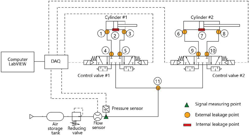
Figure 1 Schematic diagram of experiment system.

2 Experiment Setup, Data Acquisition and Pre-processing

2.1 Experiment Setup

Figure 1 shows the schematic diagram of experiment system. The system is mainly composed of two pneumatic cylinders and two 5/3 control valves. The cylinder #1 is MDBB32-200Z produced by SMC with the stroke of 200 mm. The cylinder #2 is MDBB32-400Z produced by SMC with the stroke of 400 mm. Both control valves are SY5320-5LZD-01 produced by SMC. The operations of two cylinders are controlled via two control valves. Figure 2 shows the working paces of two cylinders. That is, one cycle of operation is 4 s. The pressure reducing valve is IVT1050-211L produced by SMC and the outlet pressure is set at 0.35 MPa. The flow sensor is SFAB-600U-HQ10-2SV-M12 produced by FESTO and the pressure sensor is ISE40A-C6-R-M produced by SMC. The flowrate and pressure signals are collected via a data acquisition system and processed in LabVIEW. The sampling frequency is set at 100Hz.

In this study, leakages in 11 positions are simulated as shown in Figure 1, including 2 internal leakages of two cylinders and 9 external leakages. Hereinto, the internal leakages are simulated by artificially damaging the sealing ring of the pistons. The detailed operating conditions simulated in experiments are shown in Table 1. It should be noted that only one fault is simulated in each experiment. The main target of this study is to detect and locate the position of leakages; therefore, the leakage rates are all set at 15 L/min and 0.6 L/min for all external leakages and all internal leakages, respectively.

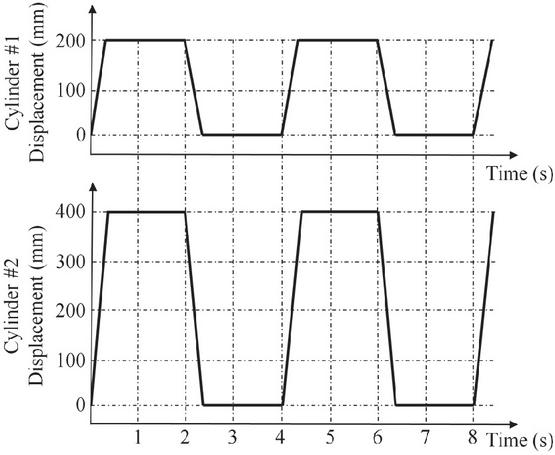
Figure 2 Working paces of two pneumatic cylinders.

Table 1 Normal and faulty conditions simulated in experiments

Operating Conditions	Degree of Leakage Fault
Normal	None
External leakage at position 1	15 L/min
Internal leakage at position 2	0.6 L/min
External leakage at position 3	15 L/min
External leakage at position 4	15 L/min
External leakage at position 5	15 L/min
External leakage at position 6	15 L/min
Internal leakage at position 7	15 L/min
External leakage at position 8	0.6 L/min
External leakage at position 9	15 L/min
External leakage at position 10	15 L/min
External leakage at position 11	15 L/min

2.2 Data Acquisition and Pre-processing

Figure 3 shows the whole process of leakage fault diagnosis designed in this study, including data acquisition and pre-processing. Each experiment under different operating conditions in Table 1 is conducted twice. The data collected in the first experiment is used for training and validation. The data collected in the independent repeated second experiment is used for testing. As shown in Table 2, for each operating condition, the number of samples in training set, validation set, and test set are 200, 10, and 40, respectively.

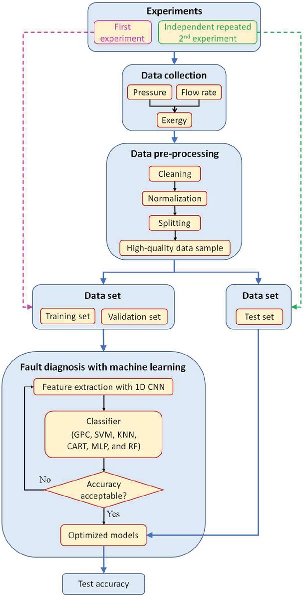
Figure 3 The whole process of leakage fault diagnosis designed in this study.

The pressure data and flowrate data in the sole signal measuring point as shown in Figure 1 is collected in this study. Besides, the exergy data is calculated with the following equation. It can be regarded as a fusion of pressure and flowrate.

{\dot{E}}_{x} = \dot{m} T_{0} R_{g} \ln \frac{p}{p_{0}}

where ${\dot{E}}_{x}$ is the exergy flowrate of compressed air with unit kJ/s, $\dot{m}$ is the mass flowrate of compressed air with unit kg/s, $R_{g}$ is the gas constant with unit J/kg/K, and $p$ is the absolute pressure of compressed air with unit Pa. $T_{0}$ and $p_{0}$ are the reference temperature and reference pressure, respectively. In this study, the pressure and temperature of atmospheric are used for the reference state and set as 101325 Pa and 25 $^{\circ}$ C, respectively. It should be noted that the influence of temperature on exergy is neglected due to the negligible fluctuation of temperature.

Table 2 Number of samples in the different data sets and labels of different operating conditions

	Number	Number	Number
	of Samples	of Samples	of Samples
Operating Conditions	in Training Set	in Validation Set	in Test Set	Label
Normal	200	10	40	0
External leakage at position 1	200	10	40	1
Internal leakage at position 2	200	10	40	2
External leakage at position 3	200	10	40	3
External leakage at position 4	200	10	40	4
External leakage at position 5	200	10	40	5
External leakage at position 6	200	10	40	6
Internal leakage at position 7	200	10	40	7
External leakage at position 8	200	10	40	8
External leakage at position 9	200	10	40	9
External leakage at position 10	200	10	40	10
External leakage at position 11	200	10	40	11

Due to the uncertainties and errors induced by sensors and experimental devices, there are generally noise, missing values, duplicates, and outliers in the collected flowrate, pressure, and calculated exergy data. The raw data is not preferred to be directly used for training machine learning models. Therefore, the data pre-processing is critical for improving diagnostic accuracy. The data quality should be improved by data cleaning and the raw data should be transformed into a format more suitable for subsequent feature extraction algorithms and machine learning models. The normalization is conducted using Python and each data sample is normalized to the interval [0, 1]. Therefore, the efficiency of training machine learning models can be enhanced.

As shown in Figure 4, it can be seen that there is obvious and regular periodicity of collected data. Thus, the time series of data can be split into cycles. Each cycle is 4 seconds (400 data points) and can be regarded as one sample used for machine learning.

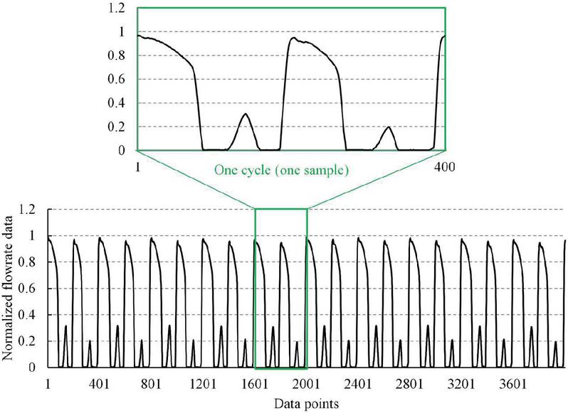
Figure 4 Time series of normalized pressure data and splitting of data samples.

3 Leakage Detection with Machine Learning

The main process of leakage fault diagnosis with machine learning is shown in Figure 3. One-dimensional convolutional neural network (1D CNN) is used for feature extraction. Six classifiers, including the Gaussian Process Classifier (GPC), Support Vector Machine (SVM), k-Nearest Neighbors (KNN), Classification and Regression Tree (CART), Multilayer Perceptron (MLP), and Random Forest (RF), are used for comparison and diagnosing the leakage faults. The detailed configures of 1D CNN and six classifiers are illustrated in Figure 5.

As shown in Figure 5, the input layer comprises 400 neurons representing the 400 data of the one sample. The first convolutional layer consists of 32 filters each with a kernel size of 3, and is employed for extracting local features from the input data. This layer operates without padding (Padding: Valid), ensuring that convolution occurs strictly within the valid boundaries of the data. The subsequent activation function, the Rectified Linear Unit (ReLU), is applied to enhance the non-linear expressive capacity of the model. The subsequent first pooling layer employs a 3 $\times$ 3 pooling kernel with a stride of 3, performing max pooling operations to reduce the dimensionality of the features, thereby lessening the complexity of subsequent computations and improving the model’s translational invariance. The second convolutional layer of the network consists of 64 filters. And other parameters are set identically with those in the first convolutional layer. The setup of the second pooling layer is the same as the first pooling layer, further reducing the feature dimensions. The flatten layer transforms the multi-dimensional feature maps into a one-dimensional vector, which is suitable for processing by the fully connected layer. The fully connected layer engages in a comprehensive connection of the flattened features and applies ReLU once again for activation. Finally, the output layer transforms the network’s outputs into a probability distribution via the Softmax activation function to facilitate classification decisions. The right side of Figure 5 lists six machine learning classification models along with their parameter configurations. The Random Forest (RF) model is set with 11 trees. The K-Nearest Neighbors (KNN) model chooses 5 nearest neighbors and a 1-norm distance metric. The Gaussian Process Classifier (GPC) employs a Radial Basis Function (RBF) kernel and a fixed random state. The Classification and Regression Tree (CART) does not limit the maximum depth of the tree and sets the minimum number of samples required for leaves and splits. The Support Vector Machine (SVM) is set with the RBF kernel, the regularization parameter is set as 10.0, and gamma value is set as 0.10. The Multi-Layer Perceptron (MLP) has finely tuned parameters such as regularization parameter, optimization algorithm, and maximum iterations.

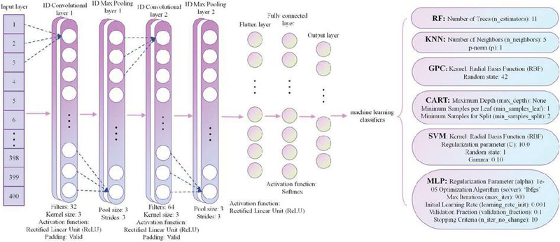
Figure 5 Detailed configurations of 1D CNN and classifiers.

One of the advantages of CNN is the ability to effectively extract features from data, while significantly reducing the number of network parameters through a shared weight mechanism, thereby effectively decreasing the risk of overfitting. Figure 6 shows the cases of loss curve for the training and validation data set of flowrate, pressure, and exergy data in one experiment. It is evident that both training and validation losses tend towards zero, indicating that the model has achieved good convergence on these datasets without overfitting. The result indicates the efficiency and reliability of CNN in this study.

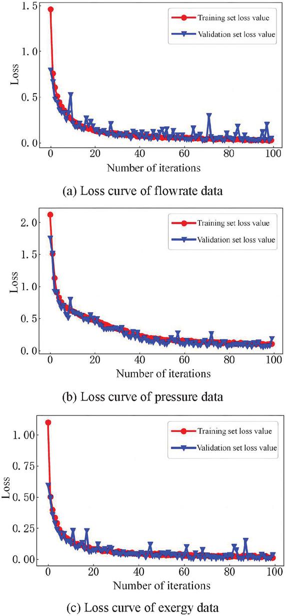
Figure 6 Cases of loss curve in one experiment.

4 Results and Discussions

In this section, the diagnostic results of all experiments are presented and compared. Confusion matrix analysis and Class Activation Mapping (CAM) are used for analysing and interpreting the results.

4.1 Diagnostic Accuracy of Various Classifiers

Table 3 shows the detailed diagnostic accuracy of all tests. For each classifier and each signal, ten times of tests are conducted. Then the average accuracy of these ten tests is calculated and regarded as the index for evaluating the diagnostic performance of the machine learning models. Figure 7 shows the intuitional comparison of various machine learning models. It should be noted that, in the training processes of these models, an accuracy of 85% is accepted as the threshold value for confirming the optimized models. There are two reasons for this moderate threshold. The first is to save the time of training and optimizing models. The second reason is to consider that this study is a theoretical feasibility validation more than a practical industrial application. Therefore, the test results presented in Table 3 and Figure 7 are not optimal. Nevertheless, they are sufficient to indicate and compare the performance of various machine learning models under identical conditions.

From Figure 7, it is evident that five classifiers (GPC, SVM, KNN, CART, and RF) present better performance than MLP classifier. In terms of five better classifiers, the diagnostic accuracies based on flowrate data and exergy data exhibit higher values than those based on pressure data. Besides, the diagnostic accuracies based on exergy data show slightly higher values than those based on flowrate data. This is mainly because the exergy is the fusion of flowrate and pressure. This is consistent with the results revealed in reference [2]. It should be noted that this does not mean that the pressure data cannot be used for effective fault diagnosis in pneumatic systems. It can only prove that pressure data performs not well enough in this specific system. Overall, this study verifies the feasibility of detecting and locating the multipoint leakages in a pneumatic system by analysing signal measured at a sole upstream point with the help of machine learning methods.

Table 3 Detailed diagnostic accuracy of all tests

		Accuracy of Ten Tests										Average
Classifiers	Signals	1	2	3	4	5	6	7	8	9	10	Accuracy
GPC	Flowrate	89.79%	84.58%	86.67%	86.67%	86.25%	85.63%	82.08%	88.96%	89.17%	87.92%	86.77%
	Pressure	87.50%	77.71%	88.96%	83.13%	70.42%	68.33%	84.79%	85.42%	73.75%	60.42%	78.04%
	Exergy	85.42%	86.88%	90.00%	90.00%	88.33%	98.30%	85.00%	88.13%	88.13%	88.75%	88.15%
SVM	Flowrate	89.79%	83.96%	86.88%	88.33%	86.67%	85.42%	82.29%	89.58%	89.79%	88.96%	87.17%
	Pressure	87.71%	61.25%	88.13%	83.54%	70.00%	68.75%	84.38%	85.00%	74.79%	85.00%	78.85%
	Exergy	86.67%	88.75%	90.00%	96.30%	94.20%	91.04%	87.29%	92.71%	88.75%	88.54%	89.48%
KNN	Flowrate	89.38%	84.58%	8708%	87.92%	85.63%	85.63%	82.50%	89.58%	89.17%	87.50%	86.90%
	Pressure	86.67%	84.58%	87.29%	84.38%	70.42%	68.96%	83.54%	85.63%	73.96%	61.88%	78.73%
	Exergy	87.50%	86.46%	94.20%	96.30%	88.54%	98.30%	86.04%	91.88%	87.29%	88.54%	88.81%
CART	Flowrate	92.10%	83.96%	85.83%	87.29%	85.21%	85.83%	81.67%	91.25%	94.20%	86.04%	86.77%
	Pressure	87.50%	87.29%	89.17%	82.71%	69.17%	67.92%	85.83%	86.67%	75.83%	59.17%	79.13%
	Exergy	87.08%	86.46%	91.04%	88.54%	89.17%	98.30%	83.54%	89.38%	85.42%	93.13%	88.46%
MLP	Flowrate	49.17%	43.96%	45.83%	45.00%	48.54%	48.33%	43.33%	55.83%	50.00%	49.38%	47.94%
	Pressure	67.92%	53.33%	57.29%	73.96%	67.50%	40.63%	57.50%	55.00%	47.71%	42.08%	56.29%
	Exergy	37.50%	46.04%	58.13%	48.96%	46.25%	46.67%	44.17%	78.13%	46.25%	51.04%	53.10%
RF	Flowrate	92.10%	84.38%	86.88%	84.38%	85.21%	85.63%	82.50%	88.33%	87.29%	87.92%	86.27%
	Pressure	86.46%	85.00%	87.29%	83.13%	69.58%	68.96%	85.83%	87.50%	76.04%	58.75%	78.85%
	Exergy	86.04%	86.46%	90.00%	90.00%	89.17%	98.30%	84.58%	91.67%	87.71%	88.75%	88.52%

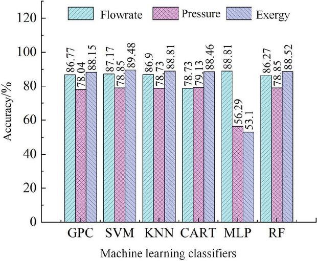
Figure 7 Average accuracy of various machine learning methods.

4.2 Confusion Matrix Analysis and Class Activation Mapping

Confusion matrix analysis and Class Activation Mapping (CAM) are two important methods for understanding, interpreting and optimizing machine learning models. In this subsection, the results presented in subsection 4.1 are analysed and discussed using these two methods.

4.2.1 Confusion matrix analysis

The confusion matrix is a tool used to assess the detailed performance of classification models, especially in the context of multi-class classification problems. It provides insight into the classification ability of the model by comparing the predicted results with actual results. Each value in the matrix represents the number of samples from a specific category that have been misclassified into each incorrect category. In this study, confusion matrix analysis reveals classification confusion among different leakage locations.

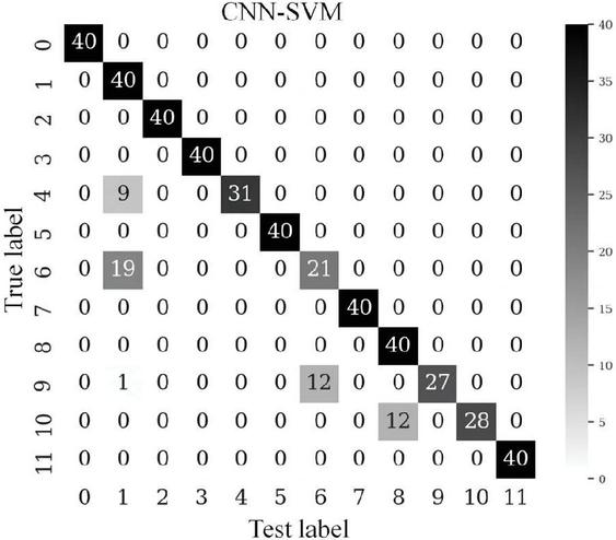
Figure 8 SVM confusion matrix for flowrate signal in the 10th test.

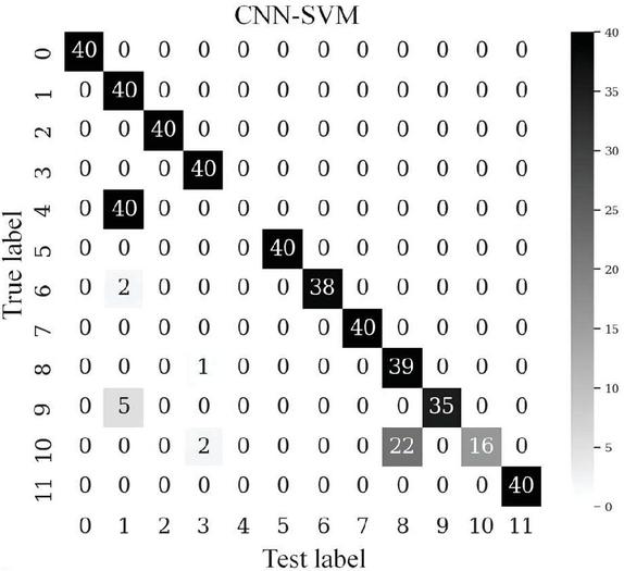
Figure 9 SVM confusion matrix for pressure signal in the 10th test.

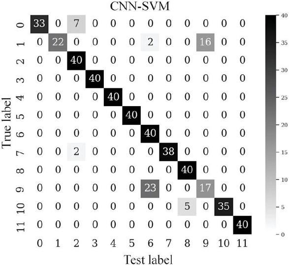
Figure 10 SVM confusion matrix for exergy signal in the 10th test.

Figures 8, 9, and 10 show the confusion matrixes in the 10th test based on the CNN+SVM model for flowrate data, pressure data, and exergy data, respectively. The serial numbers of labels are corresponding to the labels in Table 2. It is obvious that there are significant classification confusions between certain various leakage positions. Taking Figure 8 as an example, nine samples with label 4 (external leakage at position 4) are misdiagnosed as samples with label 1 (external leakage at position 1). Nineteen samples with label 6 (external leakage at position 6) are misdiagnosed as samples with label 1 (external leakage at position 1). Twelve samples with label 9 (external leakage at position 9) are misdiagnosed as samples with label 6 (external leakage at position 6). Twelve samples with label 10 (external leakage at position 10) are misdiagnosed as samples with label 8 (external leakage at position 8). The remaining 427 samples are classified correctly. It should be noted that all 40 samples with label 4 (external leakage at position 4) are misdiagnosed as samples with label 1 (external leakage at position 1) in Figure 9. Therefore, the results of confusion matrix analysis clearly illustrate the diagnostic results of each sample. As a result, in the following subsection, the Class Activation Mapping (CAM) method is utilized for visualizing the reasons why these confusions happen.

4.2.2 CAM analysis

(1) CAM analysis of flowrate data

CAM is a visualization technique that reveals the areas of the image or parts of the sequence that convolutional neural networks focus on when making classification decisions. As shown in Figure 11, the higher the value, more attention is given. By applying CAM, we can visually see the specific areas the model focuses on during classification, especially when classification errors occur. This helps us identify features that the model may misinterpret, thus providing clues for improving feature extraction strategies and adjusting the model structure.

Figure 11 shows an example of confusion between samples with label 6 and samples with label 9 as illustrated in Figure 8. Twelve samples with label 9 (external leakage at position 9) are misdiagnosed as samples with label 6 (external leakage at position 6). Only one sample is chosen as an example for interpreting the results. Figure 11(a) shows the CAM of a sample with the actual label of 6. Figure 11(b) shows the CAM of a sample with the actual label 9. While Figure 11(c) shows the CAM of a sample with the predicted label 6 which should be the actual label 9. Figure 11(d) shows the original profiles of these three samples. It is evident that they are almost the same. Therefore, the corresponding CAMs are almost the same for samples with label 6 and samples with label 9, thereby resulting in the confusion between these two operating conditions.

Another confusing issue is the high attention areas on the class activation maps. From Figures 11(a), (b), and (c), it is clear that the dominant attentions are given to the bottom flat regions of these three curves. However, from Figure 11(d) and the perspective of human intuition, it looks like more attention should be given to the top peak regions where relatively evident differences are. This is because all 12 operating conditions, instead of only two conditions, are comprehensively considered when training the machine learning models. Nevertheless, this also suggests the model could still be further improved with more complex feature extraction mechanisms to more accurately differentiate the features of different leaks. Overall, CAM provides valuable insights into the decision-making processes, thereby optimizing the machine learning models.

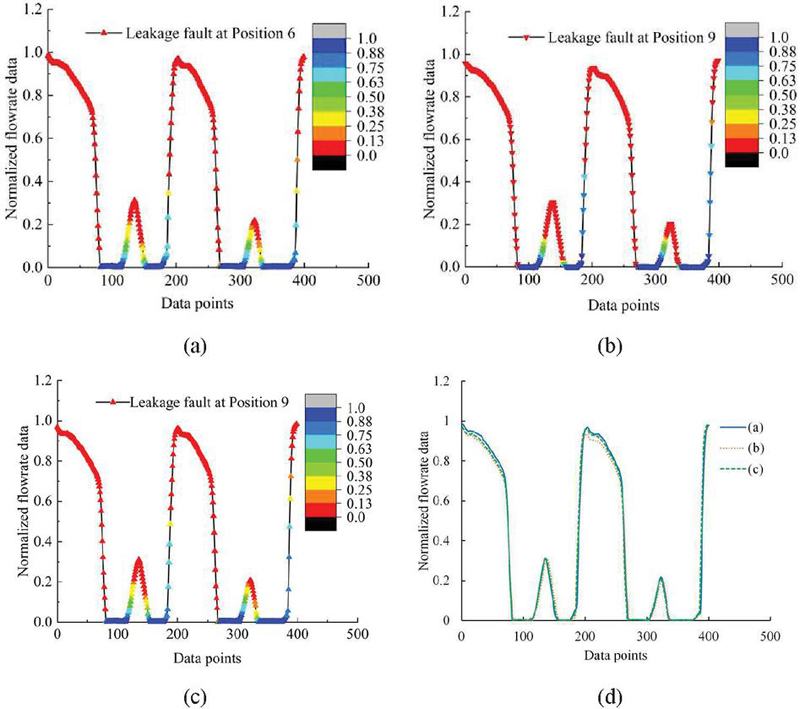
Figure 11 Class activation mapping of flowrate data of leakage at position 6 and leakage at position 9.

(2) CAM analysis of pressure data

Figure 12 shows a case of confusion of pressure data between sample with label 1 and sample with label 4. Figure 12(a) shows the CAM of a sample with the actual label of 1. Figure 12(b) shows the CAM of a sample with the actual label 4. While Figure 12(c) shows the CAM of a sample with the predicted label 1 which should be the actual label 4. Figure 12(d) shows the original profiles of these three samples. It is also evident that they are almost the same. Therefore, the corresponding CAMs are almost the same for samples with label 1 and samples with label 4, thereby resulting in the confusion between these two operating conditions. From Figure 12(d), it can be found that there is a tiny phase difference between the original profile of sample with label 1 and the original profile of sample with label 4. This reveals there is a mistake when splitting the original data. This should be corrected in following optimizations.

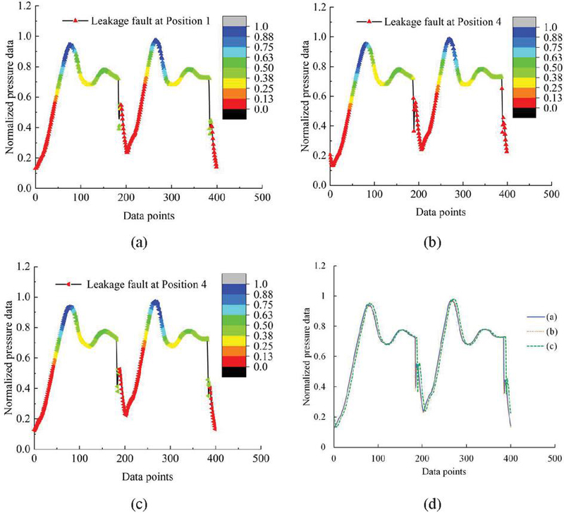
Figure 12 Class activation mapping of pressure data of leakage at position 1 and leakage at position 4.

(3) CAM analysis of exergy data

Figure 13 shows a case of confusion of exergy data between sample with label 8 and sample with label 10. Figure 13(a) shows the CAM of a sample with the actual label of 8. Figure 13(b) shows the CAM of a sample with the actual label 10. While Figure 13(c) shows the CAM of a sample with the predicted label 8 which should be the actual label 10. Figure 13(d) shows the original profiles of these three samples. It is also evident that they are almost the same. Therefore, the corresponding CAMs are almost the same for samples with label 8 and samples with label 10, thereby resulting in the confusion between these two operating conditions.

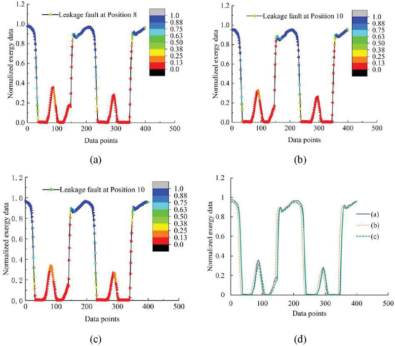
Figure 13 Class activation mapping of pressure data of leakage at position 8 and leakage at position 10.

5 Conclusions

The effective faults diagnose of multi-actuator system with simple and low-cost methods are significant for intelligent management of industrial pneumatic systems. In this study, a double-cylinder pneumatic system and leakage fault are taken as examples. Both internal and external leakages are considered. A 1D CNN is used for feature extraction. Various machine learning classifiers, including GPC, SVM, KNN, CART, MLP, and RF, are used for classifications. Overall, the results show that it is feasible to detect and locate leakages at 11 positions in the investigated pneumatic system with only one sensor upstream. The confusion matrix analysis and CAM are used for analysing the detailed performance of optimized machine learning models. The results provide valuable insights for understanding, interpreting and optimizing machine learning models. It is very interesting that the tiny internal leakages can also be identified correctly. Thus, machine learning could play a significant role in low-cost and intelligent fault diagnose in complex pneumatic systems.

Acknowledgements

This work was supported by the National Natural Science Foundation of China under Grant [number 51905066, 62103072].

References

[1] Borg M, Refalo P, Francalanza E. Failure Detection Techniques on the Demand Side of Smart and Sustainable Compressed Air Systems: A Systematic Review. Energies 2023; 16(7): 3188.

[2] Wang Z, Yang B, Ma Q, Wang H, Carriveau R, Ting DSK, Xiong W. Facilitating Energy Monitoring and Fault Diagnosis of Pneumatic Cylinders with Exergy and Machine Learning. International Journal of Fluid Power 2023; 24(4): 643–682.

[3] Li X. Intelligent fault detection and diagnosis of mechanical-pneumatic systems. PhD Thesis, Stony Brook University, 2005.

[4] Zhang K. Fault Detection and Diagnosis for Multi-Actuator Pneumatic Systems. PhD Thesis, Stony Brook University, 2011.

[5] Abela K, Refalo P, Francalanza E. Analysis of pneumatic parameters to identify leakages and faults on the demand side of a compressed air system. Cleaner Engineering and Technology 2022; 6: 100355.

[6] Gauchel W, Streichert T, Wilhelm Y. Predictive maintenance with a minimum of sensors using pneumatic clamps as an example. The 12th International Fluid Power Conference, October 12–14, 2020, Dresden, Germany.

[7] Kovacs T, Ko A. Monitoring Pneumatic Actuators’ Behavior Using Real-World Data Set. SN Computer Science 2020, 1: 196.

[8] Britzger M, Beckmann N, Seehausen F. Machine Learning Driven Local Assignment of Compressed Air Consumption Anomalies. The 13th International Fluid Power Conference, June 13–15, 2022, Aachen, Germany.

[9] Wang Z, Zhu H, Xiong W. Low-cost Fault Diagnosis of Pneumatic Systems with Exergy and Machine Learning: Concept, Verification, and Interpretation. JFPS International Journal of Fluid Power System 2023, 16(2): 24–32.

[10] Wang T, Wang X, Hong M. Gas Leak Location Detection Based on Data Fusion with Time Difference of Arrival and Energy Decay Using an Ultrasonic Sensor Array. Sensors 2018, 18(9):2985.

Biographies

Chunpu Zhang received the bachelor’s degree in Mechanical Engineering from Dezhou University in 2022. He is now pursing the master’s degree in Mechanical Engineering in Dalian Maritime University. His research areas include data-driven modelling, fault diagnosis of pneumatics, and machine learning.

Zhiwen Wang received the bachelor’s degree of Marine Engineering from Dalian Maritime University in 2012 and the philosophy of doctorate degree in Marine Engineering from Dalian Maritime University in 2018, respectively. He is currently working as an Associate Professor at the Department of Mechanical Engineering, Dalian Maritime University. His research areas include energy saving and FDD of pneumatics, thermodynamics, and energy storage.

Lingchao Yu received his bachelor’s degree in Mechanical Engineering from Qingdao University of Science and Technology in 2023. Currently, he is pursuing his master’s degree in Mechanical Engineering at Dalian Maritime University. His research interests include pneumatic fault diagnosis and machine learning.

Zheng Zhao received his B.S. degree from Dalian University of Technology in 2010. He received his M.S. and Ph.D. degree from Zhengzhou Science and Technology Institute in 2013 and 2017. Now he is working at College of Artificial Intelligence, Dalian Maritime University. His research interests include artificial intelligence security, network security, and deep learning applications.

Fei Wang is currently a lecturer in college of Information Science and Technology at Dalian Maritime University of China. He received the Ph.D. degree in Control Theory and Engineering from the Dalian University of Technology, P. R. China in 2019. He obtained the B.Sc. and M.Sc. degrees in Computer Science and Technology from Dalian Maritime University, P. R. China, in 2012 and 2015 respectively. His research interests include robotics, deep learning, 3d data processing, and semantic scene understanding.

Wei Xiong is a Professor of Mechanical Engineering, Dalian Maritime University. He is the director of Ship Electromechanical Equipment Institute. He received his PhD in the Faculty of Mechatronic Engineering from Harbin Institute of Technology, China. His major research interests are fluid power and control, marine rescue, and compressed air energy storage.