Thermal-fluid Optimization Model of Small-scale Hydraulic Conduits
Jeffrey Bies* and William Durfee
Mechanical Engineering, University of Minnesota, Minneapolis, MN, United States
E-mail: bies0040@umn.edu
*Corresponding Author
Received 11 May 2024; Accepted 16 May 2024
Abstract
Multiphysics topology optimization has applications in computer-aided design of products, including small-scale fluid power systems where flow efficiency, thermal management, and weight management matter. While algorithms exist that can optimize a single objective, there are no solutions that can simultaneously address all three of these factors. This study developed a multiphysics topology optimization process that uses a thermal-fluid-structure model to generate high-pressure hydraulic designs where passive cooling is built into the flow channels. Python was used with Open-Source Field Operation and Manipulation (OpenFOAM) for geometry creation, meshing, and finite volume and sensitivity analysis to implement the multi-objective optimization for small-scale fluid power systems. The process was performed iteratively to inform the next iteration’s geometry until an optimized design was reached.
The results show that pressure drop, fluid density, fluid velocity, and inlet diameter are positively correlated with capillary branching and that design space and viscosity are negatively correlated with capillary branching. Enhanced heat transfer came at the cost of pressure drop, where increasing the allowable pressure drop by 195% led to an increased temperature drop of 17%. Expanding the design space had the most significant impact on heat transfer, where extending the design space width by three times led to a 365% increase in temperature drop. Incorporating a curved exterior wall in the design space while holding the area and mesh node count constant led to a 3% increase in temperature drop while decreasing computational time by 68%. Lower viscosity of the working fluid leads to increased capillary branching with minimal impact on temperature drop (0.3%), while incorporating a temperature-dependent viscosity model led to a more prominent temperature drop (15%). Future work will expand the topology optimization method to incorporate structural optimization to handle load-bearing.
Keywords: Continuous adjoint method, hydraulic, multi-objective optimization, OpenFOAM, topology optimization.
1 Introduction
Hydraulics can deliver high force and power through flexible hoses while maintaining control through fluid incompressibility [1]. While small-scale hydraulics has applications in areas such as wearable exoskeletons and mobile robotics, it also introduces challenges with regard to efficiency, thermal management, and system weight. Thermal-fluid topology optimization is ideal for addressing these concerns by creating branched capillaries with highly efficient flow paths to reduce the temperature of the fluid and, therefore, minimize risk of injury or discomfort on the wearer of the exoskeleton [2]. This will also minimize weight because higher fluid flow efficiency allows for a smaller battery to deliver the same amount of usable energy.
There are several classifications of optimization; however, the two most widely used types are shape and topology optimization [2–6]. Shape optimization is ideal for cases where the general shape is fixed, as is the case for an airfoil where the shape is parameterized into features such as size, angle, and contour [7]. Parameterization can significantly reduce the design variables needed to optimize and, therefore, decrease computation time; however, it is not capable of adding or removing features that were not predefined. In cases where the optimal shape is unknown, topology optimization is ideal because every element within the design space can be altered in terms of the presence or absence of the allowable material(s). Element-wise control allows design features to be added or removed as needed by the optimization process [8]. While topology optimization offers greater freedom of design, it significantly increases the computational demand from the order of hundreds of variables or less to thousands or even millions of variables, depending on the size of the design space. Traditional optimization strategies of adjusting variables one at a time become impossible to use for topology optimization with present-day computational capabilities.
The continuous adjoint method makes topology optimization feasible for large design spaces by reducing the number of iterations required to evaluate variable sensitivity from potentially millions to only two iterations. The first iteration solves for the governing equations relevant to the design goals, while the second iteration solves for the gradient of the governing equations within the design space. This combination allows the algorithm to map out the sensitivity of design space and adjust the design such that the optimization goal is minimized or maximized. Since the sensitivity will change as the design changes, this process needs to be repeated until the solution converges on a local optimum.
Optimization has led to significant improvements to designs with single objectives based on structural mechanics, fluid mechanics, or heat transfer; however, there has been little work done to couple these areas of physics [9–11]. Most advances in multiphysics optimization have been within the last six years, with the earliest work published in 2010 [12].
The work of Yu et al. offers the closest link to the research presented here with the design of a heat sink; however, the goal of the study involved cooling the design space rather than cooling the fluid [13]. Their design space and fluid properties were also fixed, and the inlet temperature was set to absolute zero. The most fundamental change to the program used was the handling of the pressure drop. The work of Yu et al. focused on the power dissipation defined at the inlet and outlet only, whereas the current study defined power dissipation across the entire geometry, which is the preferred definition used for continuous adjoint method because it provides more information about where in the geometry the pressure is being lost and how to adjust the design accordingly through sensitivity analysis [14]. It is also worth noting that this study is a steppingstone towards incorporating an algorithm that optimizes thermal, fluid, and structural considerations with additional processing to prepare it for manufacturing.
This paper introduces a computational pipeline that incorporates several applications to achieve multiphysics topology optimization. Then the steps of the adjoint optimization algorithm are described. Next, the impact of design space, viscosity, and allowable pressure drop are explored to determine their effects on the resulting optimized designs. The conclusions of the design guidelines are discussed, and the future directions of this research are addressed.
2 Materials and Methods
2.1 Automated Optimization Pipeline Overview
OpenFOAM Foundation v9 was used as the computational fluid dynamics (CFD) software to handle solving the governing and adjoint equations. While OpenFOAM has extensive custom solver capabilities, mesh control and post-processing capabilities are limited. Therefore, a pipeline was created that uses Python to connect OpenFOAM to existing specialized software to automate the optimization process (Figure 1). The specialized software packages for mesh generation, post-processing, and computer-aided design (CAD) were Gmsh, ParaView, and Open Cascade, respectively.
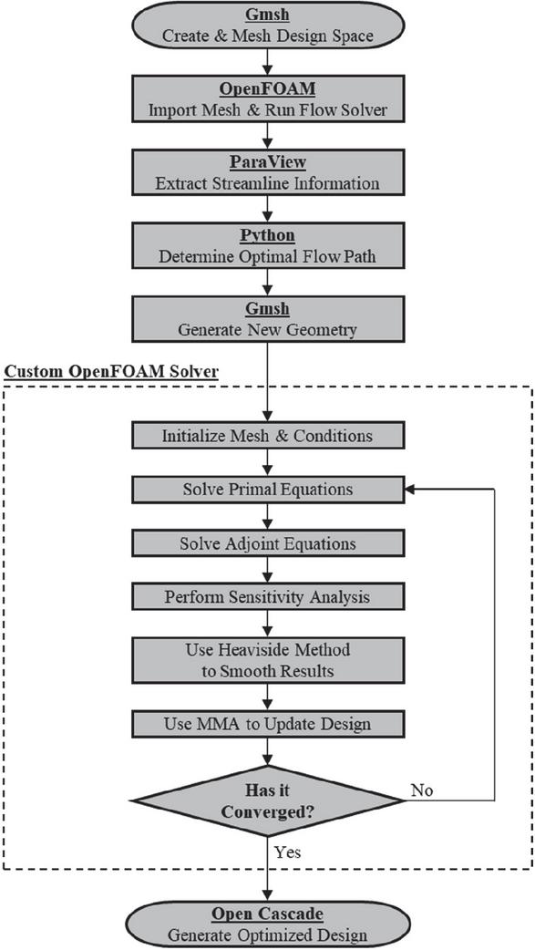
Figure 1 Pipeline overview diagram.
2.2 Design Space
The two-dimensional design space constructed and meshed using Gmsh comprises the inlet and outlet at the left and right extreme of Figure 2, respectively, and the optimization region between them. The inlet and outlet have the material within this region fixed as a fluid. The optimization region is made of a porous material with a pseudo density prescribed to transition between fluid () and solid (). Initially, this porous region is set to a uniform intermediate pseudo density equal to the target fluid volume percentage of the final design. As the optimization algorithm operates on the design space, this porous region will asymptotically converge towards fluid or solid in areas where it is needed as dictated by the design goals.
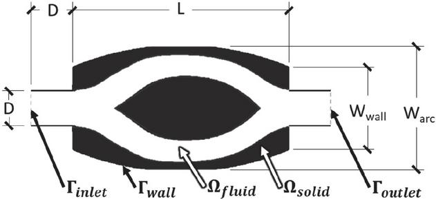
Figure 2 Design space dimensions and domain and boundary definitions.
2.3 Primal Equations
This study explores low Reynolds number cases () where a laminar, steady-state, incompressible model was chosen. While most material properties were assumed independent of temperature, the impact of temperature on viscosity was explored due to the high temperature dependence of the chosen fluid’s viscosity. Additionally, the effects of viscous dissipation on heat generation were not considered.
For fluid flow, Navier-Stokes equations were used to derive the domain conditions with (1) and (2) where , , , and correspond respectively to the fluid’s velocity, density, pressure, and viscosity [14].
| (1) | |
| (2) |
The body force is prescribed to this fluid by (3) as an artificial friction force created by the porous media to slow the fluid’s velocity as the media converges on being solid while allowing free flow when the media converges on being fluid [15].
| (3) |
The inverse of the local permeability controls how much resistance the fluid will experience based upon the pseudo density by using the Rational Approximation of Material Properties (RAMP) function [16]
| (4) |
where is a relatively large number tuned to prevent flow when the material is solid (). The RAMP shape factor is used to determine how quickly goes from 0 to based upon the pseudo density. In this study, and were set to and 0.005, respectively, based upon previous work [13]. As the optimization iterations progress, the value of increases incrementally until it reaches 0.01, which creates a sharper transition between solid and fluid.
For conjugate heat transfer, the energy equation provides the domain conditions for thermal conduction in the solid domain and thermal convection in the fluid domain with
| (5) | |
| (6) |
respectively, where is the temperature, is the prescribed heat generation, is the fluid’s heat capacity, and and are the fluid and solid thermal conductivity, respectively [17].
In order to accommodate the porous media, a unified equation was created to translate between the solid and fluid domain based upon the pseudo density. This can be done by implementing the RAMP function into thermal conductivity and making the thermal transport and heat generation a function of , resulting in
| (7) |
where,
| (8) |
At the inlet , the temperature and velocity were prescribed, and the pressure was set as a zero gradient. At the outlet , the outlet pressure was prescribed by the operating pressure, and the temperature and velocity conditions were set to zero gradient. All other boundaries of the domain were treated as a wall with a no-slip, adiabatic condition and a zero-gradient pressure.
2.4 Adjoint Equations
The second stage of the thermal-fluid optimization solver involves solving for the adjoint equations, which are analogous to a gradient of the primal equations with respect to the variables of interest (i.e., velocity, temperature, and pressure). The resulting adjoint equations, derived in [13], can be given by
| (9) | |
| (10) | |
| (11) |
where , , and are Lagrange multipliers (commonly known as adjoint variables) with units that are inverse to the corresponding variables.
Since the adjoint equations need to be solved in the same manner as the primal equations, boundary conditions also need to be established for the adjoint variables. While most of the adjoint variable boundary conditions match the ones prescribed for their counterparts, a few conditions at the inlet and outlet need to be adjusted. At inlet, and . The boundary conditions for the outlet need to be solved for each of the adjoint variables using
| (12) | ||
| (13) |
where corresponds to the surface normal.
2.5 Optimization Goal
The primary goal function of this optimization is to minimize the average temperature at the outlet, which can be characterized by
| (14) |
2.6 Sensitivity Analysis
The power dissipation was set as a constraint with an adjustable target rather than a goal to be minimized so that the optimal heat dissipation could be explored as a function of allowable pressure drop. Power dissipation was chosen as a constraint as opposed to the pressure drop because volume integrals work better for topology-based adjoint solvers because it allows for the formulation of a sensitivity as a function of density across the entire domain .
| (15) |
To minimize the temperature at the outlet, the thermal adjoint equation given by (11) needs to be differentiated by the pseudo density to obtain
| (16) |
2.7 Smoothing and Updating Results
To improve the mesh-dependent stability of the solver and smooth the optimized solution, a density filter was implemented based on the Helmholtz Partial Differential Equation (PDE) filter [18]
| (17) |
where is the original pseudo density with the lower bound extended linearly from 0 to 1, is the prescribed filter radius, and is the filtered pseudo density. The filtered pseudo density is then regularized using the Heaviside function:
| (18) |
where is an adjustable parameter tuned to control the transition bandwidth. To facilitate the sensitivity analysis, filtering process, and the resulting design space update, the Method of Moving Asymptotes first proposed by [19] and linked to OpenFOAM via the Portable, Extensible Toolkit for Scientific Computation (PETSc) framework written by [20] was used.
2.8 Case Studies
The case studies in this paper explored variations in allowable pressure drop, design space, and viscosity while holding all other variables constant. The hydraulic fluid used was ISO Grade 70 mineral oil with an operating pressure of 6.89 MPa (1 kpsi). The fluid enters the 2-mm diameter () inlet at 353.15 K and 0.45 m/s. The solid region is aluminum with a heat sink of and a minimum temperature of 293.15 K.
Since the inlet and outlet correspond to a straight pipe, the initial run through the OpenFOAM incompressible flow solver (simpleFoam) is only used to determine the reference power dissipation rather than creating a new design space based upon the optimal flow path. This reference point of m s was used to determine the allowable power dissipation for the case studies as shown in Table 1 in the order they will be presented and discussed. The case conditions began with a control case with each parameter (power dissipation, design space width, and kinematic viscosity) set to a mid-range value that subsequent cases could be referenced from. Cases A through H generally increase or decrease one parameter by 50% from the control’s reference point, while the remaining two parameters are unchanged. Cases A and B represent changes in power dissipation, C through E correspond to changes in design space, and F through H alter kinematic viscosity.
Table 1 Case conditions
| Power | Design | Kinematic | |
| Case | Dissipation () | Space Width () | Viscosity |
| Control | 10 | 10 | 60 |
| A | 5 | 10 | 60 |
| B | 15 | 10 | 60 |
| C | 10 | 5 | 60 |
| D | 10 | 15 | 60 |
| E | 10 | 4 | 60 |
| F | 10 | 10 | 30 |
| G | 10 | 10 | 90 |
| H | 10 | 10 | TD |
While the design space length was fixed at 10 , the design space width was allowed to vary between 5 and 15 , with Case E taking the smallest design space and adding an arc width of 6 while maintaining approximately the same overall area as Case C. A structured grid mesh with a face size of 0.025 mm was applied for all design spaces.
The kinematic viscosity was varied between 30 and 90 corresponding to the low and high end of the expected range for ISO Grade 70 Mineral Oil with Case H incorporating a temperature dependence for the viscosity.
3 Results and Discussion
The first case acted as the control from which the following cases would be compared, where all of the variables were set at the mid-point of their respective ranges. The region above the symmetry line of Figure 3 represents how the fluid and solid regions formed within the design space. The largest channel makes a steep angle with the symmetry line before returning to the outlet. Smaller capillaries can also be seen connecting to the main channel at three points and meeting towards the center of the design space.
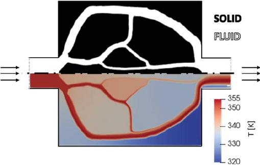
Figure 3 Optimization results for the control case.
The region below the symmetry line of Figure 3 shows the thermal variation across the design space, with the hottest (red) area at the inlet and along the center of the widest channel of the fluid region. The coldest (blue) areas of the design space are found in the solid region due to the negative heat flux prescribed there, with warmer areas located in the regions of high capillary density. The outlet has a non-uniform temperature gradient resulting in a temperature drop of 8.4 K (Table 2).
Table 2 Case results summary
| Pressure | Temperature | Computational | |
| Drop (m s) | Drop (K) | Iterations () | |
| Control | 22.4 | 8.4 | 191 |
| A | 11.2 | 7.6 | 172 |
| B | 32.9 | 8.9 | 189 |
| C | 22.0 | 2.2 | 980 |
| D | 24.4 | 10.4 | 185 |
| E | 19.2 | 2.3 | 311 |
| F | 19.4 | 8.5 | 197 |
| G | 21.5 | 8.5 | 199 |
| H | 22.2 | 9.7 | 179 |
| The average iteration was 48.6 seconds on a single Intel i7 processor. | |||
3.1 Pressure Drop
As the allowable pressure drop increases, this allows for increased branching in the flow path, which results in greater heat dissipation for the fluid (Figure 4) As is shown in Figure 4, Case A, if the allowable pressure drop is low enough, all capillary features will disappear with the eventual limit of becoming a straight pipe. In this case, a temperature drop increase of 17% came at the cost of increasing the pressure drop by 195%.
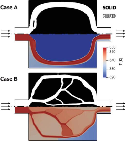
Figure 4 Optimization results comparing low pressure drop (Case A) and high pressure drop (Case B).
It should be noted that Cases C through E were set to a constant power dissipation; however, variations in pressure drop were measured. This can be attributed to the balance between converging temperature drop and pressure drop where, depending on the design goal, full convergence for one parameter may not be achievable. The trade-off between pressure drop and heat dissipation has consequences for optimized design when thermal maintenance and fluid power efficiency are critical.
3.2 Design Space
The definition of the design space has the most impact on the optimized results. As shown in Figure 5, Case D, the main channel will always reach as far as possible toward the boundary of the design space, no matter how large that space gets. In contrast, Figure 5, Case C, demonstrates that too small a design space will lead to capillary branching with increased thermal uniformity. While the smaller design space may be more desirable depending on design constraints, it comes at the cost of heat dissipation. Expanding the design space by three times results in an increased temperature drop of 365%, indicating that the largest allowable design space is desirable for heat transfer.
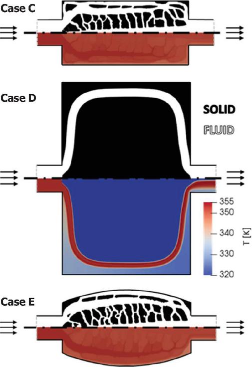
Figure 5 Optimization results for varying domain size and shape with a domain width at 50% of the control (Case C) and 150% of the control (Case D) as well as incorporating an arc with the same area as the top design (Case E).
Another implication of small design spaces is that the computational time was significantly higher (4x) than for all of the other cases explored. Comparing Figure 5, Cases C to E, the general structure remained similar but removed the capillary branches that reached the corners of the design space. The inclusion of a curved domain space led to a modest improvement in heat transfer of 3% while reducing the computational time by 68%.
3.3 Viscosity
While the impact of temperature-independent viscosity on heat dissipation was negligible, it provides insights into the shape of the optimized fluid path. In Figure 6, Case F, the low viscosity allows for more branching and creates a more jagged design than is seen in Figure 6, Case G. These features are combined when the viscosity is allowed to vary with temperature. In Figure 6, Case H, the dispersion angle is more significant as is seen with low viscosities; however, as the fluid is allowed to cool, the branching becomes smoother and evenly spaced. The result of incorporating temperature-dependent viscosity is an increase in temperature drop of 15%, which highlights the importance of performing optimization with temperature-dependent material properties. While this section discusses the impacts of viscosity, the non-dimensional behavior of fluid through the Reynolds number allows the inverse guidelines to be made about density, velocity, and inlet diameter, where increasing any of these will lead to a higher Reynolds number and, therefore, more jagged branching as seen in Figure 6, Case F.
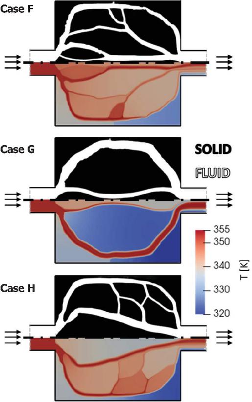
Figure 6 Optimization results for varying viscosity with low viscosity (Case F), high viscosity (Case G), and temperature-dependent viscosity (Case H).
4 Conclusion
The authors introduced a thermal-fluid optimization algorithm to explore the implications of pressure drop, design space, and viscosity. This study shows that increasing pressure drop, fluid density, fluid velocity, and inlet diameter or reducing design space and viscosity led to increased capillary branching with more extreme and jagged flow paths. Increasing heat transfer significantly increases the pressure drop. Design space had the most significant impact on heat dissipation, where tripling the design space resulted in a 395% increase in temperature drop. Curving the design space led to a computational reduction of 68% with modestly enhanced heat transfer. Incorporating temperature-dependent viscosity led to a 15% increase in temperature drop. Future work will expand the capabilities of the program by incorporating a structural optimization component for load-bearing scenarios and prepare the optimized design for different manufacturing scenarios, including additive manufacturing and traditional methods of manufacturing.
References
[1] W. Durfee, J. Xia and E. Hsiao-Wecksler, “Tiny hydraulics for powered orthotics,” 2011 IEEE International Conference on Rehabilitation Robotics, pp. 1–6, 2011.
[2] J. P. Leiva, “Freeform optimization: a new capability to perform grid by grid shape optimization of structures,” in 6th China-Japan-Korea Joint Symposium on Optimization of Structural and Mechanical Systems, Kyoto, Japan, 2010.
[3] J. P. Leiva, “Methods for generation perturbation vectors for topography optimization of structrures,” in 5th World Congress of Structural and Multidisciplinary Analysis and Optimization, Lido di Jesolo, Italy, 2003.
[4] J. P. Leiva, “Topometry optimization: a new capability to perform element by element sizing optimization of structures,” in 10th AIAA/ISSMO Symposium on Multidisciplinary Analysis and Optimization, Albany, New York, United States of America, 2004.
[5] J. P. Leiva and B. C. Watson, “Shape optimization in the genesis program,” in Optimization in Industry II, Banff, Canada, 1999.
[6] J. P. Leiva, B. C. Wattson and I. Kosaka, “Modern structural optimization concepts applied to topology optimization,” in 40th Structures, Structural Dynamics, and Materials Conference and Exhibit, St. Louis, Missouri, United States of America, 1999.
[7] G. Halila, J. Martins and K. Fidkowski, “Adjoint-based aerodynamic shape optimization including transition to turbulence effects,” Aerospace Science and Technology, vol. 107, 2020.
[8] G. Rozvany, “Aims, scope, methods, history and unified terminology of computer-aided topology optimization in structural mechanics,” Structural and Multidisciplinary Optimization, vol. 21, no. 2, pp. 90–108, 2001.
[9] Y. J. Lee, P. S. Lee and S. K. Chou, “Enhanced thermal transport in microhcannel using oblique fins,” Journal of Heat Transfer, vol. 134, no. 10, pp. 1–10, 2012.
[10] Y. Sui, C. J. Teo, P. S. Lee, Y. T. Chew and C. Shu, “Fluid flow and heat transfer in wavy microchannels,” International Journal of Heat and Mass Transfer, vol. 53, no. 1, pp. 2760–2772, 2010.
[11] Z. Lin, P. Seng, P. Kumar and N. Mou, “Investigation of fluid flow and heat transfer in wavy micro-channels with alternating secondary branches,” International Journal of Heat and Mass Transfer, vol. 101, no. 1, pp. 1316–1330, 2016.
[12] G. H. Yoon, “Topological design of heat dissipating structure with forced convective heat transfer,” Journal of Mechanical Science and Technology, vol. 24, no. 6, pp. 1225–1233, 2010.
[13] M. Yu, S. Ruan, J. Gu, M. Ren, Z. Li, X. Wang and C. Shen, “Three-dimensional topology optimization of thermal-fluid-structural problems for cooling system design,” Structural and Multidisciplinary Optimization, vol. 62, pp. 3347–3366, 2020.
[14] B. Munson, T. Okiishi, W. Huebsch and A. Rothmayer, Fundamentals of Fluid Mechanics, 7th edition, Hoboken, NJ, United States of America: John Wiley & Sons, Inc., 2013.
[15] T. Borrvall and J. Petersson, “Topology optimization of fluids in Stokes flow,” International Journal for Numerical Methods in Fluids, vol. 41, no. 1, pp. 77–107, 2002.
[16] M. Stolpe and K. Svanberg, “An alternative interpolation scheme for minimum compliance topology optimization,” Structural and Multidisciplinary Optimization, vol. 22, pp. 116–124, 2001.
[17] D. Shang, Theory of heat transfer with forced convection film flows, Heidelberg, Germany: Springer Science & Business Media, 2010.
[18] A. Kawamoto, T. Matsumori, S. Yamasaki, T. Nomura, T. Kondoh and S. Nishiwaki, “Heaviside projection based topology optimization by a PDE-filtered scalar function,” Structural Multidisciplinary Optimization, vol. 44, no. 1, pp. 19–24, 2011.
[19] K. Svanberg, “The method of moving asymptotes – a new method for structural optimization,” International Journal of Numerical Methods Engineering, vol. 24, pp. 359–373, 1987.
[20] N. Aage and B. S. Lazarov, “Parallel framework for topology optimization using the method of moving asymptotes,” Structural Multidisciplinary Optimization, vol. 47, pp. 493–505, 2013.
Biographies

Jeffrey Bies received their bachelor’s degree in physics from the University of Minnesota, and their master’s and philosophy of doctorate degrees in mechanical engineering from the University of Minnesota. They are currently working as a Senior Research Engineer at 3M and a Lecturer at the Mechanical Engineering Department, University of Minnesota. Their research areas include machine learning and sustainable design.

William Durfee is Professor and Director of Design Education in the Department of Mechanical Engineering, and the co-director of the Bakken Medical Devices Center at the University of Minnesota. His research and professional interests include the design of medical devices, rehabilitation technology, wearable robots, muscle biomechanics including electrical stimulation of muscle, compact hydraulic systems, product design, and hands-on design education.
International Journal of Fluid Power, Vol. 25_2, 225–242.
doi: 10.13052/ijfp1439-9776.2526
© 2024 River Publishers