Parametric Stability Analysis of Pneumatic Valves Using Convex Optimization
Gabriel de Carvalho1, 2,*, Paolo Massioni, Eric Bideaux, Sylvie Sesmat and Frédéric Bristiel
1INSA Lyon, Universite Claude Bernard Lyon 1, Ecole Centrale de Lyon, CNRS, Ampere (UMR5005), Villeurbanne, France
2Liebherr Aerospace Toulouse, Toulouse, France
E-mail: gabriel.decarvalho@insa-lyon.fr
*Corresponding Author
Received 15 May 2024; Accepted 16 May 2024
Abstract
This paper proposes a stability analysis procedure of fluid power components according to some early design parameters. It is based on the numerical determination of the existence of a Lyapunov function, which guarantees the required performance. This is formulated as an optimization problem under Linear Matrix Inequalities constraints (LMIs). The model-based procedure is illustrated with an application to a pneumatic two-stage pressure regulation valve. The results show the method capability to provide a better understanding of the possible causes of the valve’s instability and how it can be avoided at an early design stage by tuning the physical parameters in order to guarantee a desired dynamical behavior and improve system robustness.
Keywords: System design, stability analysis, linear matrix inequalities, optimization, pneumatics.
1 Introduction
The air bleed system is a highly important component of an airplane’s air conditioning system that, among other key functions, guarantees the pressurization of the cabin, the defrosting of the wings and the cooling of electronic components. The valves that control the pressure output of the air bleed system are mounted at a location with severe requirements in terms of temperature and pressure variations. On the technical side, the comprehension of how each physical parameter should be tuned to guarantee a stable behavior for severe environmental conditions is highly important. Therefore, this paper proposes a methodology based on stability analysis techniques with the aim of providing sizing guide at the product design stage.
A better understanding of how physical parameters can affect the dynamical behavior of this system is of great importance from the early design stage. Since design is a multi-objective problem, engineers need models and methods that enable the critical physical parameters to be identified and the admissible range of these to be determined according to the desired specifications. The design requirements in terms of system dynamic behavior of systems and its sensitivity to uncertainties or parameter variations have been extensively explored in control theory, and explicitly in robust control design and analysis. In this context, the approaches using Linear Matrix Inequalities (LMIs) provide an efficient framework, based on the formulation of an optimization problem, for investigating robust controller design under dynamic performance constraints [1]. Among this very rich literature, we can cite Chilali et al. [2], who have investigated robust pole placement with the use of LMIs and proposed a tractable LMI-based approach to the synthesis of output-feedback controllers. Their approach enables the decay rate of a closed-loop system to be maximized using quadratic Lyapunov function. These results were extended by Henrion et al. [6]. Trofino et al. [5] verified the asymptotic stability of rational uncertain nonlinear systems through LMI conditions. This approach was extended to switched and hybrid systems by [9]. Ameur et al. [3] applied it for the stability analysis of a position tracking control, based on sliding mode control techniques, for a pneumatic cylinder. By formulating the problem as a convex optimization problem with piecewise-polynomial Lyapunov functions [7], they successfully prove the stability of the closed-loop system despite the presence of dry friction phenomena. In the hydraulic domain, for pump-controlled cylinder, Vaezi et al [4] used LMIs to determine a force-tracking controller that reduced trajectory-tracking errors. Some other works [8] have a focus on improving the efficiency of the numerical solvers, and contribute to the development of the available software packages, such as Mosek™ [10].
The paper is organized as follows. First, Section 2 introduces the problem formulation under LMIs contraints using quadratic form of the Lyapunov functions in order to garantee the design requirements on the system dynamic behavior in terms of decay rate and oscillation damping. In Section 3, a two-stage high-pressure control valve, corresponding to the usual structure of an air bleed system valve, is introduced and a modelling procedure using Bond Graph representation [11] of the system is proposed in order to better visualize and analyze the valve’s components. Then, hypotheses are considered in order to simplify the physical model and obtain an analytical model suitable for the proposed methodology. In Section 4, the proposed approach is applied to the two-stage high-pressure control valve and it is regarded as the determination of the admissible range of the valve physical parameter that will fullfill the design requirements. Finally, results are shown and analysed in Section 5. The conclusions and further work are discussed in Section 6.
2 Lyapunov Stability Analysis Using LMIs
Modelling the dynamic behavior of components leads generally to a nonlinear state space representation as in (1), where is the state vector, the input vector and a parameter vector. Each element is bound in a given interval, .
| (1) |
For a system under regulation, it can be considered that the inputs are regulation references or slow dynamic perturbation and can be defined as fixed inputs. Then, the model becomes (2):
| (2) |
For such mechanically closed loop systems, the aim is either to assess or improve both stability and dynamic performance involving the shape of the transient responses by means of an adequate choice of the physical parameters. The specified dynamic performance can be described by a decay rate and a damping ratio . This problem can be solved by means of linear methods based on convex LMI [1] optimization, for which a linearized version of the dynamics of the kind depicted in (3) is needed.
| (3) |
Equation (3) represents a Linear Parameter Varying (LPV) formulation, as the state derivative is linear with respect to the state itself through a matrix , which is in turn linear with respect to the parameter . In order to go from (2) to (3), the nonlinear system needs first to be linearized around an equilibrium point and the linearized state matrix has to be split in a matrix , which is independent from the parameters , and a set of matrices , which express the linear relation with the parameters .
Through convex optimization [1], with the help of numerical solvers such as Mosek™ [10], LMIs constraints can be used to formulate the problem of determining a Lyapunov function that satisfies design criteria such as system stability or acceptable rapidity and damping characteristics of the poles.
The Lyapunov function (4) is here chosen as a quadratic function , with a symmetric matrix, that is to say .
| (4) |
If stability is the only requirement, solving the problem aims at finding the components of a matrix that satisfies the following LMI constraints: (i) the eigenvalues of the matrix must be positive; (ii) the time derivative of the Lyapunov function must be negative for all apart at .
2.1 Constraint Over Convergence Rate
Instead of a soft exponential stability, a stronger convergence rate towards the equilibrium point can be chosen. The decay rate can be defined by a parameter which expresses a constraint on the convergence of the state (5).
| (5) |
By considering the linearized system defined by as shown in (3), from (4) and (5), a first LMI constraint can be formulated as in (6) [2].
| (6) |

Figure 1 Desired S-plane region (in red) enclosed by and .
Since the real part of every system eigenvalue has to be equal or less than , the time at which the Lyapunov function reaches its half-life time could be considered instead, and defined by (7):
| (7) |
2.2 Constraint Over Oscillation Damping
Another objective that can be explored, is limiting the oscillation rate of the system. As previously done with , a damping parameter can be used to bound the eigenvalues of the system. Figure 1 shows how parameters and are related to the eigenvalues of the system, where is the natural frequency of the complex conjugate poles corresponding to the lowest damping ratio . While is equal to the real part of the slowest eigenvalue of the system, is the slope in the S-plane defining the desired area for the system eigenvalues as shown in Figure 1. For the whole system, a maximum damping parameter implies a minimum damping ratio according to (8):
| (8) |
From (8), it is clear that a smaller value of means a bigger damping ratio . This requirement on the slope comes in addition to the constraint and imposes a new constraint depicted by (9) [2].
| (9) |
If it exists a Lyapunov function satisfying all these LMIs (, (6) and (9)), it garantees that the system will be stable and satisfy a minimum decay rate and a maximum damping parameter (slope ). These contraints can also be achieved independently. It can be verified or explored for any operating conditions, setting points and values of physical parameters.
In this work, the proposed methodology using the previous problem formulation based on LMIs, is explored to provide engineers a helpful tool that will determine the admissible ranges of the critical design parameters that guarantee the desired dynamic behavior of the system, that is to say a maximum decay rate and a minimun damping ratio. It corresponds to verify that the eigenvalues of the system stay located in a specific desired area of the S-plane for the whole parameter range, as shown in Figure 1.
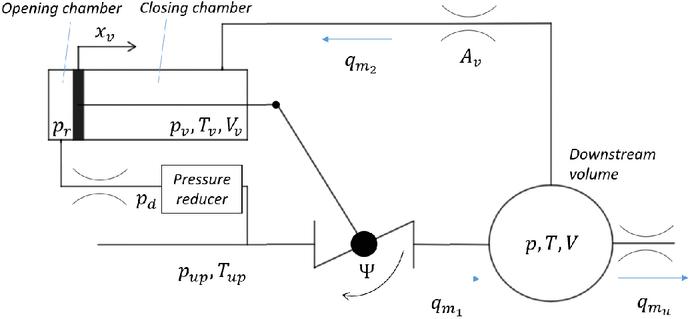
Figure 2 System schematic.
3 Case Study: Two-stage Valve
The pressure control valve under study is used to bring down the upstream pressure, , to a desired downstream pressure, . For a given reference pressure and a given return pressure , the valve regulates the opening of a butterfly valve through a piston-rod-crank system. The schematic of the valve is in Figure 2 whereas the Bond Graph representation of the valve is presented in Figure 3.
As shown in these figures, the reference pressure is guaranteed by a pressure reducer whereas the return pressure is provided by a feedback pipe connected to the downstream volume. The resulting force applied to the piston regulates the opening of the butterfly valve.
The mechanical modelling of the system regarding the piston movement is described by (10). The butterfly valve angle is written in terms of the piston position , from a kinematic analysis.
| (10) |
where is the equivalent mass of the moving parts, is the piston velocity, and are, respectively, the surface area of the piston at the opening and closing chambers, is the piston and butterfly valve combined friction, is the rod-crank kinematic factor and is the aerodynamical torque at the butterfly valve.
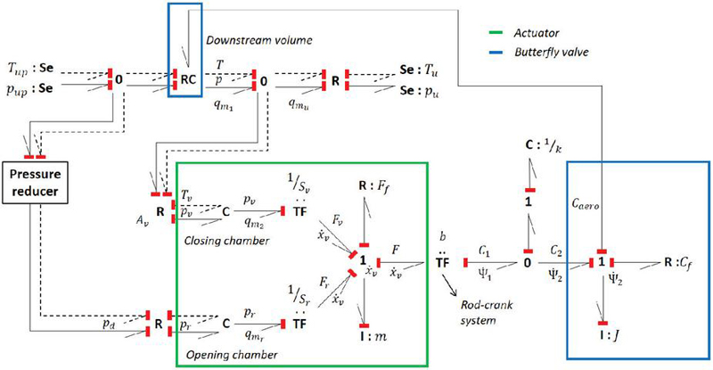
Figure 3 Bond Graph representation of the system.
Assuming a polytropic behavior (polytropic coefficient ) and negligible temperature variations in comparison to the average temperature in each volume, the dynamical behavior of the pressure in the downstream volume is represented by (11), while the dynamical behavior of the pressure in the closing chamber is represented by (12).
| (11) | |
| (12) |
where are the mass flow rates flowing to or from the downstream chamber as defined in Figure 2. The general mass flow rate through an orifice, according to ISO 6358-1 [12], is given by (13):
| (13) |
in which the pneumatic element is characterized by its sonic conductance, , and a critical pressure ratio, . This approximation is valid when the kinetic energy of the upstream flow is considered negligible. In this equation, is the mass flow rate, the upstream pressure, the downstream pressure, the upstream flow temperature, and and the air density and temperature at standard reference atmosphere. The flow coefficient, , is determined by (14) according to the flow regime delimited by the critical pressure ratio .
| (14) |
In order to reduce the model complexity and make the proposed approach clear enough without loss of generality, some additional hypotheses are then considered:
1. The pressure reducer guarantees a constant pressure in a way that the pressure inside the opening chamber is constant and equal to the reference pressure ;
2. The return conduit dynamics is fast enough to be modelled as an equivalent restriction, characterized by its area ;
3. The dry friction from the butterfly valve and the piston is not considered, and the viscous friction of both components is gathered in a single term where is the viscous friction coefficient assumed to be constant;
4. The aerodynamic torque is not considered;
5. The return flow is minor in comparison to the main flows and and can be neglected in the dynamical equation (11) of the downstream pressure.
Let us note that the dry friction term has naturally an influence on the system behavior, but by neglecting it in our method, it leads only to a more constrained solution for the design. Regarding the aerodynamic torque on the butterfly valve, its dependency on the flow through the valve and the butterfly angle [13] can be considered with the same approach if more precise results are required.
From these assumptions the model of the valve can be reduced to a fourth order system, considering as state variables the piston position , the piston velocity , the downstream pressure and the closing chamber pressure . The nonlinear model is formulated as (15):
| (15) |
with the pressures and the temperatures as inputs.
The dynamic behavior of the simplified model was compared to that of a detailed model developed using the Simcenter Amesim™simulation software (Figure 4) in order to verify that it properly represents the real system behavior.
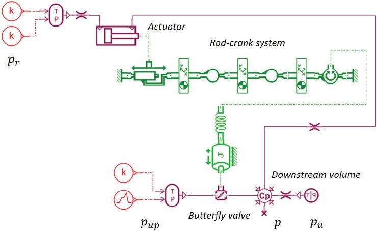
Figure 4 Simcenter AMESim™model of the valve.
4 Application
In order to study the system’s stability according to the design parameter, the first step is the linearization of the non-linear model (15) for small variations around the equilibrium point for given inputs values:
| (16) |
For given inputs and considering , the equilibrium point is defined by (17).
| (17) |
Once the matrix is formulated, the elements of the matrix that linearly depend on the analyzed parameters are separated from the other elements of the matrix as in (3).
The proposed method can be applied considering different forms of the Lyapunov function. In our case, a certain level of conservatism was added to the computational method such as a quadratic function form for the Lyapunov function and a certain type of dynamic behavior. Let us now discuss the conservatism degree related to the matrix .
One possibility is to consider that the Lyapunov function is built from a matrix constant and independent of the parameters . Another option, less conservative, would be to consider that the matrix is a function of as in (18):
| (18) |
where is the constant part of the matrix whereas the matrices are the terms of that depends on . In this case, one or more degrees of freedom are added to the optimization problem (6) and (9).
In this paper, two parameters are analyzed using this method: the viscous friction coefficient , and the flow area of the return orifice , defined by its diameter . Since the linearized state matrix obtained from (15) is linearly dependent of both parameters, from (3), the corresponding matrices can be expressed by (19), (20) and (21).
| (19) | |
| (20) | |
| (21) |
where is the reference value of the viscous friction and is the reference value of the orifice flow area.
5 Results
In order to determine the widest range of the parameter values in which the system is stable, an exhaustive study could consist in determining the eigenvalues of the matrix according to the parameter values. This step is not required in the proposed approach but it gives a reference (column 3 in Table 1) for the results that will be obtained from the proposed approach.
In the following, our approach is split into two sections. Section 5.1 deals with the stability analysis only, by determining the largest parameter range for which a Lyapunov function can be found to guarantee the stability constraint. Section 5.2 aims at defining more precisely the design parameter range, which satisfies stability and an additional constraint on the dynamical behavior, that is a minimum decay rate or a maximum damping parameter .
The study was implemented for each parameter at a time, it means that if is studied, is considered equal to its reference value and vice versa.
5.1 Stability Analysis
In this first case, an iterative procedure is used to determine a valid range for the studied parameter. From an initial value for , each iteration tries to find a Lyapunov function for the proposed parameter range. If no Lyapunov function is found, is reduced. Furthermore, if no function is found for any value of in this range, the parameter variation range is reduced and the procedure is restarted.
In this first example, the aim is to determine the admissible range of the viscous friction coefficient. The results are presented for sonic and subsonic flows in the butterfly valve and the minimum is afterwards deduced (Table 1).
Table 1 Stability analysis results without constraints on and
| Flow | From | |||||
| Condition | Eigenvalues | w/o Dependence | w/ Dependence | |||
| Parameters | on | Analysis | in () | in () | ||
| [N.s/m] | [N.s/m] | [] | [N.s/m] | [] | ||
| 21.25cm [N.s/m] | Sonic | |||||
| Subsonic | ||||||
Table 1 shows that the second formulation of the Lyapunov function, in which the parameter dependency is taken into account (column 5), enables to find a minimum value for the parameter that is smaller than the one obtain with a formulation with a constant matrix (column 4). The admissible parameter range is very close to the results obtained directly from the exhaustive eigenvalues analysis (column 3). This result is reasonable since the Lyapunov function with a polynomial form according to the parameter is less conservative, i.e., it offers additional degree of freedom compared to the simplest formulation with .
5.2 Using Design Specifications
Let us now impose a minimum or a maximum to determine the and minimum values that guarantee the desired dynamical behavior. In this case, the same kind of iterative procedure is used. Starting with the initial parameter range obtained from the eigenvalues analysis (column 3 in Table 2), the parameter range is iteratively reduced until a Lyapunov function that guarantees the desired value of or , is found.
Table 2 Minimum values of and for the imposed dynamic requirements on or
| Flow | From | |||
| Condition | Eigenvalues | |||
| Parameters | on | Analysis | w/o Dependence in : | |
| 21.5cm [N.s/m] | Sonic | |||
| Subsonic | ||||
| 21.5cm [mm] | Sonic | |||
| Subsonic | ||||
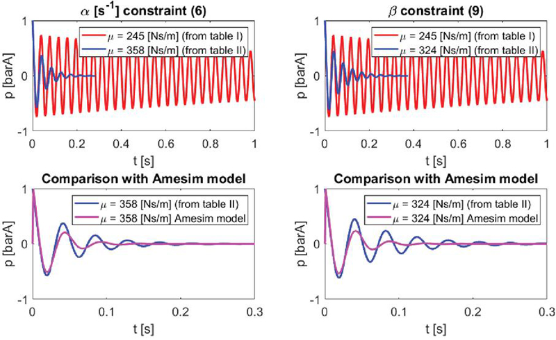
Figure 5 Downstream pressure responses (subsonic conditions) for the different minimum values of obtained according to the imposed constraint, and comparison between the analytical and simulation models.
As expected since the dynamical constraints are more severe, the admissible range for each parameter (column 4 in Table 2) is reduced in comparison with the initial range (column 3). Figure 5 shows the dynamic response of the pressure in the downstream volume when excited by a pulse in the subsonic case according to the minimum value of the viscous friction coefficient determined in each case and compared to the initial one.
As it can be observed (Figure 5), the dynamic behavior satisfies the specified constraint imposed by or . By considering both and , we can determine design rules that guarantee a much faster and less oscillatory response for the system. Figure 5 also shows a comparison of the pressure response obtained with the analytical model and the simulation model. It can be noticed that the dynamic behaviors of both models are very close for a given value of .
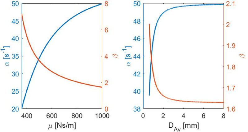
Figure 6 Evolution of and in parameter range in the subsonic case.
Once a Lyapunov function has been found for a parameter range, the asymptotic stability is proven and the minimum or maximum found is guaranteed for the whole parameter range. It is also possible to determine the variation of and in this parameter range by calculating the eigenvalues of the system. These results are shown in Figure 6 for the subsonic case.
This kind of results can illustrate how each physical parameter influences the dynamic response of the system. As it can be observed for the studied case, the dynamic response time gradually varies with the viscous friction coefficient, while the influence of the diameter of the orifice flow area stagnates passed a certain value.
6 Conclusion
This work proposed an LMI based analysis and design method that uses the decay rate and the damping parameter to find the physical parameters range that guarantees a desired dynamic behavior of a pressure regulation valve. The theory behind the method is firstly explained. An analytical nonlinear model of the two stage valve is then developed followed by its simplification and linearization. Then, the state matrix that depends on the physical parameters, is determined so the convex optimization approach can be implemented. The simulation results show that the method is capable of correlating physical parameters values to the dynamic response of the system with respect to a minimum decay rate and a maximum damping parameter .
Further work will aim at implementing the method for other physical parameters, for example, the dry friction and the length of the return pipe between the downstream volume and the closing chamber. This last case could require a order state space model. The approach can also be implemented to the whole air bleed system, taking into consideration the interactions between several valves and analyzing how physical parameters variations can influence the stability of the system as a whole. Experimental tests will also be planned to validate the approach and to verify the obtained design conditions.
References
[1] S. Boyd, L. El-Ghaoui, E. Feron and V. Balakrishnan, Linear Matrix Inequalities in System and Control Theory, Society for Industrial and Applied Mathematics, vol. 15, Philadelphia, 1994.
[2] M. Chilali, P. Gahinet and P. Apkarian, Robust pole placement in LMI regions, in IEEE Transactions on Automatic Control, vol. 44, no. 12, pp. 2257–2270, Dec. 1999.
[3] O. Ameur, P. Massioni, G. Scorletti, X. Brun and M. Smaoui, Lyapunov Stability Analysis of Switching Controllers in Presence of Sliding Modes and Parametric Uncertainties with Application to Pneumatic Systems, IEEE Transactions on Control Systems Technology, vol. 24, no. 6, pp. 1953–1964, Nov. 2016.
[4] T. Vaezi, M. Smaoui, P. Massioni, X. Brun, E. Bideaux, Nonlinear Force Tracking Control of Electrohydrostatic Actuators submitted to Motion Disturbances, 12th International Fluid Power Conference, Group F-2, pp. 221–230, 2020.
[5] A. Trofino and T. J. M. Dezuo, LMI stability conditions for uncertain rational nonlinear systems, International Journal of Robust and Nonlinear Control, vol. 24, pp. 3124–3169, 2014.
[6] D. Henrion and J. B. Lasserre, Convergence relaxations of polynomial matrix inequalities and static output feedback, IEEE Transactions on Automatic Control, vol. 51, Issue 2, pp. 192–202, February 2006.
[7] T. Dezuo, L. Rodrigues and A. Trofino, Stability Analysis of Piecewise Affine Systems with Sliding Modes, American Control Conference, pp. 2005–2010, Oregon, June 2014.
[8] R. Oliveira, P. Peres, Stability of polytopes of matrices via affine parameter dependent Lyapunov functions: Asymptotically exact LMI conditions, Elsevier Linear Algebra and its Applications, pp. 209–228, 2005.
[9] S. Prajna and A. Papachristodoulou, Analysis of Switched and Hybrid Systems – Beyond Piecewise Quadratic Methods, IEEE Proceedings of the American Control Conference, pp. 2779–2784, Colorado, June 2003.
[10] Mosek optimization toolbox for MATLAB – Version 9.3 https:/docs.mosek.com/9.3/intro.pdf.
[11] D. Karnopp, R. C. Rosenberg, System Dynamics: A Unified Approach, John Wiley & Sons, 1975.
[12] ISO 6358-1, Determination of flow-rate characteristics of components using compressible fluids – Part 1: General rules and test methods for steady-state flow, International Standard. Pneumatic fluid power, 2013.
[13] B. W. Andersen, The Analysis and Design of Pneumatic Systems, John Wiley & Sons, 1967
Biographies

Gabriel de Carvalho is currently pursuing his Ph.D. at the Ampère Lab (University of Lyon) at INSA Lyon, in collaboration with Liebherr Aerospace Toulouse. He obtained his Master’s degree in Mechanical Engineering from Clermont INP, France, in 2017, and he concluded his bachelor’s degree in Mechanical Engineering from UFRJ, Brazil, in 2020, through a double degree program facilitated by the CAPES/BRAFITEC exchange program. His research focuses on the stability and performance analysis of aircraft Air Bleed valves within the field of Control Engineering.

Paolo Massioni got his M.Sc. in Aerospace Engineering from Politecnico di Milano, Italy, in 2005, and his Ph.D. in Control Engineering from Delft University of Technology, The Netherlands, in 2010. From 2010 to 2012, he has been a postdoctoral researcher jointly at the University of Paris 13 and at the National French Aerospace Lab (ONERA), both in France. From the year 2012, he is a permanent academic staff member of the Laboratoire Ampère, at the French National Institute for Applied Science (INSA) of Lyon, France. His main research interests are distributed control, nonlinear systems performance and control of aerospace systems.

Eric Bideaux got his M.Sc. in Mechanical Engineering from Ecole Centrale de Nantes (France) in 1991, and a Ph.D. in Automation and Control from the University of Franche-Comté (France) in 1995 before joining the National Institute of Applied Sciences in Lyon (France). Since 2006 he is professor at the Ampère Lab (University of Lyon). His research fields are control engineering applied to mechatronic and Fluid Power systems with a focus on Bond Graph formalism for modelling, simulation and design of energy efficient systems.

Sylvie Sesmat received the Ph.D. degree from INSA Lyon Scientific and Technical University, Villeurbanne, France, in 1996. She is currently a Research Engineer with the Laboratoire Ampère, Villeurbanne. Her research interests include modelling and characterization of fluid power systems. Since 2007, she is involved in the international standardization in particular for standards concerning static and dynamic characterization of pneumatic components.

Frédéric Bristiel received a Mechanical Engineering degree from ENSAM in 2000 and has worked at Liebherr Aerospace Toulouse for 17 years in the valve design department. He took up the position of expert in 2015 and has been working on various French and European research projects, including the study of stability and performance analysis of aircraft Air Bleed valves in collaboration with the Ampère Lab (University of Lyon).
International Journal of Fluid Power, Vol. 25_2, 145–162.
doi: 10.13052/ijfp1439-9776.2522
© 2024 River Publishers