Load Handling Performance Comparison Between a Digital and a Conventional Hydraulic Winch Drive
Thomas Farsakoglou1,*, Perry Li2, Henrik C. Pedersen1, Morten K. Ebbesen3 and Torben O. Andersen1
1Mechatronics, Department of Energy, Aalborg University, 9220 Aalborg, Denmark
2Department of Mechanical Engineering, University of Minnesota, MN 55455 Minneapolis, USA
3Faculty of Engineering and Science, University of Agder, 4879 Grimstad, Norway
E-mail: thfa@energy.aau.dk; Lixxxo099@umn.edu; hcp@energy.aau.dk; morten.k.ebbesen@uia.no; toa@energy.aau.dk
*Corresponding Author
Received 09 October 2024; Accepted 12 August 2025
Abstract
Offshore winches commonly use conventional hydraulic drives, which are characterized by low energy efficiency. Digital displacement motors have shown promise for improving the energy efficiency of winch drive applications as they utilize digital valves for their operation. This paper compares the performance of a novel digital hydraulic winch drive and a conventional hydraulic winch drive with respect to their ability to control the load position of a commercial offshore knuckle-boom crane accurately. The considered digital winch drive consists of a digital displacement motor that operates in parallel with an electric motor. The power rating of the electric motor is small compared to that of the hydraulic motor, and its role is to smooth out the torque output of the digital displacement motor. The analysis shows that a smoother torque output reduces valve switchings and, therefore, increases the digital displacement motor’s volumetric efficiency. The drives’ performance is evaluated via simulations in four scenarios with varying conditions. The digital drive exhibits enhanced accuracy, achieving up to a 24 mm reduction in maximum load position error in three test scenarios, and performs comparably to the conventional drive in the fourth. Notably, the digital system controls the load with greater smoothness and fewer oscillations. These findings suggest that a digital displacement motor operating together with an electric motor presents a promising alternative for offshore winch drive applications.
Keywords: Digital hydraulics, winch drive, offshore, energy efficiency, valves.
1 Introduction
Winch drives are widely used by the offshore industry to control crane loads in subsea applications related to gas and oil but also for the offshore wind industry. In recent years, there has been an increasing interest in improving the energy efficiency of offshore winch drives in an effort to meet modern environmental criteria. An example of an offshore crane that utilizes a winch drive system for its operation is shown in Figure 1. The illustrated crane is rated for lifts up to , and it is produced by NOV, a globally acknowledged manufacturer of equipment for offshore applications [30].
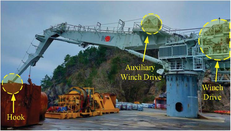
Figure 1 Offshore knuckle-boom crane from NOV placed on land. It is rated for loads up to 150 tons. Also shown in [6].
Traditionally, offshore winch drives have predominantly been hydraulic, which are known for their relatively low energy efficiency. In response to the growing imperative for sustainable operations, the offshore industry has been progressively pivoting toward the development of electric winch drives, especially for small scale drives. However, hydraulic systems offer certain benefits that would be challenging to replicate with electric drives [5]. Hydraulic motors have a significantly higher power to volume output ratio compared to electric motors. This characteristic allows hydraulic drives to be more compact, thus reducing the drive’s footprint on the limited and costly deck space. Furthermore, hydraulic motors excel in their ability to sustain intermittent, discontinuous, or extended high-torque demands without degradation in performance. Therefore, there is an interest within the industry to develop hydraulic winch drive systems that can rival the energy efficiency of their electric counterparts.
Digital Displacement Motors (DDMs) represent a promising advancement in hydraulic technology by offering scalability and increased energy efficiency compared to conventional hydraulic systems [5]. Unlike traditional variable displacement hydraulic motors, which continuously adjust their displacement to control power output, DDMs utilize digital valve pairs to control each chamber individually. By precisely managing each valve’s actuation, DDMs can achieve a high degree of control and efficiency, especially in part load operation, where the energy loss is much lower than for conventional drives. Several publications provide a thorough overview of the digital displacement technology, outlining its potential and development history [3, 10, 32, 34, 35]. Numerous studies and real-world applications have also demonstrated their superior energy efficiency in applications [13] such as off-road vehicles [8, 9, 14, 16], suspension systems [38, 40], and wave energy converters [1, 31]. However, there is limited research on utilizing DDMs for offshore winch drive applications.
Larsen et al. [15] showed experimental results that considered a winch driven by DDMs. However, they only considered a unique control method suitable for very low speeds, which was referred to as creep mode. The method controlled the pistons in a manner that allowed the shaft to move from one moment of equilibrium to the next. This allowed the motor shaft to move in a step-wise fashion, with each step corresponding to approximately . The method was considered unsuitable for normal winch drive operation, which involves higher velocities. Nordås et al. [25, 26, 28, 29] have extensively studied the use of DDMs for offshore winch drive applications. In their earlier works [25, 26], they provided an initial comparison between a digital and a conventional hydraulic winch drive, focusing on closed-circuit, pump-controlled systems. Their findings highlighted the digital hydraulic drive’s superior performance regarding reduced load position error and increased energy efficiency. However, this research only considered constant gravitational torque on the load side. Expanding upon this, [28] proposed a PID-controller to control the DDM’s displacement. This research incorporated a more detailed load-side dynamic model, accounting for wave-induced disturbance, friction, and wire elasticity. The results showed that the digital winch drive maintained a position error below throughout the tests under the influence of a disturbance with a peak-to-peak amplitude of approximately 2 m. Later, the same authors [29] conducted a comparative analysis of various control strategies for digital hydraulic winch drives aimed at precise winch position control and minimization of load position errors. The considered control schemes included a PI controller with inverse dynamics feedforward compensation, a sliding mode controller, and an adaptive controller. While the sliding mode and adaptive controllers showcased the smallest position error, they penalized energy efficiency due to frequent valve switching. The studies by Nordås et al. provide useful insights into the performance of DDMs in offshore winch drive applications. However, the displacement control strategy that was utilized to control the DDM, presented in [27], relies on switching a piston’s valves simultaneously, which results in significant volumetric losses [7]. Secondly, the authors did not consider a commercial offshore winch drive for comparison.
This paper investigates whether a highly energy-efficient digital winch drive can achieve load control precision that is comparable to or superior to a conventional hydraulic winch drive by comparing their control precision across different operating scenarios. The considered commercial drive is the winch drive indicated in Figure 1 and it is modeled and controlled based on publications made by Moslått et al. with NOV [19] and information provided directly by NOV. The digital hydraulic winch drive’s design is based on the commercial winch drive and was developed over several publications by Farsakoglou et al. [4, 6, 7]. In [4], the authors presented a methodology for selecting the digital valve specifications that allow the DDM to operate with high volumetric efficiency. The displacement control scheme that allows the DDM to respond sufficiently fast for the chosen application was presented in [7]. The number of pistons that is required to limit the DDM’s oscillatory torque output and control the load with the desired accuracy was determined in [6]. For this study, an electric motor is added, which operates in parallel with the hydraulic DDM and further smooths out the drive’s torque output and increases the drive’s control accuracy. It is shown that the addition of the electric motor also reduces the number of times that the digital valves switch states, thus increasing the drive’s energy efficiency. It is noted that the electric motor can be small in size, as it is only used for control purposes. The idea of using hydraulic actuation to transmit the majority of power and electric actuation for modulation was also exploited in the Hybrid Hydraulic-Electric Architecture (HHEA) [17]. Simulation results from four different considered cases demonstrate that the digital winch drive’s precision in load control matches and often surpasses that of traditional hydraulics. Thus, the results show that a digital hydraulic winch drive can offer superior load handling while drastically increasing energy efficiency whether the electric motor is included or not. Moreover, the proposed DDM can control the winch without the need for a gearbox, which is considered an unreliable component and is often the source of system failures. The addition of an electric motor further increases energy efficiency by reducing the number of required valve switchings.
This paper is organized as follows: Section 2 describes the mathematical models for simulating the dynamics of the load side, the conventional hydraulic drive, and the digital hydraulic winch drive. Section 3 introduces the digital displacement control strategies that are employed to regulate the displacement of the DDM. To reduce simulation time, Section 4 proposes a simplified model of the DDM’s torque output. The utilized control schemes for both the conventional and digital hydraulic winch drives are presented in Section 5. Further, Section 6 describes the different testing conditions that are used to compare the performance of the two drives. The results of the simulations are shown and compared in Section 7. Thereafter, Section 8 discusses the benefits and limitations of the digital hydraulic winch drive. Finally, the study’s conclusions are summarized in Section 9. A list of the abbreviations that were used in this paper is found at the end of the article.
2 Simulation Models
The following subsections describe and present the models that were used to model the commercial winch drive, digital winch drive, winch drum dynamics, and the effects of the offshore environment on the system.
2.1 Load Side Dynamics
The load side model considers the dynamics of the winch drum with the load underwater while the crane is under the influence of heave motion. The equations that are presented here are defined based on Figure 2 while the parameters are given in Table 1. The sea waves cause the ship to oscillate, which in turn causes the crane’s tip to oscillate relative to the seabed. However, due to the crane’s dynamics, the ship’s movement and the crane tip’s movement are not identical. The vertical oscillation of the crane’s tip, , is compensated by the winch drive. However, as this paper does not consider the dynamics of the crane, it is assumed that the winch is placed at the tip of the crane and oscillates vertically. Furthermore, the model assumes that the main wire dynamics can be sufficiently captured by modeling the wire as two equal masses that are connected by a spring and damper system. The two wire masses are assumed to have a rigid connection to the winch drum and load, respectively. Finally, the load’s position, denoted as , is measured from a fixed point relative to the seabed, which corresponds to the crane’s tip position when not affected by heave motion.
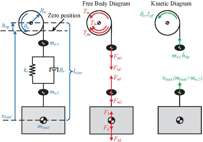
Figure 2 Load side dynamics (left), free body diagram (middle), and kinetic diagram (right).
Table 1 Load side dynamics parameters
| Parameter | Description | Value | Unit |
| Winch drum radius without wire | 1260 | mm | |
| Inertia of the winch drum without wire | 200 000 | kg m | |
| Young’s modulus of steel | 205 | GPa | |
| Wire’s cross section area | 3427 | mm | |
| Total wire length | 3000 | m | |
| Wire mass per meter | 26.9 | kg/m | |
| Gravitational acceleration | 9.81 | m/s2 | |
| Sea water density | 1025 | kg/m3 | |
| Steel density | 7850 | kg/m3 |
The winch drum angular acceleration and the load’s linear acceleration are defined using Newton’s 2nd law yielding:
| (1) | ||
| (2) |
where denotes the effective drum radius, the wire force, , , and the gravitational force acting on the upper wire mass, the lower wire mass, and the load, respectively. denotes the effective drum inertia, the load buoyancy, and the load drag. The variables , , and denote the crane tip’s position, velocity, and acceleration due to the induced net heave motion and are further explained in Eq. 12–14.
As the winch drum rotates, it unwinds or retracts wire; therefore, the drum loses or gains mass depending on the direction of its rotation, resulting in a variable drum inertia. As the wire is wrapped around the drum in layers, as shown in Figure 3, the effective winch drum radius is also variable. However, each layer contains approximately of wire while the load moves at speeds up to . Thus, the drum radius is assumed to remain constant during the simulations. Therefore, the radius of the winch drum needs to be considered only during initialization to correspond to the appropriate wire layer depending on the amount of wire that has been released.
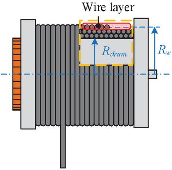
Figure 3 Winch drum’s wire layers illustration.
The wire’s elasticity is modeled by a single spring and damper system as suggested by DNV [2]. Thus, the mass of the released wire is divided into two equal parts:
| (3) |
where the upper mass is assumed to be rigidly attached to the drum, and rigidly attached to the load. Thus, the drum’s inertia is defined as:
| (4) |
where represents the drum inertia without the wire, including the inertia from the motor’s shaft and gears. The wire inertia that is wrapped around the drum is defined as:
| (5) |
where denotes the amount of released wire. The force produced by the spring and damper dynamics can be defined as:
| (6) |
where denotes the drum’s angular velocity, the drum’s angular position, the load’s linear velocity, and the load’s position. The wire’s stiffness is given as:
| (7) |
The damping coefficient is defined from [39]:
| (8) |
where the damping ratio is chosen for an underdumped system [22]. The seawater effects on the load can be identified by a buoyancy force and a drag force as defined in [2].
| (9) | ||
| (10) |
where is the load’s volume, and the load’s shadow area. The considered load is assumed to consist mostly of steel parts with some cavities that fill up with seawater when submerged. Therefore, the load density is defined as:
| (11) |
The load is assumed to have a rectangular box shape, with a fixed height of , while the load’s shadow area varies depending on the load’s mass.
When operating offshore, the crane’s tip oscillates vertically due to the ship’s movement. This oscillation is attributed to the ship’s heave, pitch, and roll motions, which are caused by sea waves. The net heave motion disrupts the ability of the operator to handle the load accurately with respect to another surface, such as the seabed. Accurate estimation of heave motion requires knowledge of the sea state, the ship’s response amplitude operators (RAO), and the structure of the crane. A sea’s state is typically sufficiently modeled with a JONSWAP wave spectrum; however, RAO and crane models can be difficult to obtain. For this study, previous analyses have shown that it is sufficient to approximate the heave motion on the crane’s tip as a sum of sine waves:
| (12) |
where the first sine wave has an amplitude of and a period of and for the second sine wave and . This method for modeling the heave motion results in a repetitive heave motion; however, this does not influence the results of this study as analyses have shown that this method sufficiently captures the main dynamics of heave motion that are produced from a JONSWAP spectrum. The crane’s tip velocity and acceleration due to heave motion are given as:
| (13) | ||
| (14) |
Equations (12–14) are visualized for a time period of in Figure 4.
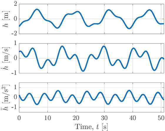
Figure 4 Crane’s tip heave motion dynamics over .
2.2 Conventional Drive
The conventional drive is divided into two subsystems: the active and the passive. These are indicated by dashed boxes in Figure 5. The control methodology for the drive is explained in Section 5. The subsystems operate in parallel, with the passive system maintaining a quasi-constant pressure and adjusting the motors’ displacement to produce a constant torque to negate the gravitational torque produced by the load. A double-piston accumulator is employed to enhance the passive subsystem’s capacity to sustain a nearly constant pressure drop across the motor. The active system is tasked with following the operator’s input while compensating for friction and the heave motion. The active system is pump-controlled, while the motor’s displacement is only altered when the winch drum’s radius changes [22]. Every motor is equipped with a gearbox that increases its torque output and reduces its speed. An additional torque increase is achieved via a pinion-to-ring gear connection, which connects the motor shafts to the winch drum.
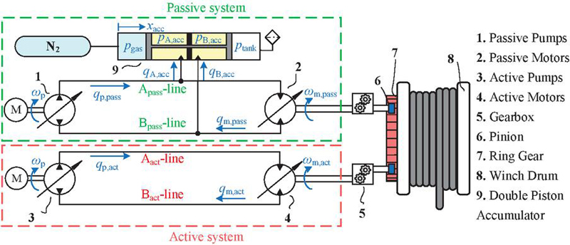
Figure 5 Conventional active/passive hydraulic winch drive schematic, inspired by [6].
The model for the conventional drive is defined based on the work of Moslått, who has published several experimental studies for the considered drive [21, 18, 22, 20] and developed a digital twin for a similar drive [23]. The parameters for the conventional drive are found in Table 2.
Table 2 Winch drum’s variables and parameters
| Parameter | Description | Value | Unit |
| Hydraulic drive specifications | |||
| Number of active motors | 3 | - | |
| Number of passive motors | 8 | - | |
| Max. displacement of motors | 215 | cm/rev | |
| Max. displacement of pumps | 855 | cm/rev | |
| Angular velocity of active pumps | 1800 | rpm | |
| Effective bulk modulus of oil | 8000 | bar | |
| Hydraulic line volume | 22 | l | |
| Total gear ratio | 479 | - | |
| Accumulator specifications | |||
| Maximum piston stroke | 2152 | mm | |
| Accumulator chamber dead volume | 18.9 | l | |
| Piston-side surface area | 2463 | cm | |
| Rod-side surface area | 1756 | cm | |
| Gas charge pressure | 207 | bar | |
| Gas volume | 4675 | l | |
| Piston’s mass | 1387 | kg | |
| Piston’s viscous friction | 10 | Ns/m | |
| Accumulator orifice flow coefficient | 1274 | l/min/ | |
The pressure dynamics of the active and passive subsystems are given as,
| (15) | ||
| (16) | ||
| (17) | ||
| (18) |
where and are the pressure drops from the A-line to the B-line for the active and passive systems, respectively. The flow from the motors and pumps is given in a general form by Equation (19),
| (19) |
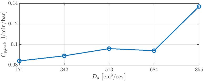
Figure 6 Lookup table for pump leakage conductance with respect to the pump’s displacement.
where is the number of motors/pumps, the angular velocity, the displacement, and the normalised swash plate displacement. The subscript may represent either pumps or motors for the active and passive subsystems, e.g., when considering the pumps of the passive system, then the subscript . The response of the motor/pump swash plate is modeled as a second-order transfer function:
| (20) |
For the pumps the natural frequency is determined to and the damping ratio . For the motors the natural frequency is determined to and the damping ratio . The values for the damping coefficients and natural frequencies are defined based on the work of Moslått et al. [22].
The leakage conductance in each subsystem is defined as the sum of the motors’ and pumps’ conductance along with a conductance that represents the unidentified leakages in the system. The system leakage was determined via an analysis that verified the conventional drive model based on experimental data from the drive operating without load. However, the analysis is not presented in this paper due to the fact that it contains confidential data.
| (21) |
The pump leakage conductance is given by linear lookup tables as a function of the pump’s displacement as illustrated in Figure 6. The values for the lookup tables are based on experiments presented by Moslått et al. [19] while was set to .
Experiments by Moslått et al. [19] have shown that the motor’s leakage coefficient can be sufficiently represented as a function of the motor’s speed, as shown in Equation (22):
| (22) |
where m3/Pa and m3/s/Pa. The accumulator’s piston movement is modeled using Newton’s 2nd law as shown in Equation (23). The accumulator’s piston position, velocity, and acceleration are denoted as , , and , respectively.
| (23) |
while the pressure dynamics of the double-piston accumulator are defined with the continuity equation:
| (24) | ||
| (25) | ||
| (26) |
The gas pressure dynamics are assumed to be adiabatic; therefore, the polytropic index 1.4. Any force contribution from the tank pressure is also neglected. The flows to the accumulator chambers pass through cartridge valves and are thus modeled by the orifice equations:
| (27) | ||
| (28) |
The torque contribution from the motors is given as:
| (29) | ||
| (30) | ||
| (31) |
The motor torque losses are modeled based on the findings of Moslått et al. [21]. The value of corresponds to either the active or passive system.
| (32) | |
| (33) |
The parameters for Equation (33) are listed in Table 3. The remaining friction in the system is modeled with a single function [21].
| (34) |
The parameters for Equation (34) are listed in Table 4.
Table 3 Parameters for A6VM215 motor friction
| Parameter | Value | Unit |
| Nm s | ||
| Nm s/m | ||
| – | ||
| Nm | ||
| m/N |
Table 4 Parameters for system friction
| Parameter | Value | Unit |
| 328 10 | – | |
| 0 | Nm | |
| 3.15 | Nm | |
| 0.06 | rad/s | |
| 0.00851 | Nm s | |
| 121 10 | – |
2.3 Digital Hydraulic Drive
The topology that is considered for the digital hydraulic winch drive consists of a large DDM with 77,000 cm3/rev operating in parallel with an electric motor, as shown in Figure 7a. Compared to the conventional drive, the DDM is not equipped with gearboxes but connects with the winch drum solely via a pinion-to-ring gear connection. Additionally, the pressure on the high-pressure line and low-pressure line is maintained approximately constant, and the load is controlled by adjusting the motor’s displacement. The electric motor is equipped with a gearbox that increases its torque output and reduces its velocity, which in turn connects to the ring gear. The electric motor is not necessary for the digital winch drive’s operation. However, DDMs are known for their oscillating torque output, which can impede the drive’s performance. Therefore, the role of the electric motor is to aid to reduce the DDM’s torque oscillations and allow the drive to achieve a smoother torque output. The benefits of utilizing an electric motor in parallel with the DDM are further elaborated in the simulation results in Section 7.
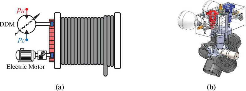
Figure 7 Digital Winch Drive System. (a) A simplified representation of the proposed offshore digital winch drive. (b) 3D model showcasing a five-piston radial piston motor, with one chamber controlled by a pair of digital valves.
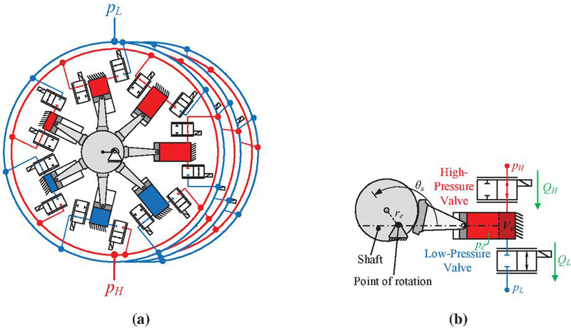
Figure 8 Sketches of a DDM inspired by [7]. (a) Basic depiction of a digital displacement motor featuring three modules, each consisting of seven pistons. (b) Sketch of an individual piston from the digital displacement motor under consideration.
The considered DDM consists of 39 pistons, which are organized into three modules with thirteen pistons each and share a common shaft. For illustrative purposes, a DDM with 21 pistons, organized in three modules with seven pistons each, is shown in Figure 8a. The pistons are distributed equally around the shaft for each module and for the motor as a whole. A previous study has shown that 37 pistons are sufficient [6]. However, due to physical limitations, the number has been increased to allow for a feasible piston distribution. The flow to the cylinders is independently controlled by a pair of digital valves that connect the piston’s chamber to the high- and low-pressure lines, as shown in Figure 8b. The parameters for the equations that are presented in this section are defined in Table 6. The shaft speed is denoted by , while the shaft angle introduces a relative phase shift for each piston:
| (35) |
The pressure dynamics of each chamber are governed by the high-pressure valve flow , low-pressure valve flow , and the piston’s volumetric flow rate :
| (36) | ||
| (37) | ||
| (38) |
where and indicate the normalized spool position of the High-Pressure Valve (HPV) and Low-Pressure Valve (LPV), respectively. The cylinder’s volume , volumetric flow rate, and shaft torque are given as:
| (39) |
Thus, the total torque output for the DMM , after considering the pinion to ring gear connection, is given by Equation (40) while the torsional losses are defined by Equation (41).
| (40) |
The motor torque losses for the DDM are unknown. Therefore, the friction model is simplified and adjusted to fit that of the conventional motors.
| (41) |
Table 5 Parameters for DDM friction
| Parameter | Value | Unit |
| 1430 | Nm s | |
| 1.1 10 | m/N |
Table 6 Parameters for the digital displacement motors, digital valves, and winch drive
| Digital Winch Drive Parameters | |||
| Symbol | Description | Value | Unit |
| pinion to ring gear ratio | 14.17 | – | |
| Max. operating motor velocity | 74 | rpm | |
| Min. operating motor velocity | 2 | rpm | |
| DDM Parameters | |||
| Symbol | Description | Value | Unit |
| Number of pistons | 39 | – | |
| Shaft’s eccentric radius | 50 | mm | |
| Piston’s cross sectional area | 198 | cm2 | |
| Effective oil bulk modulus | 15 000 | bar | |
| High pressure | 330 | bar | |
| Low pressure | 25 | bar | |
| Piston dead volume | 99 | cm | |
| Piston displacement volume | 1977 | cm | |
| Digital Valve Parameters | |||
| Switching time | 25 | ms | |
| Flow coefficient | 2900 | min | |
The parameters for Equation (41) are found in Table 5. The remaining friction in the system is assumed negligible compared to the motor friction and is disregarded. The valve’s spool motion is modeled using a sigmoid function. As a valve closes, it experiences a constant negative acceleration in the initial half of its switching time and a constant positive acceleration in the subsequent half, as detailed in Eq. (42). The signs within the piecewise function reverse when the valve is opening. This modeling technique has been utilized in diverse studies [37, 33]. It is noted that this method for modeling the valve’s spool assumes that the initial conditions are zero and that the valve switch occurs at time .
| (42) | ||
| (43) |
In this context, represents the normalized position of the valve spool, and indicates the acceleration of the spool. The torque output of the electric motor on the winch drum is modeled as a first-order transfer function scaled by the total gear ratio. This model for the electric motor has also been used for applications considering fully electric winch drives as in [11].
| (44) |
where the gain is chosen to correspond to the maximum torque output of one of the conventional motors, which is equal to one-tenth of the DDM’s maximum torque output. The time constant is , thus the electric motor’s settling time is based on the criterion for first-order systems. The variable is the motor’s input, which is regulated by a controller as defined in Section 5. By considering that the winch drum’s maximum speed is approximately , the electric motor’s maximum power output can be conservatively calculated:
| (45) |
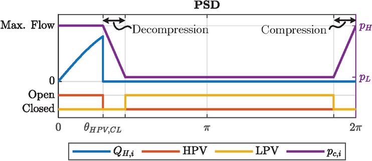
Figure 9 Valve timing for a single piston over a revolution with PSD strategy.
3 Digital Displacement Strategies
The displacement control strategies that are considered for this study are Partial-Stroke Displacement (PSD) and low-speed Partial-stroke Sequential Displacement (ls-SPD) strategies, illustrated in Figure 9 and Figure 10, respectively. The figures consider a single piston during a full revolution. A PSD strategy adjusts the motor’s displacement by varying the closing angle of the HPV which is denoted as . The opening of the HPV commences when the shaft angle is zero, corresponding to the piston’s top dead center. It is noted that the opening of the HPV could also be chosen at different angles; however, opening the HPV at the top dead center yields minimal losses, and therefore, it is widely preferred. The motor’s displacement can be given as a function of a normalized displacement input , as:
| (46) | ||
| (47) |
The LPV is closed prior to the HPV opening in order to allow the chamber to pressurize. Similarly, the LPV is opened after the HPV has closed to depressurize the chamber. Since valve actuation is angle-dependent, at low shaft speeds the displacement’s update rate can be very slow and compromise the motor’s performance. For example, at , each piston could update the opening/closing valve angles every . Therefore, at low speeds, the ls-SPD strategy is utilized.
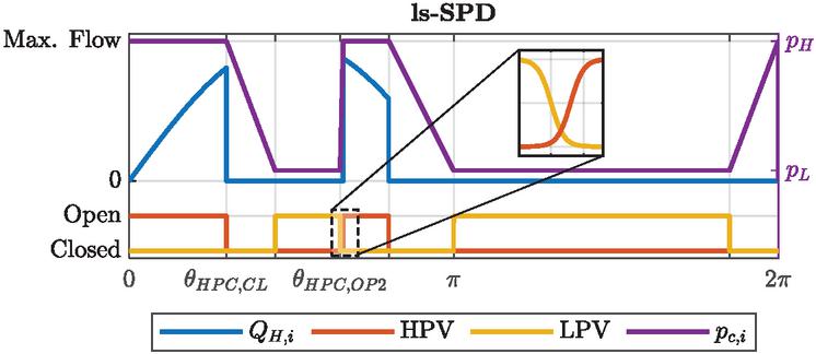
Figure 10 Valve timing for a single piston DDM over a revolution with ls-SPD strategy.
The ls-SPD strategy was first introduced by Farsakoglou et al. [7] to increase the displacement response time of DDMs at low speeds. The method resembles a PSD strategy; however, the ls-SPD allows the HPV to reopen multiple times during a cycle, as shown in Figure 10. In the example shown in the figure, the HPV is closed at based on the value of . At a later time, the value of has increased, and therefore, the HPV is reopened at . Any reopening of the HPV occurs without any precompression, thereby increasing losses compared to the PSD strategy. However, the results of Farsakoglou et al. showed that when the valve’s size and switching time have been chosen appropriately, the motor retains high volumetric efficiency.
The reopening of the HPV occurs with a small overlap with the closing of the LPV, thus resulting in both valves being simultaneously partially open for of their total switching time. This method allows for the chamber to be pressurized via the HPV while preventing the piston’s movement from depressurizing the chamber, as that could create cavitation. The time period that both valves remain partially open is referred to as a valve timing overlap. The chosen valve timing overlap value highly depends on the application. Generally, larger values ensure that cavitation is avoided but decrease the volumetric efficiency of the motor as larger amounts of oil flow directly from the high- to the low-pressure line. For this study, the overlap value is set at based on the previous findings of Farsakoglou et al. [7], as it is the same digital hydraulic drive.
4 Simplified DDM Model
The high number of cylinders and the frequent switchings that the ls-SPD introduces result in a stiff system that significantly slows down the simulation. Therefore, a simplified method for modeling the DDM’s torque output is utilized, which sufficiently captures the torque dynamics. The considered method discards the pressure dynamics and considers the chamber pressure as a function of the HPV’s normalized spool position :
| (48) |
To illustrate that the proposed simplification approximates the motor’s dynamics, Figure 11 is used. The figure shows the DDM’s torque response using the aforementioned simplification and the one resulting from the model presented in Section 2.3. A sinusoidal displacement trajectory with an increasing frequency is given as input, shown at the top of the figure. The considered DDM consists of seven pistons and rotates with a constant shaft speed of . The torque output of the DDM with the simplified method is indicated with a dashed orange line, while the model that includes pressure dynamics is illustrated with a solid blue line. From the figure, it is observed that the simplified method closely tracks the output that is produced when considering pressure dynamics. As shown in the magnified part of the figure, the simplified model results in a more abrupt torque output as the chamber is instantaneously depressurized instead of being a function of the motor’s shaft speed as indicated by Equation (36).This result in the error spikes that are shown in the bottom of Figure 11. However, these spikes have a short time span which results in an RMS error of , which is below of the maximum torque and is deemed acceptable.
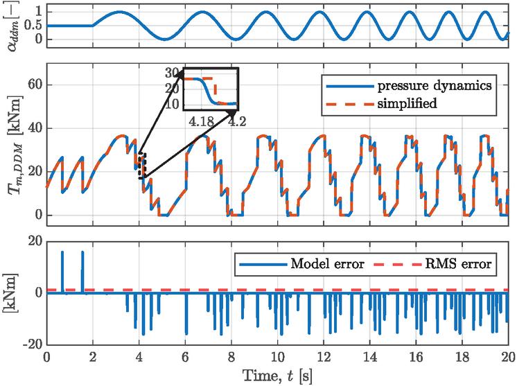
Figure 11 Comparison of DDM’s torque response with detailed pressure dynamics versus a simplified model.
5 Drive Control Schemes
This section describes the control schemes for the conventional and digital hydraulic winch drives.
5.1 Conventional Drive Control
The control for the conventional drive, illustrated in Figure 12, was designed based on the work of Moslått et al. [24]. The passive drive utilizes two PI controllers to control the displacement of the pumps and motors in order to maintain constant pressure in the hydraulic lines and balance the load’s gravitational torque. The control gains for pressure control are Pa-1 and s/Pa while for the torque control N-1m-1 and s/Nm. Therefore, the torque controller’s break frequency corresponds to , while the pressure controller’s break frequency is . The break frequencies were chosen in this manner as the pressure dynamics are significantly faster than the equivalent load’s mass, which varies slowly. The active drive utilizes only a P gain and a feedforward term to control the active pumps’ displacement:
| (49) | ||
| (50) |
where the gains for the feedforward signal are s and s2 while for the P gain .
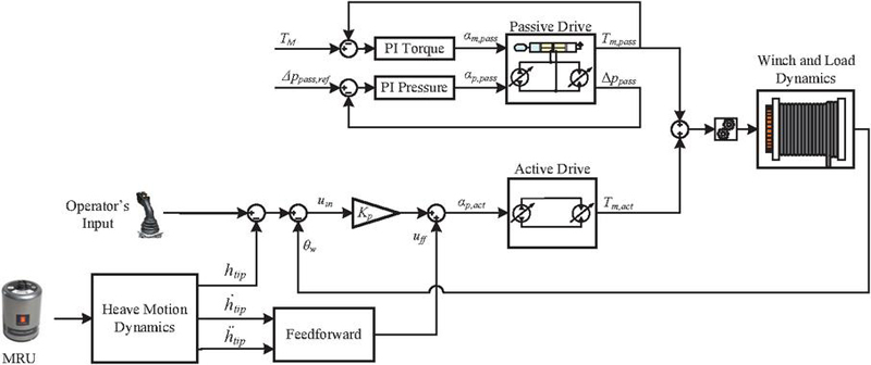
Figure 12 Control scheme for the conventional drive.
5.2 Digital Drive Control
The control scheme used by the digital hydraulic winch drive is illustrated in Figure 13. The digital hydraulic drive control signal is generated by a PID-controller and supplemented by a feedforward signal. The PID gains are tuned at m, ms, and s/m. The feedforward signal is calculated based on simplified inverse dynamics by only considering the desired motor output torque and the load’s gravitational torque:
| (51) |
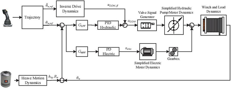
Figure 13 Control scheme for the digital drive.
The signal is then translated into digital signals for all the valves of the DDM as described in Section 3. When the motor’s shaft speed is above , then the PSD strategy is used, while below , the ls-SPD is utilized. The operating speed range for each strategy is designed based on the conclusions from Farsakoglou et al. [7]. The electric motor is regulated by a PD controller. The controller’s output, , is constrained within the range of –1 to 1. It features a proportional gain m and a high derivative gain s/m.
Both the electric motor and the DDM are controlled based on the load’s position error. However, the position error signal is filtered via Low-Pass Filter () and a High-Pass Filter () so that the DDM receives only the lower frequencies while the electric motor receives and compensates only the higher frequencies. The transfer functions for the filters are defined as:
| (52) |
which result in break frequencies of and for the low-pass filter and high-pass filter, respectively. Effectively, this means there is a bandpass area where both the electric motor and the DDM are active. While this may seem a bit counterintuitive, the different dynamics of the electric and hydraulic motors have yielded this to be the most optimal solution as some of the pressure ripples resulting from the switching of the valves are compensated through the electric motor, thus yielding lower overall torque ripples.
6 Considered Simulation Tests
To thoroughly assess the two drives across the crane’s entire operating range, four distinct tests have been designed which are summarized in Table 7. These tests involve the crane operating at both the maximum and minimum load capacities. As for the operating depth, the two considered cases correspond to depth values close to the crane’s maximum and minimum operating depths, which correspond to a wire with high and low stiffness.
Table 7 Test parameter summary
| Load [ton] | Load depth [m] | |
| Test A | 20 | 200 |
| Test B | 150 | 200 |
| Test C | 20 | 2950 |
| Test D | 150 | 2950 |
The considered operator’s input dynamics are shown in Figure 14 while the crane’s tip dynamics resulting from heave motion are shown in Figure 4. The operator’s input trajectory is designed based on information received from NOV. The trajectory is designed to contain the fastest and slowest speeds that the load is desired to move which corresponds to and . It should be noted that the wire speed, i.e. the linear speed resulting from the drum’s movement, can exceed the load’s maximum speed by orders of magnitude as it is equal to . The wire speed is required to reach such speeds in order to compensate for the heave motion.
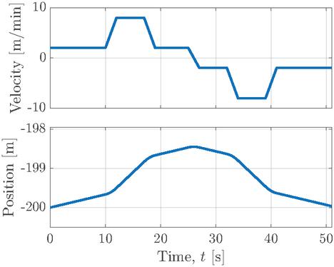
Figure 14 Considered load velocity and position trajectory.
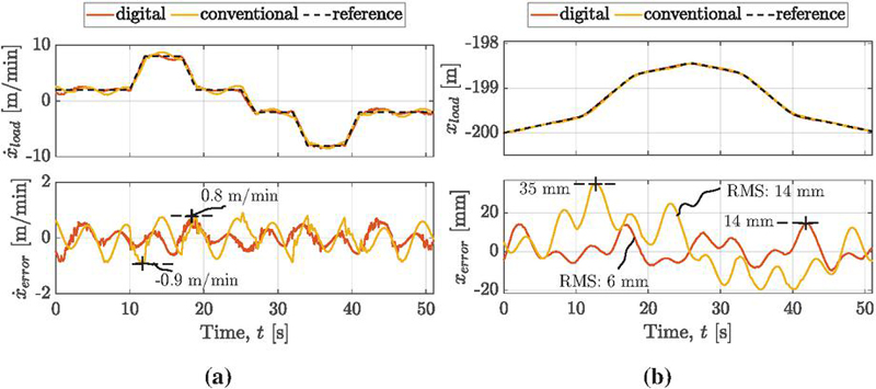
Figure 15 (a) Load velocity and velocity errors for Test A. (b) Load position and position errors for Test A.
7 Simulation Results
This section presents the simulation results that were obtained from the tests presented in Section 6.
7.1 Test A: small load, low depth
The resulting load velocity and position for Test A are shown in Figure 15a and Figure 15b, respectively. For this test, the digital winch drive shows superior performance, with the load’s largest position deviation from the reference being . For the conventional drive, it was . The Root Mean Square (RMS) error is also significantly lower, compared to for the conventional drive. Additionally, the conventional drive results in an oscillatory load movement characterized by larger amplitudes and longer periods than the load’s movement resulting from the digital drive. This load movement behavior stresses the system and complicates the operator’s ability to land the load safely. However, both drives are able to control the load accurately and maintain the load’s position error well below the offshore industry’s requirement of . To highlight the effect of the electric motor on the performance of the digital winch drive, Figure 16 is used. The figure shows the total torque output of the digital winch drive for test A along with the torques produced by the DDM and the electric motor . The magnified section illustrates that the fast dynamics of the electric motor allow the drive to significantly reduce the torque oscillations that are introduced by the DDM. However, as the DDM’s torque is reduced in a step-wise fashion when closing the HPV, the electric motor with the implemented controller requires approximately to respond to this abrupt change. This causes torque spikes to occur at the drive’s output with an amplitude of . These torque spikes can fatigue system components over a prolonged time period, such as the pinion to gear ring connection. However, the torque spikes may be reduced by including a feedforward signal to the electric motor’s control prior to closing an HPV. However, such a solution has not been considered for this work and is thereby proposed for future studies.
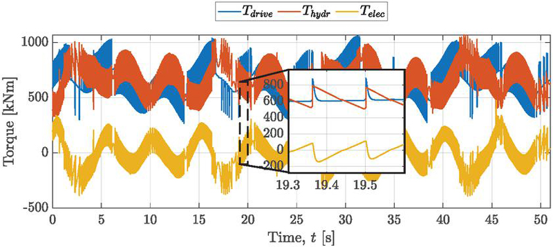
Figure 16 Resulting digital winch drive torque, DDM torque, and electric motor torque for test A.
To illustrate the benefits of utilizing an electric motor in parallel with the DDM Figure 17 is used. The figure shows the load’s velocity and position for test A while utilizing only the DDM, without retuning the controller. As seen from the figure, the drive’s performance has slightly deteriorated with the load’s position error peaking at with an RMS value of .
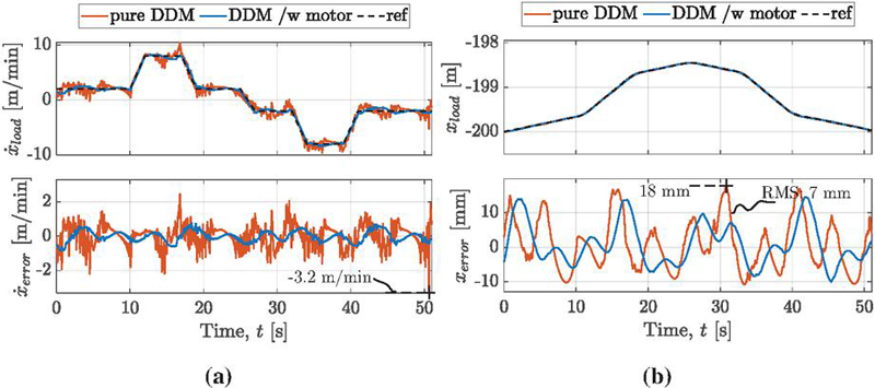
Figure 17 Digital winch drive performance without utilizing the electric motor compared to with the assistance of the electric motor.(a) Load velocity and velocity error for Test A. (b) Load position and position error for Test A.
Another benefit that is yielded by utilizing the electric motor is that the number of HPV switchings is drastically decreased. Without the electric motor to reduce the DDM’s torque oscillations, the HPVs are switched for a total of 1384 times. When the electric motor is used to smooth out the drive’s torque, the HPVs are switched 801 times. The number of times that the HPVs switch over a cycle can have a significant impact on the motor’s volumetric efficiency but also on the fatigue properties of the system. In the work presented by Farsakoglou et al. [7], it was shown that a volumetric efficiency near can be achieved with the ls-SPD strategy when the HPV is switched on twice over a revolution. However, if the HPV is opened multiple times over a revolution then a significant drop in the motor’s volumetric efficiency is observed. For example, in Figure 18 the HPV of a single cylinder is switched 12 times over a revolution while the shaft rotates at a speed of . By evaluating the cylinder’s efficiency with the method that was utilized by Farsakoglou et al. [7], it is observed that the cylinder’s volumetric efficiency drops down to . Therefore, as the addition of the electric motor reduces the total number of valve switchings, it results in the DDM operating with a higher volumetric efficiency. Additionally, a high number of valve switchings reduces the valve’s lifetime and increases maintenance costs.
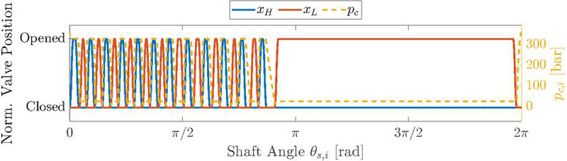
Figure 18 Multiple HPV switchings over a cycle for a single piston.
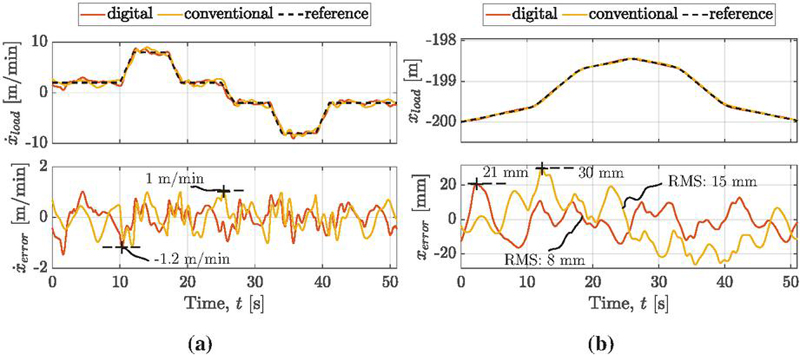
Figure 19 (a) Load velocity and velocity errors for Test B. (b) Load position and position errors for Test B.
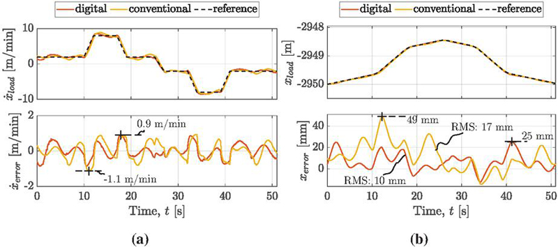
Figure 20 (a) Load velocity and velocity errors for Test C. (b) Load position and position errors for Test C.
7.2 Tests B, C, and D
The remaining tests are presented in Figures 20-21, and the results are summarized in Table 8. From the table, it is observed that the digital hydraulic drive achieves roughly half the position error of the conventional drive throughout tests A, B, and C. For test D, both drives achieve the same maximum load position error of . However, the digital winch drive yields a slightly lower RMS value of compared to for the conventional drive. However, both drives have an acceptable performance as the load position error remains well below the offshore industry’s requirement maximum acceptable value of . As was observed in test A, the digital drive’s behavior is characterized by high-frequency oscillations with small amplitude. In contrast, the conventional drive tends to result in lower frequency oscillations with a higher amplitude. The smoother load control of the digital drive may be attributed to its faster response due to the ls-SPD strategy. The faster response is further enabled by maintaining the line pressure constant, as secondary controlled hydraulic drives are known for offering a faster response since the hydraulic oil is always compressed. In a practical application, the drives’ performance is expected to change due to parameters that have not been considered during the simulations. Such parameters include slack in the pinion to ring gear connection, measurement errors, and slight deviations in the system models.
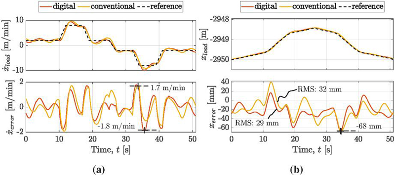
Figure 21 (a) Load velocity and velocity errors for Test D. (b) Resulting load position and position errors for Test D.
Table 8 Load position results for the considered tests
| Digital Winch Drive | Conventional Drive | |||
| max | RMS | max | RMS | |
| Test A | ||||
| Test B | ||||
| Test C | ||||
| Test D | ||||
8 Discussion
This section presents a discussion of the benefits and drawbacks of the proposed digital winch drive with respect to its operation and practical implementation.
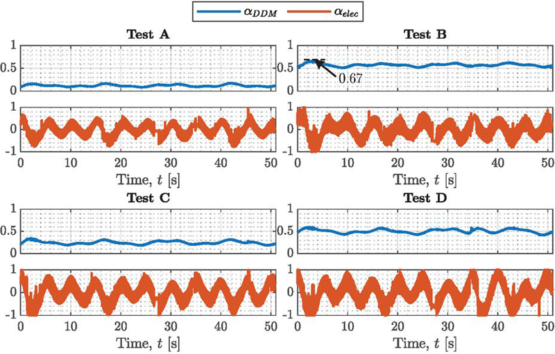
Figure 22 DDM and electric motor control signals for tests A to D.
Figure 22 shows the outputs of the PID and PD controllers for the DDM and electric motor, respectively, throughout all the tests. The largest value for is observed in test B and corresponds to 0.67. This indicates that the parameters that were chosen for the DDM were oversized. Therefore, a DDM with a smaller displacement could be used. Additionally, the PSD and ls-SPD strategies produce the largest oscillations the closer the DDM operates to displacement [27]. For tests B and D, operating a DDM with a smaller displacement or reduced supply pressure could allow for the resulting control signal to move closer to displacement, where the DDM shows the smoothest torque output and highest volumetric efficiency. For tests A and C, the displacement signal would move closer to displacement, which would result in larger torque oscillations. However, the DDM would operate more efficiently since its volumetric efficiency is reduced at low displacements. Another observation from Figure 22 is that the electric motor does not operate with its maximum torque for a prolonged period of time. In order to evaluate the power estimation Eq. (45) is utilized and, the power output of the electric motor throughout all tests is calculated. It is found that the highest power consumption occurs for test D and is shown with the blue line on the left plot in Figure 23. The plot on the right illustrates the DDM’s power output to illustrate the difference in power rating between the two motors. From the figure, it is seen that the highest power output of the motor is only reached at and is equal to . As the electric motor compensates for the DDM’s torque oscillations, choosing a DDM with a higher number of pistons can decrease the electric motor’s power output. In Figure 23, the power output of the electric motor when using a DDM with 133 pistons is shown with the orange line. It is seen that the maximum power output is reduced to . Therefore, when designing a digital hydraulic winch drive, the number of pistons could be optimized to determine the size of the electric motor. In this example, the chosen number of 133 pistons is unrealistic; therefore, a future investigation could consider how the digital winch drive would behave with a DDM utilizing 39 pistons and a electric motor. Including an electric motor to operate in parallel with a DDM can provide additional benefits. For example, the electric motor could be used to handle the winch when operating with an empty hook or smaller loads without the need to use the hydraulic system.
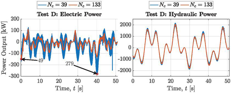
Figure 23 Power output of electric motor (left plot) and DDM (right plot) for test D for a DDM with 39 pistons and a DDM with 133 pistons.
Finally, despite the various potential benefits that a digital hydraulic winch can offer, it also imposes certain limitations. The digital valves require accurate feedback of the shaft’s angular position. However, the Programming Logic Controllers (PLCs) that are used in such applications typically have low computational power and might be unable to process the high-resolution signal that is required to measure the shaft’s angular position accurately. Furthermore, the digital valves that the DDM requires to yield high volumetric efficiency in the considered application are required to offer a high flow rate, low switching time, and be able to open against high pressure [4]. Such valves are produced by few suppliers and have a high cost. The overall cost can increase further when considering DDM designs with a higher number of cylinders, as a pair of valves is required for the control of each piston. Another parameter that has not been considered in this study is the potential effects of a valve failure. It is expected that a valve failure can have a significant effect on a DDM design with a low number of pistons since the total displacement is distributed in a few cylinders. A DDM with a higher number of pistons is expected to be more robust against valve failures. However, this is an area that requires further investigation.
9 Conclusions
This paper compares the performance of a digital offshore hydraulic winch drive and a conventional offshore hydraulic drive with respect to their ability to control the attached load accurately throughout their whole operating range. It was shown that the addition of an electric motor, though not necessary for the driven’s operation, can significantly reduce the torque oscillations that are imposed by the DDM. A smoother drive torque output reduced the number of times that the HPV switched states, thus improving the DDM’s volumetric efficiency and prolonging the digital valves’ lifetime.
The drives were compared over four different tests with a preset trajectory. The tests varied with respect to the attached load and operating depth. The results showed that both drives where able to achieve the offshore industry requirements of maintaining the load position error below . Notably, the digital winch drive outperformed its conventional counterpart in tests A, B, and C, with the maximum load position error being , , and smaller, respectively. The only exception was for test D, where both drives achieved a maximum load position error of . It was found that the considered DDM was oversized and further optimization of the number of piston, pressure drop, and electric motor size could further improve its performance. The study concluded that a DDM operating in parallel with an electric motor can result in a highly energy efficient winch drive that offers improved load handling accuracy. However, the digital winch drive concept requires further research and experimental work in order to be implemented on practical applications.
Abbreviations
The following abbreviations are used in this manuscript:
| DDM | Digital Displacement Motor |
| FSD | Full-Stroke Displacement |
| HHEA | Hybrid Hydraulic-Electric Architecture |
| HPV | High-Pressure Valve |
| LPV | Low-Pressure Valve |
| ls-SPD | low-speed Sequential Partial-stroke Displacement |
| PSD | Partial-Stroke Displacement |
| SPD | Sequential Partial-stroke Displacement |
| s-SPD | simplified Sequential Partial-stroke Displacement |
| VTC | Valve Timing Control |
Acknowledgements
This research was funded by the Research Council of Norway, SFI Offshore Mechatronics, project number 237896/O30.
References
[1] Peter Chapple, Per N. Lindholdt, and Henrik B. Larsen. An Approach to Digital Distributor Valves in Low Speed Pumps and Motors. In ASME/BATH 2014 Symposium on Fluid Power and Motion Control, page V001T01A041, Bath, United Kingdom, September 2014. American Society of Mechanical Engineers.
[2] DNV. RECOMMENDED PRACTICE DNV-RP-H103: Modelling and Analysis of Marine Operations, 2011.
[3] Md. Ehsan, W. H. S. Rampen, and S. H. Salter. Modeling of Digital-Displacement Pump-Motors and Their Application as Hydraulic Drives for Nonuniform Loads. Journal of Dynamic Systems, Measurement, and Control, 122(1):210–215, June 1997.
[4] Thomas Farsakoglou, Mohit Bhola, Morten K. Ebbesen, Torben Ole Andersen, and Henrik C. Pedersen. VALVE SPECIFICATION REQUIREMENTS FOR DIGITAL HYDRAULIC WINCH DRIVES. In Digital Fluid Power Workshop DFP22, pages 74–89, Edinburgh, Scotland, September 2022.
[5] Thomas Farsakoglou, Henrik C Pedersen, and Torben O Andersen. Review of offshore winch drive topologies and control methods. In 13th International Fluid Power Conference, page 19, Aachen, Germany, 2022.
[6] Thomas Farsakoglou, Henrik C Pedersen, Morten K Ebbesen, and Torben O Andersen. Determining the Optimal Number of Pistons for Offshore Digital Winch Drives. MDPI Energies, 16(21):17, October 2023.
[7] Thomas Farsakoglou, Henrik C. Pedersen, Morten K. Ebbesen, and Torben Ole Andersen. Improving Energy Efficiency and Response Time of an Offshore Winch Drive with Digital Displacement Motors. Modeling, Identification and Control, 44(3):111–124, January 2023.
[8] Mikko Heikkilä and Matti Linjama. Displacement control of a mobile crane using a digital hydraulic power management system. Mechatronics (Oxford), 23(4):452–461, 2013.
[9] Mikko Heikkilä, Matti Linjama, and Kalevi Huhtala. Digital Hydraulic Power Management System with Five Independent Outlets – Simulation Study of Displacement Controlled Excavator Crane. In 9th International Fluid Power Conference, volume 1, pages 455–465, Aachen, Germany, March 2014. Hp – Fördervereinigung Fluidtechnik E.v.
[10] Mikko Heikkilä, Jyrki Tammisto, Mikko Huova, Kalevi Huhtala, and Matti Linjama. Experimental Evaluation of a Piston-Type Digital Pump-Motor-Transformer with Two Independent Outlets. In Fluid Power and Motion Control 2010, Bath, United Kingdom, September 2010. FPMC.
[11] X. Huang, J. Wang, Y. Xu, Y. Zhu, T. Tang, and M. Lv. Research on Heave Compensation Control of Floating Crane Based on Permanent Magnet Synchronous Motor. In 2018 International Conference on Control, Automation and Information Sciences (ICCAIS), pages 331–336, October 2018.
[12] Huibert Kwakernaak and Raphael Sivan. Linear Optimal Control Systems, volume 1. Wiley-Interscience, New York, 1972.
[13] Samuel Kärnell and Liselott Ericson. Classification and Review of Variable Displacement Fluid Power Pumps and Motors. International Journal of Fluid Power, pages 207–246, May 2023.
[14] Matti Karvonen, Mikko Heikkilä, Mikko Huova, Matti Linjama, and Kalevi Huhtala. Simulation study – improving efficiency in mobile boom by using digital hydraulic power management system. In 12th Scandinavian International Conference on Fluid Power, volume 12, pages 355–368, Tampere, Finland, May 2011. Scandinavian International Conference on Fluid Power.
[15] Henrik B. Larsen, Magnus Kjelland, Anders Holland, and Per N. Lindholdt. Digital Hydraulic Winch Drives. In BATH/ASME 2018 Symposium on Fluid Power and Motion Control. American Society of Mechanical Engineers Digital Collection, November 2018.
[16] L. Viktor Larsson, Robert Lejonberg, and Liselott Ericson. Optimisation of a Pump-Controlled Hydraulic System using Digital Displacement Pumps. International Journal of Fluid Power, pages 53–78, 2022.
[17] Perry Y. Li, Jacob Siefert, and David Bigelow. A Hybrid Hydraulic-Electric Architecture (HHEA) for High Power Off-Road Mobile Machines. In ASME/BATH 2019 Symposium on Fluid Power and Motion Control. American Society of Mechanical Engineers Digital Collection, December 2019.
[18] G. Moslått and M. R. Hansen. Modeling of Friction Losses in Offshore Knuckle Boom Crane Winch System. In 2018 Global Fluid Power Society PhD Symposium (GFPS), pages 1–7, July 2018.
[19] Geir-Arne Moslått. Motion Control of Hydraulic Winch Using Variable Displacement Motors. PhD thesis, University of Agder, 2020.
[20] Geir-Arne Moslått and Michael R. Hansen. Practice for determining friction in hydraulic winch systems. Modeling, Identification and Control: A Norwegian Research Bulletin, 41(2):109–120, 2020.
[21] Geir-Arne Moslått, Michael R. Hansen, and Nicolai Sand Karlsen. A model for torque losses in variable displacement axial piston motors. Modeling, Identification and Control, 39(2):107–114, January 2018.
[22] Geir-Arne Moslått, Damiano Padovani, and Michael R. Hansen. A Control Algorithm for Active/Passive Hydraulic Winches Used in Active Heave Compensation. In ASME/BATH 2019 Symposium on Fluid Power and Motion Control. American Society of Mechanical Engineers Digital Collection, December 2019.
[23] Geir-Arne Moslått, Damiano Padovani, and Michael Rygaard Hansen. A Digital Twin for Lift Planning With Offshore Heave Compensated Cranes. Journal of Offshore Mechanics and Arctic Engineering, 143(3), November 2020.
[24] Geir-Arne Moslått, Michael Rygaard Hansen, and Damiano Padovani. Performance Improvement of a Hydraulic Active/Passive Heave Compensation Winch Using Semi Secondary Motor Control: Experimental and Numerical Verification. Energies, 13(10):2671, January 2020.
[25] Sondre Nordås. FEASIBILITY STUDY OF A DIGITAL HYDRAULIC WINCH DRIVE SYSTEM. In 9th Workshop on Digital Fluid Power, page 18, Aalborg, Denmark, 2017-09-07/2017-09-08.
[26] Sondre Nordås. THE POTENTIAL OF A DIGITAL HYDRAULIC WINCH DRIVE SYSTEM. In 9th Workshop on Digital Fluid Power, page 17, Aalborg, Denmark, 2017-09-07/2017-09-08.
[27] Sondre Nordås, Michael M. Beck, Morten K. Ebbesen, and Torben O. Andersen. Dynamic Response of a Digital Displacement Motor Operating with Various Displacement Strategies. Energies, 12(9):1737, January 2019.
[28] Sondre Nordås, Morten K. Ebbesen, and Torben O. Andersen. Definition of Performance Requirements and Test Cases for Offshore/Subsea Winch Drive Systems With Digital Hydraulic Motors. In ASME/BATH 2019 Symposium on Fluid Power and Motion Control. American Society of Mechanical Engineers Digital Collection, December 2019.
[29] Sondre Nordås, Morten Kjeld Ebbesen, and Torben Ole Andersen. Control of a Digital Displacement Winch Drive System. submitted to Modeling, Identification and Control, 2020.
[30] NOV. NOV Website. https://www.nov.com/, 2022.
[31] G. S. Payne, A. E. Kiprakis, M Ehsan, W. H S. Rampen, J. P. Chick, and A. R. Wallace. Efficiency and dynamic performance of Digital Displacement™ hydraulic transmission in tidal current energy converters. Proceedings of the Institution of Mechanical Engineers, Part A: Journal of Power and Energy, 221(2):207–218, March 2007.
[32] Gregory Payne, Uwe Stein, M. Ehsan, Niall Caldwell, and William Rampen. Potential of digital displacement hydraulics for wave energy conversion. In 6th European Wave and Tidal Energy Conference, Glasgow, UK, August 2005. University of Strathclyde.
[33] Niels Henrik Pedersen, Per Johansen, and Torben Ole Andersen. Feedback Control of Pulse-Density-Modulated Digital Displacement Transmission Using a Continuous Approximation. IEEE/ASME Transactions on Mechatronics, 25(5):2472–2482, October 2020.
[34] William Rampen. Gearless Transmissions for Large Wind Turbines: The history and Future of Hydraulic Drives. In 8th International Technical Conference, Bremen, Germany, November 2006. Deutsches Windenergie-Institut.
[35] Win Rampen. The development of digital displacement technology. In Bath/ASME FPMC Symposium, pages 11–16, 2010.
[36] Win Rampen, Daniil Dumnov, Jamie Taylor, Henry Dodson, John Hutcheson, and Niall Caldwell. A Digital Displacement Hydrostatic Wind-turbine Transmission. International Journal of Fluid Power, pages 87–112, May 2021.
[37] Daniel Rømer, Per Johansen, Henrik C. Pedersen, and Torben Ole Andersen. Analysis of Valve Requirements for High-Efficiency Digital Displacement Fluid Power Motors. In 8th International Conference on Fluid Power Transmission and Control, pages 122–126, Hangzhou, China, 2013. World Publishing Cooperation.
[38] Karl-Erik Rydberg. Energy Efficient Hydraulic Hybrid Drives. In 11th Scandinavian International Conference on Fluid Power, Linköping, Sweden, June 2009.
[39] Stian Skjong and Eilif Pedersen. Modeling Hydraulic Winch System. In 2014 International Conference on Bond Graph Modeling and Simulation, volume 46, page 7, Monterey, CA; United States, 2014.
[40] Xubin Song. Modeling an Active Vehicle Suspension System With Application of Digital Displacement Pump Motor. In ASME 2008 International Design Engineering Technical Conferences and Computers and Information in Engineering Conference, pages 749–753. American Society of Mechanical Engineers Digital Collection, July 2009.
[41] Mohamed Yousri, Georg Jacobs, and Stephan Neumann. Effect of Electrification on the Quantitative Reliability of an Offshore Crane Winch in Terms of Drive-Induced Torque Ripples. MIC, 44(1):1–16, January 2023.
Biographies

Thomas Farsakoglou Ph.D. fellow, received M.Sc in Mechatronics from Aalborg University. Currently employed as an R&D engineer in MAN Energy Solutions.

Perry Li received the B.A./M.A degrees in electrical and information sciences from Cambridge University, Cambridge, U.K., in 1987, the M.S. degree in biomedical engineering from Boston University Boston, MA, USA, in 1990, and a Ph.D. degree in mechanical engineering from the University of California, Berkeley, CA, USA, in 1995. During 1995–1997, he was on the research staff at Xerox Corp., Webster, NY, USA. He joined the University of Minnesota in 1997 and is currently a Professor in the Department of Mechanical Engineering. Between 2006-2013, he served as the founding Deputy Director of the NSF Center for Compact and Efficient Fluid Power, Minneapolis, MN, USA. His research interests are in control systems and fluid power with application to energy storage, efficient transportation, robotics, and wave energy. He has over 250 peer-reviewed publications in journals and international conferences. Dr. Li is a Fellow of ASME and the 2023 recipient of the ASME Robert E. Koski Medal for his work on Fluid Power and Motion Control.

Henrik C. Pedersen received the Ph.D. degree in fluid power system design and optimization from the Department of Energy Technolgy, Aalborg University, Denmark, in 2007. Since 2009 Associate Professor (and 2016-2024 Professor with special responsibilities) with the Department of Energy at Aalborg University, Denmark, with a speciality in fluid power and mechatronic systems. He is currently the Head of the Section for Mechatronic Systems at the Department of Energy, Aalborg University at which he is also Program Leader for several research projects and author of more 175 publications within the areas of modeling, analysis, design, optimization, and control of mechatronic systems and fluid power systems in particular.

Morten K. Ebbesen is affiliated with the Department of Engineering Sciences, University of Agder, Norway, as an associate professor in the Mechatronics group. He received his M.Sc. (2003) and Ph.D. (2008) in mechanical engineering from the University of Aalborg, Denmark. His interests are dynamics, flexible multi-body systems, time-domain simulation, fluid power, and optimization.

Torben O. Andersen has been a Professor with the Department of Energy Technology, Aalborg University, since 2005. He has a Ph.D. in Control Engineering within Adaptive Control of Hydraulic Actuators and Multivariable Hydraulic Systems, Technical University of Denmark, DTU, 1996. A M.Sc. in Mechanical Engineering, Technical University of Denmark, DTU, 1992. And a B.Sc. in Mechanical Engineering. University of Southern Denmark, SDU, 1989. Before entering the University he has worked with Danfoss, R&D, as a Project Manager and University Coordinator. He is the Head of research programs related to the development of a hydrostatic transmission for wind turbines and wave energy converters, and offshore mechatronic systems for autonomous operation and condition monitoring. He has authored or coauthored more than 250 scientific papers in international journals and conference proceedings. His research interests include control theory, energy usage and optimization of fluid power components and systems, mechatronic systems in general, design and control of robotic systems, and modeling and simulation of dynamic systems.
International Journal of Fluid Power, Vol. 26_3, 431–470.
doi: 10.13052/ijfp1439-9776.2634
© 2025 River Publishers