Simultaneous Transfer Path Analysis of Axial Piston Pump Noise and Vibration
Dazhuang He1,*, Antonio Masia2, Yangfan Liu1, Lizhi Shang2 and Daniel Dyminski3
1Ray W. Herrick Laboratories, Purdue University. 177 S Russell St, West Lafayette, IN 47907, USA
2Maha Fluid Power Research Center, Purdue University. 1500 Kepner Drive, Lafayette, IN 47905, USA
3Hydraulic Systems Division, Parker Hannifin. 2220 Palmer Ave, Kalamazoo, MI 49001, USA
E-mail: he385@purdue.edu; amasia@purdue.edu; yangfan@purdue.edu; shangl@purdue.edu; daniel.dyminski@parker.com
*Corresponding Author
Received 13 December 2024; Accepted 11 April 2025
The recent trend in electrifying off-road vehicles has brought to light a critical issue – the noise emission of hydrostatic pumps and motors. In the transition from internal combustion engines (ICE) to electric motors, the previously masked noise from hydraulic pumps and motors has become significant in fluid power systems for off-road applications. The purpose of the present study is to develop an analyzing tool for the noise and vibration of hydrostatic pumps and motors. To achieve this goal, a dedicated lumped parameter model (LPM) was developed in Amesim. The numerical model takes into account various factors, including the fluid-dynamic path, unit kinematics, forces, and moments acting on the main components. The lumped parameter model simulates the internal forces/moments/ripples that cause noise and vibration of the axial piston pump. The method of simultaneous transfer path analysis (sTPA) is then applied to the relation between internal forces/moments/ripples and consequent noise and vibration.
With simultaneous excitation information provided by LPM and operational measurement of acoustic/vibration responses, sTPA estimates the frequency response functions between the excitations and acoustical/vibrational responses. Path contribution information provided by sTPA characterizes the significance of individual transfer paths. A 45cc pump was subjected to testing enabling the collection of noise and vibration data over a large range of operating conditions. With both measurement and simulation results, sTPA is conducted to analyze how the pump’s internal excitations correlate with pump noise and vibration. A parameter sensitivity analysis based on sTPA revealed that pump NVH exhibits maximum sensitivity to the X-moment excitation. This finding guides further exploration in quieter pump design, in which X-moment reduction is prioritized.
Keywords: Transfer path analysis, lumped parameter model, axial piston pump.
Axial piston pumps are widely used in applications such as agricultural, construction, and industrial vehicles. Due to the pulsive nature of the working principles of axial piston pumps, oscillatory forces, moments and pressure ripples are major sources of noise and vibration during the operation of piston units. In recent years, the trend of electrification of off-road vehicles poses new challenges for the mitigation of noise and vibration of hydraulic units, because the quieter electrical powertrain accentuates the noise emitted from hydraulic units, which is otherwise masked by the noise from conventional ICE powertrains.
Despite the noise, vibration, and harshness (NVH) performance of hydraulic pumps/motors has been vastly improved over the course of fluid power technology development, the problem of noise and vibration generation remains a challenge. Specifically, the noise and vibration issues are more prominent for piston machines than gear or screw machines [1] due to their pulsive nature. Early efforts of noise reduction for piston machines focused mainly on structure borne noise (SBN) mainly induced by the vibration of pump/motor components. Helgested et al. studied the effect of the rate of pressurization on pump casing vibration and noise [2]. Yamauchi et al. investigated how factors such as pressurization rate, relief groove, and dead volume affect swash plate vibration in piston pumps [3]. Kim and Ivantysynova designed a pump control system, in which an anti-moment is actively exerted on the swashplate to reduce its vibration [4]. Fluid borne noise (FBN) stems from the pressure and flow pulsations. As a result, the mitigation measures for FBN mainly focus on the reduction of flow/pressure ripples. Harrison et al. developed valve plates with a heavily damped check valve ahead of the delivery port to reduce the flow ripple [5]. Ortwig installed a silencer in the hydraulic circuit to reduce pulsations propagating through the hydraulic line [6]. Rebel attempted to introduce anti-noise, i.e., secondary pressure ripples that destructively interfere with the original ripples, to reduce FBN [7]. Techniques of FBN reduction have been comprehensively summarized by Harrison et al. [5].
In the aforementioned studies about noise reduction measures of piston pumps, the goal researchers attempted to achieve is always the reduction of pump internal force/moment/ripples. However, the oscillatory excitations, either structure borne or fluid borne, transmit differently through multiple paths and contribute to the noise level at designated locations, e.g., vehicle operator’s ears. Transfer path analysis (TPA), a category of quantitative approaches that correlates perceivable NVH to its sources, is applied to hydraulic machinery. Tanabe et al. used TPA to explore the transmission of noise and vibration from sources, including the pump and the control valve, to the excavator cabin [8]. Opperwall and Vacca investigated the cross-correlation functions of air, fluid and structure borne noise spectra of an external gear pump, quantified the relation between the three types of noise emitted from the pump [9]. Pan et al. developed a simulation model that coupled the operation of an axial piston pump and its air borne noise radiation, quantifying the contributions from various pump components to the air borne noise [10].
In the former applications of TPA in hydraulic pump, a dilemma encountered is that the transfer paths cannot be isolated and analysed individually. Opperwall and Vacca developed a signal processing procedure to separate air, fluid and structure borne noise from each other [9], but the relation between physical noise/vibration generating mechanisms and the overall noise emission is still intertwined in the noise measurement. In order to quantify the individual contributions from different noise/vibration sources and to conduct a thorough root-cause analysis for noise and vibration of hydraulic pumps, the method of simultaneous transfer path analysis (sTPA) is developed in the present study and applied to piston units with simultaneous internal excitations generated by a lumped parameter model (LPM) of an axial piston pump. What distinguishes this sTPA is its integration of excitation data simulated in LPM with measured response data, enabling TPA on operational pump where direct measurement of excitations is not feasible.
LPM has been proven to be a reliable method to capture the internal force, moments, and ripples of hydraulic units. In the work proposed by Manco et al., [11] and [12] a lumped parameter model has been developed, showing remarkable agreement between simulation and measurements. A similar numerical model is available as a built-in component in the software Amesim. In the present study, a dedicated lumped parameter model is developed in Amesim to overcome the constraints of an imposed model, allowing the author the flexibility to access the source code to model the components that are the focus of interest for this study, which are not available in the current state of the art models. The numerical model takes into account the fluid-dynamic path, the unit kinematics and dynamics, and the forces and moments that are exerted on the main components, in particular, the forces and moments exerted on the port case of the pumps.
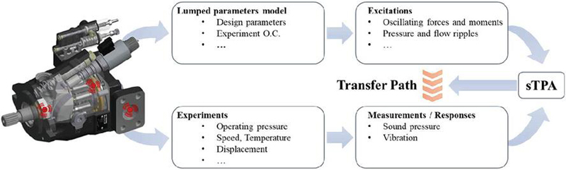
The conceptual LPM + sTPA framework is shown in the diagram in Figure 1. The pump sound and vibration measurements are carried out for multiple operation conditions, and LPM simulation is also conducted for the same operation conditions. sTPA is the processing tool for both the sound and vibration response data acquired in measurement and internal excitations data simulated using LPM. By feeding sTPA the excitation and response data for multiple operation conditions, sTPA estimates frequency response functions (FRFs) that characterize the transfer paths between excitation and response.
Figure 1 LPM+sTPA framework.
Coupling LPM with sTPA has advantages in noise/vibration mitigation of pumps. sTPA requires simultaneous data of internal excitation, and LPM provides high-fidelity data of internal excitations which is otherwise difficult to measure. With sTPA, the reductions in internal forces/moments/ripples can be quantified in terms of noise/vibration level reductions. sTPA not only fills the gap between internal excitations and consequent noise/vibration level but also provides guidelines on noise/vibration mitigation of the pump. By inspecting the FRF and path contributions, one can identify the critical transfer paths. Once the critical paths are identified, noise/vibration mitigation measures can be explored using the estimated FRFs.
The aforementioned sTPA relies on a dedicated LPM for the hydraulic circuit to provide the excitation data. When such LPM is not available, measurement-based sTPA can be conducted to analyze the relation between pump vibration and consequent noise. The air-borne noise emitted from the pump is caused by pump surface vibration. Therefore, the surface vibration can be regarded as excitation and the air-borne noise as a response. By conducting surface vibration measurement and noise measurement simultaneously, the relation between pump vibration and noise can be characterized, and the effects of pump case modifications can be then explored and evaluated.
In this paper, the development of piston unit LPM is covered in Section 2. The methodology of sTPA is introduced in Section 3. The sTPA results, including transfer path FRF, path contributions, and sensitivity analysis are shown in Section 4. The conclusions of the study are presented in Section 5.
The mathematical model for simulating axial piston pump swashplate type is described in detail in this section. The model allows for the evaluation of the unit performance under both steady-state and dynamic conditions. It has been designed and implemented to be parametric, which means that it provides the flexibility to vary the geometric parameters of a unit or a specific feature and see their effects on the performances compared to a baseline design. Figure 2 shows the cross-sectional view of an axial piston machine swashplate type with the main components considered for the model implementation labelled.
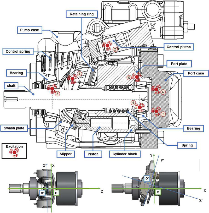
Figure 2 Axial piston pump cross-section and reference system.
Two reference systems were selected. A fixed cartesian coordinate system is considered center at the center of the instantaneous rotation of the swashplate and a mobile coordinate system is considered center on the swashplate. The eccentricity of the swashplate is considered a design parameter as well. Figure 2 shows the main point that represents a source of excitation that contributes to noise generation. Internal forces and moments have the potential to excite the pump housing, resulting in the pump vibration which results in air-borne noise. The excitation includes 1⃝ the force from the swashplate, 2⃝ the pressure ripple in the swashplate control cylinder, 3⃝ & 4⃝ the force from the shaft through the two bearings, 5⃝ the force on the port case from the cylinder block, and 6⃝ & 7⃝ the pressure ripples in the inlet and outlet port of the unit. The swashplate force and the bearing force are not considered because they are located next to the mounting interface where due to the rigid connection the housing is not free to deform. The pressure ripple in the swashplate control system is neglected because relatively low. The pressure ripple in the inlet and outlet port will result in more fluid-born noise, but limited air-borne. Therefore, the remaining excitations are the ones that affect the port case of the pump which are going to be the focus of this study.
To model the fluid dynamic behavior of the unit, a lumped parameter method has been chosen. The first step is to discretize the unit into its equivalent fluid dynamic block diagram, shown in Figure 3. Where the entire pump fluid dynamic system is represented as a set of discrete components each characterized by lumped parameters such as volume, pressure, and flow rate. For simplicity is assumed that the unit is working in pumping mode, and the flow flows from left to right.
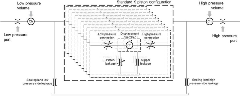
Figure 3 Axial piston pump fluid-dynamic block diagram.
To model the fluid dynamics within the axial piston machine, it is essential to analyze both its kinematic behavior and the influence of component motion on the fluid path.
An axial piston pump typically features two ports: one for suction and one for delivery. In the pumping mode, the suction port operates at low pressure while the delivery port operates at high pressure. A fixed orifice is selected to model the ports, while a fixed volume is chosen to simulate the dead volume that is present inside the port case. The structure of the pump’s rotary group includes: shaft, cylinder block, pistons, and slippers. Traditionally, swashplate-type units feature configurations with nine pistons. During a single shaft revolution, each piston performs two primary actions: suction and delivery. In the suction phase, the piston moves out from the displacement chamber, allowing fluid to enter. In the delivery phase, the piston moves into the displacement chamber, pushing the fluid out. This process is repeated every shaft revolution, with the piston communicating with the low-pressure side during suction and the high-pressure side during delivery. A variable orifice is employed to model the opening and closing between the low and high-pressure sides of the pump.
The equation representing a variable orifice is the orifice equation, which can be expressed as follows:
| (1) |
The subscript “i” in the equation generalizes its form to a vectorial representation, where the “i” element corresponds to the “i-th” piston. is the effective flow area for each piston. Its profile during a single revolution is crucial for replicating the proper behavior of the unit. The area profile depends on the design of the valve plate shown in Figure 4, which regulates the timing for connecting the displacement chamber with the low and high pressure.
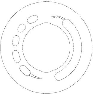
Figure 4 Valve plate.
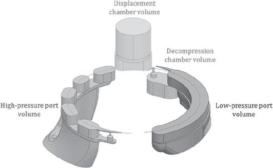
Figure 5 Fluid volume analysis.
To evaluate the area profile, the AVAS toll was used. AVAS, expanded as Automated Valve Plate Area Search, is an in-house software that solves for a minimum area of cross-section of the fluid geometry (shown in Figure 5) normal to the flow streamline for every desired step angle in a shaft revolution. This area is the smallest opening between the cylinder clock and the valve plate in the direction of flow between the displacement chamber and the high-pressure or low-pressure ports.
The pressure within the displacement chamber changes and these variations can be described by the pressure build-up equation.
| (2) |
This equation represents the instantaneous relationship that connects the pressure variation in the chamber to the sum of the flows and the volume variation It is also essential to consider the leakages from the three main lubricating interfaces. These leakages are approximated considering a laminar flow, with a constant gap height and with a linear or exponential pressure gradient. The laminar flow approximation, characterized by a low Reynold number, simplifies its complexity making it suitable for a lumped parameter approach. The model considers the piston/cylinder block interface, slipper/swashplate interface, and cylinder block/valveplate interface assuming a laminar interface with a constant parallel/concentric gap height and their expression can be found analytically [13].
This section presents a simplified study of the mechanical components of the axial piston unit. For each individual component, equilibrium equations for translation and rotation were developed, allowing the evaluation of the forces and moments exerted on a single component. The reference coordinate systems and nomenclature of the main geometric points that define the motion of the pistons and slippers are shown in Figure 2. A free-body diagram approach has been used to define the equations that describe the kinematics and dynamics of the main elements. Particular attention was focused on the port case.
The displacement chamber exerts a pressure force acting against the cylinder block. This force is then transferred to the port case via the valve plate. A thorough evaluation of the equilibrium of forces and moments is performed to determine which component may be influencing the noise emission of the hydraulic machine. The valve plate is considered to be simplified to a two-dimensional plane. Figure 6 shows how a reference system is set up in the center of the port case.
| (3) |
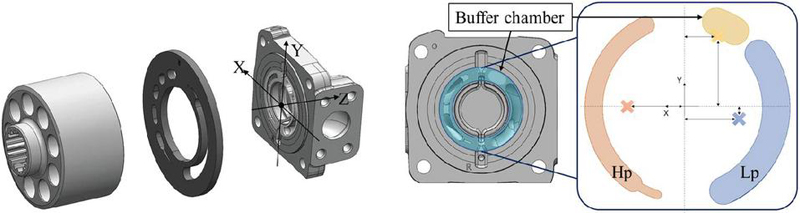
Figure 6 Port case notation.
Where represent the force applied on the port case, is the pressure force from the displacement chamber, and is the force from the valve plate. The force exerted by the valve plate is evaluated using three pressure values: low pressure, high pressure, and pressure within the inlet baffle chamber (Patent applied EP347171A1). Each of these pressures, multiplied by their corresponding area (as shown in Figure 6), produces a force opposite to the one generated by the cylinder block. The resulting force is expected to transfer to the port case. A three-dimensional computer-aided design (3D-CAD) study was used to determine the center of each region, resulting in coordinate coordinates relative to the x and y axes. A study of the moments operating on the port case was done assuming that the force generated by each area would is applied to its geometrical center.
| (4) |
Where is the moment acting on the port case around the x-axis. A similar approach has been applied to determine the moment around the y-axis .
Another excitation to consider for the sTPA is the bearing force. Due to the operating condition and working principle, each piston exerts a force on the swashplate through the slipper. Since the swashplate is inclined, a side load is generated on the piston which is then transferred to the cylinder block. The cylinder block is assumed to be rigidly connected to the shaft through a splined interface, so, the side load is then transferred on the shaft. The midpoint of the spline serves as the reference point for transmitting the force. Ultimately, the bearing needs to hold the load on the shaft. Knowing the load, transmitting point between the cylinder block and shaft, and the bearing location is then possible to evaluate the force that is exerted on the bearing.
To validate the lumped parameter model, a series of experiments were run under steady-state conditions. These tests were primarily designed to measure the pressure ripple at ’he pump’s outlet port. The experimental data were then compared to the simulated results generated by the model. The comparison aimed to evaluate the model’s accuracy. The following Figure 7 depicts the hydraulic schematic used for the experiments for model validation.
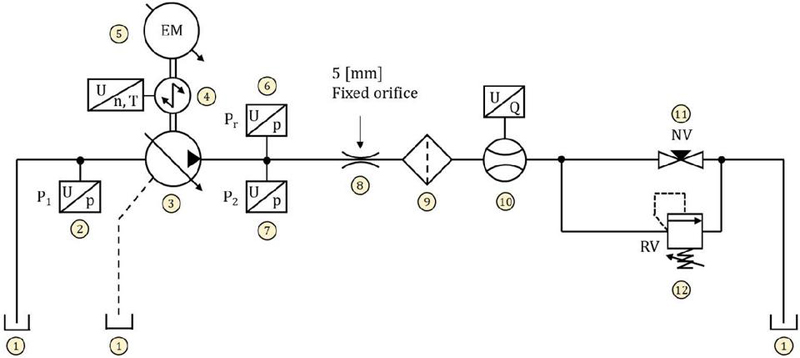
Figure 7 Hydraulic schematic.
A standard reservoir 1⃝ is connected to the unit under testing 3⃝, which is driven by an electric motor 5⃝. A torque meter 4⃝ is used to monitor speed and torque. Two pressure sensors 2⃝ and 7⃝ measure pressure differential throughout the unit, while a piezoelectric transducer 6⃝ measures pressure ripple. The pump load is regulated by a fixed orifice 8⃝, which is connected to the pressure sensors 6⃝, 7⃝ via a rigid pipe. Following the opening, a high-pressure filter 9⃝ comes before the flow meter 1⃝0. Next, a needle valve 1⃝1 is added to regulate pump load. For safety, a pressure relief valve 1⃝2 is connected in parallel.
The pump is loaded using a combination of the fixed orifice and the needle valve. The fixed orifice, along with the rigid pipe, helps assess pressure ripple under different operating conditions. Meanwhile, the needle valve provides additional back pressure, allowing for the investigation of varying pressure levels. The tests analyzed the hydraulic unit’s performance at various operating speeds and pressure levels. The unit was operated at 1000, 1500, 2000 rpm, and 2500 rpm. The pressure within the system was monitored at each speed increment, with the needle valve fully open serving as the baseline. The pressure levels obtained by adjusting the needle valve opening to reach 75, 125, and 175 bar offered insight into the unit behavior across the speed range, assisting in the validation and calibration of the lumped parameter model. A series of custom components were developed to create a comprehensive library of components that allows for a detailed simulation of the fluid dynamic model of the unit, similar work can be found in [11, 12]. This new library contains customized components modeled according to physical principles, with parametric and vectorial properties, including the parameter for the number of pistons was then integrated into the Amesim environment. To allow a smooth integration, all the components were modeled following Amesim logic for the variable flow.
To consider the loading condition, the model uses standard components already present in the Amesim library for modeling the rigid pipe and the orifice. Then, it is assumed that the pressure ripple is affected by orifice pressure drop, so a pressurized tank is used to generate the pump load. The validation of this model involves the comparison of the pressure ripple measured at the pump’s outlet port. The model does not take into account the micro motion of the components, pressure deformation, thermal deformation, and the lubricating interfaces are simplified with a constant gap height.
An FFT analysis was conducted on the measurements, revealing that 2000 rpm was the optimal configuration for validating the model due to its lower noise levels compared to other operating speeds. Additionally, the higher noise in the measurements might be attributed to the nonlinearity of the physical components present in the hydraulic circuit, which can be challenging to model using a lumped parameter approach. The following Figures 8 and 9 show the comparison of the pressure ripple measured and the pressure ripple simulated.
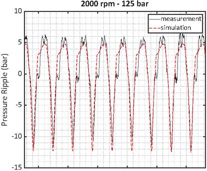
Figure 8 Sim–vs Mes – 1.
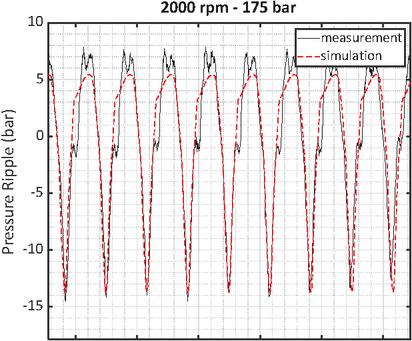
Figure 9 Sim–vs Mes – 2.
As can be noticed, the model is able to capture the pressure ripple amplitude respect different level of pressure and follow the measurement profile. The comparison on the pressure ripple amplitude led to the following evaluation of the model accuracy
| Speed [rpm] | Pressure [bar] | Mes Ripple [bar] | Sim Ripple [bar] | Error [%] |
| 2000 | 175 | 20 | 19.14 | 4.30 |
| 2000 | 125 | 16 | 17 | 6.25 |
| 2000 | 75 | 13.5 | 14.3 | 5.93 |
The results show that the model can simulate the pressure ripple with an average error of 5.5% with respect to the measurement results.
Transfer path analysis (TPA) is a technique used to break down noise or vibration into its key contributors. The noise/vibration contributors are characterized using frequency response functions from excitations to the acoustic/vibration responses at target locations.
The three major components in the TPA calculation are:
• Excitations: The spectrum of forces/moments source that causes noise and vibration.
• Responses: The noise/vibration acquired at target locations.
• Transfer Paths: The mathematical relation that characterizes how noise and vibration are transferred from source excitation to the responses.
Figure 10 shows the relation of excitations, responses, and the transfer paths in between for a mechanical system with 3 excitations, 2 responses, and 6 transfer paths. In general, if there are excitations and responses, the number of transfer paths is -by-. The task of TPA is to determine the frequency response functions (transfer functions) for each transfer path mathematically.
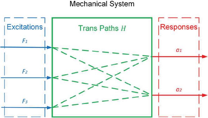
Figure 10 Excitations, responses, and transfer paths in TPA.
TPA has been a widely used engineering tool for the analysis of mechanical vibration transmissions for a variety of industrial products, and the methodologies of TPA have kept developing over time. Van der Seijs et al. provide a compressive review of the landscape of TPA methods [14]. In the conventional practice of TPA, the excitations are isolated and applied to the mechanical system individually. In the example shown in Figure 10, if excitation is isolated and applied, then the frequency response function from to responses and can be simply calculated as and .
However, for axial piston pumps, it is difficult to isolate excitations and apply them individually. For example, in an operating hydraulic pump, the oscillatory fluid pressure ripples cause noise and vibration, yet it is difficult to investigate the fluid pressure related transfer path alone, without introducing other simultaneous excitations such as the bearing force due to pressure imbalance across cylinders. For this reason, a sub-category of TPA methodology, simultaneous TPA (sTPA, also referred to as operational TPA), is thus more suitable for the estimation of transfer path FRFs for such mechanical systems. sTPA has gained popularity in multiple engineering areas as an NVH analysis tool [15–18], due to its ease of setup the measurement. Instead of isolating and applying excitations individually, in the practice of sTPA, multiple independent combinations of operational excitations are created by altering the operation conditions of the mechanical system. Assume the system is tested under operation conditions, the mathematical relation of excitations, responses, and transfer paths can be cast in a matrix form:
| (5) | ||
| (6) |
In which represents the i-th response at the k-th operation condition, represents the j-th excitation at the k-th operation condition, and is the ratio of to . For piston pumps, can be responses that characterize noise/vibration of the unit, such as sound pressure or pump housing vibration acceleration. can be variables such as pressure/flow ripples or bearing forces, which characterize noise/vibration inducing mechanisms of the pump. In sTPA, is a frequency-dependent matrix containing responses such as sound acceleration, velocity or sound pressure, acquired by sound/vibration test. is a frequency dependent matrix acquired from LPM simulation that contains the source magnitude and phase. The independence of excitations can be verified by stacking matrix of different frequencies row-wise and calculating the rank of the stacked matrix. A rank equal to indicates mutually independent operational excitations.
Given and , the i-th row of be estimated as:
| (7) |
in which . It should be noted that for Equation (7) to be valid, the number of operation condition needs to be greater than or equal to the number of excitations .
Equation (7) provides a least-square estimate of , such that norm is minimized, in which . Since the number of operations conditions is larger than the number of excitations , overfitting of the transfer path FRF can occur. In order to avoid such overfitting of FRF, a regularized least-square formulation is used to replace Equation (7). The regularized least square formulation minimizes , in which is the parameter of regularization. is chosen such that generalized cross validation (GCV) function is minimized.
| (8) |
It should be noted that different rows of matrix has different units. Consequently, when the least-square formulation is evaluated, the unit system applies different weights to rows of . To eliminate the effect of unit system of choice, a normalization process is applied to matrix as
| (9) |
which are average values for j-th excitation over all operation conditions. Such normalization process makes dimensionless.
The method of sTPA is validated against analytical solutions of baffled pistons. The sound field of a baffled piston can be written as
| (10) |
Therefore, the analytical FRF between piston volumetric displacement and radiated sound can be simply cast as . If pistons are operating simultaneously with volumetric displacement respectively, the resulting sound field can be calculated at field points using Equation (10). Providing different operation conditions of pistons (In this case, operation conditions are represented by independent combos of ), the problem can be formulated as in Equation (5), and the FRF can be found by sTPA. The results demonstrate total agreement as shown in Figure 11.
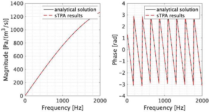
Figure 11 FRF of baffled pistons.
A comprehensive investigation of a 45cc pump was conducted where data for sTPA is obtained by two distinct testing procedures. In test 1, the relation between pump internal excitations and its noise/vibration was explored by using LPM simulation data as excitations and using pump noise and vibration measurement data as responses. In test 2, an extended sound and vibration measurement is conducted, the measured vibration and noise data were utilized as the sTPA excitations and responses respectively, in order to investigate the relation between pump vibration and its air borne noise emission. The differences of the two tests are shown in Figure 12.
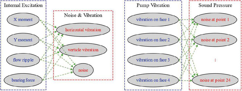
Figure 12 sTPA diagrams. Left: Test 1 – transfer paths from internal excitation to pump noise and vibration; Right: Test 2 – transfer paths from pump vibration to pump noise.
In the first test, a 45cc pump was tested under 18 different operation conditions. The pump was controlled to run at a constant speed with two different configurations: (1) Configuration A, where a fixed orifice of 5 mm is located next to the outlet port of the pump, followed by a 3 m hose, and (2) Configuration B, where the fixed orifice and the hose positions are switched. For both configurations, tests were run for three pressure levels 50, 175, and 300 bar, and three different levels of swashplate angles were tested for each pressure level: 0%, 50% and 100%. It is noted that the pump speed is kept constant in the case study, however, the method of sTPA is, in general, valid for any pump speeds. Accelerations at two locations and sound pressure at one location are acquired. The placements of the sensors are shown in Figure 13. The two accelerometers measure horizontal (Z-axis) acceleration and vertical (Y-axis) acceleration respectively. Sound pressure is measured 1 meter away along Z direction from the pump. In the second test, noise and surface vibration was measured with the pump mounted in a semi-anechoic chamber and pump speed fixed at 2000 rpm. By varying pressure (63 bar to 234 bar) and swashplate angle (50% and 100%), a total of 20 operation conditions were tested. Surface vibration of the pump is measured at four different locations simultaneously, as shown in Figure 13. Microphones are mounted on a scanning arm and the noise signal of the pump is acquired from 24 locations evenly distributed over a hemisphere with 1 meter radius that encloses the pump. Tachometer measurements are utilized to synchronize noise measurements at different scanning positions. Figure 14 shows the spectra of noise and vibration of one typical operation condition. The spectral peaks coincide with the piston frequency (300 Hz) and its harmonics, indicating that the major noise/vibration inducing mechanism is associated with the periodic piston motions.
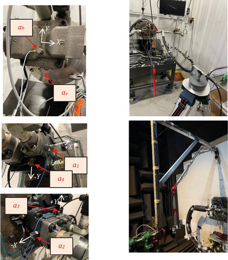
Figure 13 Sensor placement. Top-Left: Accelerometers (Test 1); Top-Right: Microphone (Test 1); Bottom-Left: Accelerometers (Test 2); Bottom-Right: Microphone scanning arm (Test 2).
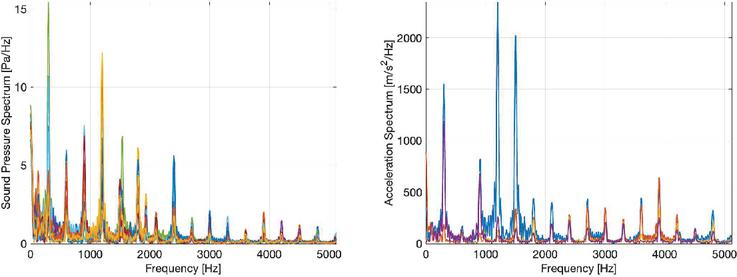
Figure 14 Noise and vibration spectra for operation condition: 183 bar, 50% swashplate angle. Left: Noise spectra from 24 measurement locations. Right: Vibration spectra from 4 measurement locations.
LPM simulations were conducted for all 18 different operation conditions. The excitations taking into consideration in the present study are bearing force component in y-direction (see Figure 6) , sealing land moments and and flow ripple . An example of excitation simulation results is shown in Figure 15.
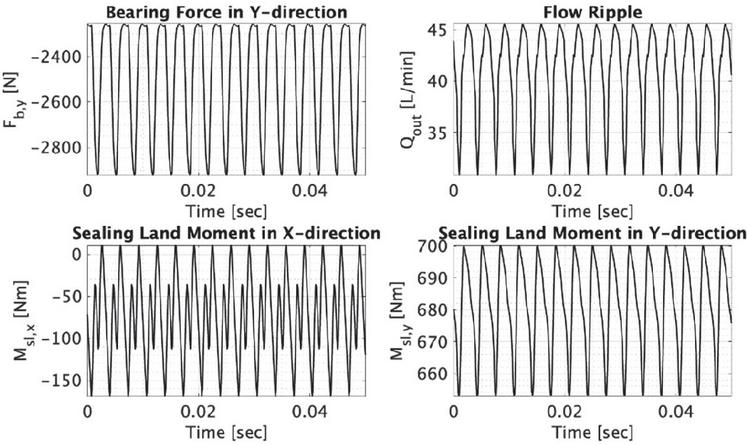
Figure 15 LPM simulation results of excitations. Operation condition: 300 bar, 50% swashplate angle, configuration B.
Due to the cyclic nature of pump operation, Fourier coefficients of both simulation and experiment data were calculated. Because the measurement and simulation do not have the same starting time, phase differences arise when comparing measurement and simulation data. The phase difference between simulated excitations and sound and vibration measurement results were estimated and compensated by introducing appropriate time delay to the results.
The Frequency Response Functions (FRF’s) in Figure 16 shows how effectively noise/vibration transfer paths of the pump unit amplifies the input excitations (internal excitations or surface vibration) into noise and/or vibration at different frequencies. The magnitude amplification factors are displayed in decibels using a color scale. Each colored block in the figure represents an amplification factor which physically represents how much noise or vibration would be produced by a input force with unit strength at that frequency.
While the FRF shows stronger amplification (higher values) at higher frequencies, the actual noise and vibration levels depend on both the FRF and the strength of input forces at each frequency. In test 1, despite having moderate FRF values at 302 Hz, this frequency dominates the overall noise and vibration output because it coincides with the main piston movement frequency, at which the excitation is the strongest.
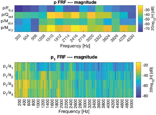
Figure 16 Frequency response functions.Top: Test 1 FRF between excitations simulated in LPM (, , and ) and noise ; Bottom: Test 2 FRF between pump vibration () and noise .
In order to analyze the root-cause of noise and vibration of piston pumps, path contributions are calculated using FRF estimated using sTPA. For the k-th operation condition, path contribution of the j-th excitation to the i-th response is , and therefore a path contribution demonstrate the combined effect of both the strength of excitations and FRF amplifications. The synthesized response is the summation of all the path contributions, that is, . Path contributions and synthesized responses are complex and can be drawn on complex planes. Figure 17 shows the path contribution of an operation at piston frequency as an example. Each solid arrow in the figure represents a contribution from an excitation to either a vibrational or acoustical response. The solid arrows connect head-to-tail to form the synthesized response. The figure visualizes the significance of individual transfer paths as well as the cancellation/enhancement effects among various paths. For instance, the individual contributions of and to horizontal vibration both have large magnitude, yet they destructively interfere against each other because of 130 degrees phase difference. The contributions to , on the other hand, are in phase with each other and contribute evenly to the response. The measurement value is also shown in Figure 17 for reference, and the difference between measurement and the sTPA synthesized response is due to the frequency response functions for being overdetermined. Specifically, because the number of constraints is equal to the number of operation conditions and is greater than the number of excitations, the FRF calculated in sTPA is an approximation such that the regularized least square formulation in Section 3 is minimized. Figure 18 shows a time domain comparison between the synthesized response and the measured response to visualize the error between sTPA synthesized response and the actual response.
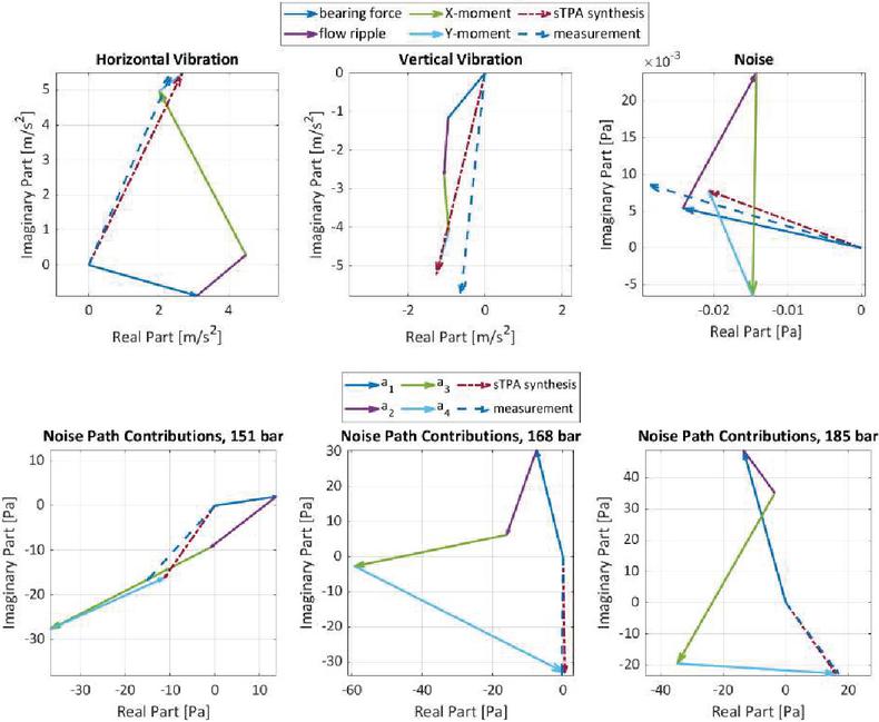
Figure 17 Path contributions. Top: Test 1, operation condition: 300 bar, 50% swashplate angle, configuration B. Bottom: Test 2, operation condition: 151, 168, 185 bar, 100% swashplate angle.
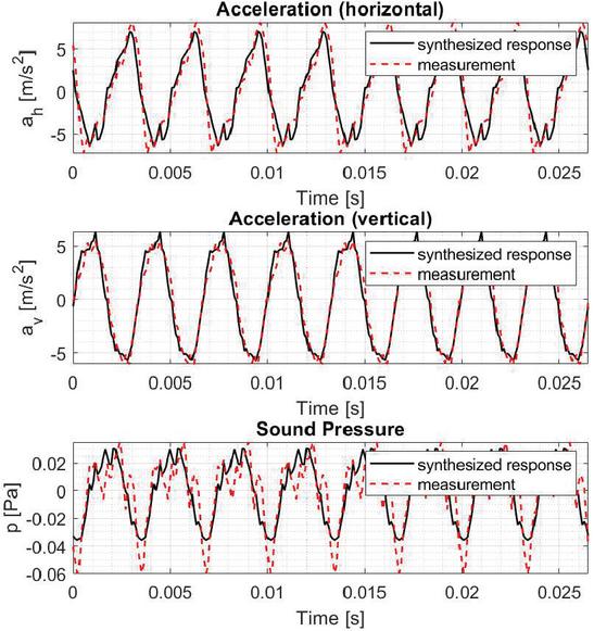
Figure 18 Time domain comparison between synthesized response and measurement.
Sensitivity analysis can be conducted based on the information of sTPA predicted path contributions. In this study, the sensitivity of noise and vibration responses to excitation magnitudes are analyzed. The overall sound pressure or acceleration level is used as the metric of noise/vibration performance of the pump. The overall level of the i-th response is calculated as
| (11) |
is the reference value for the i-th response and its value is 10 m/s and 20 Pa for acceleration and sound pressure respectively.
The sensitivities of the three responses (, and ) to the magnitude of the four excitations (, , and ) are shown in Figure 19. The magnitude of each excitation is set to independently vary over a 20% range (the change of one excitation does not affect other excitations), and the overall levels of synthesized responses are evaluated. The red dashed lines in the figures indicate the reference point. As shown in the figure, all the curves are monotonically increasing, which implies the positive correlation between force/moment/ripple excitations and noise/vibration responses. The figure also indicates potentials of noise and vibration control. For example, the overall sound pressure level can be decreased by 0.70 dB (from 64.79 dB to 64.09 dB) if the oscillations in X-moment decrease by 20%, overall horizontal acceleration decreases by 1.73 dB (from 115.81 dB to 114.08 dB) if X-moment oscillation decreases by 20%. Sensitivity analysis implies that pump noise and vibration exhibit maximum sensitivity to the X-moment excitation, and design modification that reduces X-moment oscillation would benefit pump NVH performance the most.
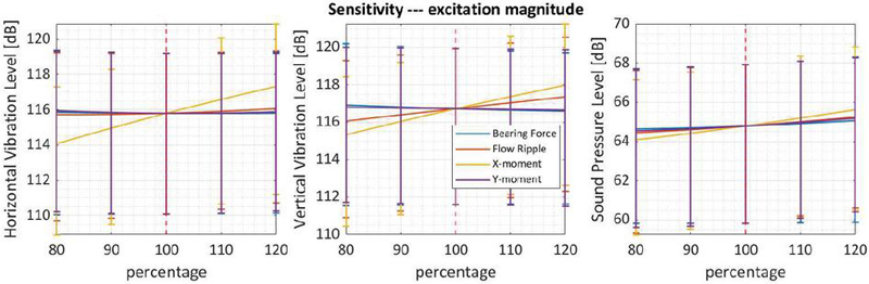
Figure 19 Sensitivity of noise and vibration response to excitation magnitudes.
A further comment on the generality of the sensitivity analysis needs to be emphasized. In such analysis, it is assumed that the transfer paths are not altered as parameters vary. For example, the graph shown in Figure 19 can be interpreted as predictions of pump noise and vibration, only if the magnitude of excitations can increase/decrease without changing the characteristics of transfer paths. On the other hand, if the change of parameter is associated with change in pump design, the parameter sensitives are not predictive, and sTPA can only be seen as an additional analysis to close the gap between LPM simulation and pump NVH.
The sensitivities of the spatially averaged sound pressure level to magnitude of the four vibration accelerations are shown in Figure 20. Contrary to Figure 19, in the sensitivity analysis of excitation magnitude, the sensitivity curves are not monotonically increasing, which implies that there are optimal magnitudes for each vibration acceleration. For example, optimal sound pressure level can be reached if increases by 7%, whereas sound pressure level can be decreased by 0.182 dB and 0.072 dB if and decreases by 8% and 6% respectively. Since the vibration of different pump locations exhibits distinct relation to noise emission, it can be predicted that the effect of vibration damping surface treatment is sensitive to the location where surface damping is applied.
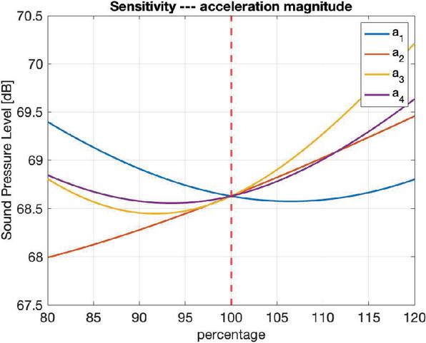
Figure 20 Sensitivity of noise and vibration response to excitation magnitudes.
A novel LPM+sTPA framework is developed for the root-cause analysis of pump noise and vibration. The uniqueness of this method is to combine simulations for excitations and measured responses, which allows TPA for operating machines where excitations cannot be physically measured. The LPM+sTPA framework is applied to the analysis of hydraulic pump noise and vibration to bridge the gap between the operation of the pump and its noise/vibration performance. The results of sTPA can reveal the root-cause of noise and vibration problems of axial piston pumps. Path contributions estimated in sTPA demonstrate how different sources of noise and vibration add up to the overall noise and vibration effect of the pump and highlight the most significant noise/vibration contributor. Based on the sensitivity analysis of sTPA, the potential pump noise/vibration control measures can be evaluated in terms of noise/vibration level decrement.
The authors identify X-moment excitation as a key contributor to noise in a case study; therefore, future research could focus on designs aimed at reducing X-moment using the lumped parameter model could be used for preliminary investigations of new design solutions. The LPM+sTPA method could be leveraged to identify noise sources in other hydrostatic machines such as piston unit bent axis type. The case study demonstrates the advantage of the LPM+sTPA methodology: it provides insights into targeted design improvements while establishing a versatile framework applicable across various hydrostatic machine configurations. It enables engineers to precisely identify and address noise sources without doing challenging physical measurement of internal excitations. Rather than trial-and-error approaches, pump design optimization focusing on noise/vibration reduction is possible with the aid of LPM+sTPA method.
[1] Schleihs, C. (2017). Acoustic Design of Hydraulic Axial Piston Swashplate Machines. Reihe Fluidtechnik, 89. RWTH Aachen University.
[2] Helgestad, B. O., Foster, K. and Bannister, F. K. (1974). Pressure transients in an axial piston hydraulic pump. Proceedings of Institution of Mechanical Engineers. 188(1):189–199.
[3] Yamauchi, K. and Yamamoto, T. (1976). Noises generated by hydraulic pumps and their control method. Mitsubishi technical review, 13(1).
[4] Kim, T. and Ivantysynova, M. (2017). Active Vibration Control of Swash Plate-Type Axial Piston Machines with Two-Weight Notch Least Mean Square/Filtered-x Least Mean Square (LMS/FxLMS) Filters. Energies. 10(5):645.
[5] Harrison, A. M. and Edge, K. A. (2000). Reduction of axial piston pump pressure ripple. Proceedings of Institution of Mechanical Engineers, Part I: Journal of Systems and Control Engineering. 214(1):53–64.
[6] Ortwig, H. (2005). Experimental and analytical vibration analysis in fluid power systems. International Journal of Solids and Structures. 42:5821–5830.
[7] Rebel, J. (1977). Active liquid noise-suppressions in oil hydraulics. VDI-Z. 119:937–943.
[8] Tanabe, Y., Watanabe, M., Aoki, T., Ikeda, K. and Takeshita, S. (2008). Transfer Path Analysis to Hydraulic Excavator for Reducing Cabin Noise Caused by Hydraulic Pulsation. INTER-NOISE and NOISE-CON Congress and Conference Proceedings, InterNoise08. Shanghai, China, pp. 4214–4220(7).
[9] Opperwall, T. and Vacca, A. (2015) A Transfer Path Approach for Experimentally Determining the Noise Impact of Hydraulic Components. SAE Technical Paper. 2015-01-2854.
[10] Pan, Y., Li, Y., Huang, M., Liao, Y. and Liang, D. (2018). Noise source identification and transmission path optimisation for noise reduction of an axial piston pump. Applied Acoustics. 130 (2018) 283–2.
[11] Manco, S., Nervegna, N., Lettini, A. and Gilardino, L. (1999). An experience in simulation: the case of a variable displacement axial piston pump. JFPS International Symposium on Fluid Power.
[12] Manco, S., Nervegna, N., Lettini, A. and Gilardino, L. (2002). Advances in the simulation of axial piston pumps. JFPS International Symposium on Fluid Power.
[13] Ivantysyn, J. and Ivantysynova, M. (2001). Hydrostatic pumps and motors.
[14] Van der Seijs, M., de Klerk, D. and Rixen, D. (2015). General framework for transfer path analysis: History, theory and classification of techniques. Mechanical Systems and Signal Processing. 68–69: 217–244.
[15] de Klerk, D. and Ossipov, A. (2010). Operational transfer path analysis. Mechanical Systems and Signal Processing. 24: 1950–1962.
[16] de Sitter, G., Devriendt, C., Guillaume, P. and Pruyt, E. (2010). Operational transfer path analysis. Mechanical Systems and Signal Processing. 24: 416–431.
[17] Roozen, N. B. and Leclère, Q. (2013). On the use of artificial excitation in operational transfer path analysis. Applied Acoustics. 74: 1167–1174.
[18] Sievi, A., Martner, O. and Lutzenberger, S. (2013). Noise Reduction of Trains Using the Operational Transfer Path Analysis – Demonstration of the Method and Evaluation by Case Study. In: Maeda, T., et al. Noise and Vibration Mitigation for Rail Transportation Systems. Notes on Numerical Fluid Mechanics and Multidisciplinary Design, vol. 118. Springer, Tokyo.

Dazhuang He is a Ph.D. student in Mechanical Engineering at Purdue University, where he conducts research on multiphysical noise and vibration analysis of positive displacement fluid machinery. His work integrates thermodynamics, fluid dynamics, and vibroacoustic modeling to develop predictive simulation frameworks. His current research focuses on vibroacoustic analysis through advanced numerical methods.

Antonio Masia is a Ph.D. candidate in the Department of Agricultural and Biological Engineering at Purdue University, specializing in fluid power systems and tribology. His research focuses on the design and experimental analysis of hydrostatic machines, with an emphasis on tribological performance and surface engineering.

Yangfan Liu is an Assistant Professor of Mechanical Engineering at Purdue University. His research focuses on acoustic source modeling, active noise control, room acoustics simulation, noise control treatments, and the human perception of noise. Dr. Liu is affiliated with the Ray W. Herrick Laboratories at Purdue University.

Lizhi Shang is an Assistant Professor of Agricultural and Biological Engineering and Mechanical Engineering at Purdue University. His research focuses on designing and modeling hydrostatic pumps and motors, hydrodynamic pumps and turbines, and fluid power systems. He also conducts advanced computational and experimental tribological analysis to enhance energy efficiency, reliability, and controllability of fluid power systems. Dr. Shang is affiliated with the Maha Fluid Power Research.

Daniel Dyminski is a Principal Engineer at Parker Hannifin, specializing in fluid power systems. He has a background in mechanical engineering and has been involved in research and development within the field. His work focuses on the design and analysis of hydraulic components and systems, contributing to advancements in fluid power technology.
International Journal of Fluid Power, Vol. 26_2, 289–318.
doi: 10.13052/ijfp1439-9776.2627
© 2025 River Publishers